Abstract
The emission of greenhouse gases from public transportation has aroused extensive public attention in recent years. Electric buses have the advantage of zero emission, which could prevent the further deterioration of environmental problems. Since 2018, the number of electric buses has exceeded that of traditional buses. Thus, it is an inevitable trend for the sustainable development of the automobile industry to replace traditional fuel buses, and developing electric buses is an important measure to relieve traffic congestion. Furthermore, the bus scheduling has a significant impact on passenger travel times and operating costs. It is common that passenger demand at different stops is uneven in a public transportation system. Since applying all-stop scheduling only cannot match the passenger demand of some stops with bus resources, this paper proposes an integrated all-stop and short-turning service for electric buses, reducing the influence of uneven ridership on load factor to enhance transit attractiveness. Simultaneously, considering the time-of-use pricing strategy used by the power sector, the combinational charging strategy of daytime and overnight is proposed to reduce electricity costs. Finally, the branch-and-price algorithm is adopted to solve this problem. Compared with all-stop scheduling, the results demonstrate a reduction of 13.5% in total time cost under the combinational scheduling.
1. Introduction
1.1. Background
Electric buses (EBs) with the characteristics of low noise, low pollution, and high driving stability can effectively alleviate a series of problems, such as energy shortage, environmental pollution, and traffic congestion. Therefore, urban public transportation is more environment-friendly with the popularization of the electric bus. Extensive literature is available about the EBs, including vehicle scheduling problem (VSP) [1], integrated timetabling [2], and charging planning [3].
In the real world, the passenger flow is unevenly distributed along the route. It is common that the arrival number of passengers at several stops accounts for a large proportion of the total passenger flow, while that at other stops only accounts for a small proportion. Under this circumstance, all-stop scheduling, in which the bus serves all stops on the line, causes the load factors of vehicles to vary greatly at different stops, while in the integrated all-stop and short-turning service, the bus serves continuous stops with high passenger flow on a segment of the line, which can reasonably allocate bus resources under uneven demand distributions. Moreover, more vehicles are provided to the overcrowding stops to improve the comfort of passengers and the public transportation attraction.
Electric buses have charging demand in the process of operation, which are different from fuel buses. Charging at different times will affect the formulation of vehicle scheduling schemes as well as charging costs. Therefore, a reasonable charging strategy can improve vehicle-scheduling schemes and reduce the electricity costs of public transportation.
It is greatly necessary to study a combinational scheduling strategy and corresponding charging strategy of electric buses for the purpose of matching the transport capacity of electric buses with the passenger flow and improving the efficiency of vehicle operation. Before our studies, the scope of the study focuses on frequent services in urbanized areas because in such a condition, there is a large possibility that an uneven distribution of passenger flow occurs and most passenger flow is concentrated in some consecutive stops. It is necessary to add short-turning buses on the line. In addition, we assume that the overtaking behavior is not allowed during the operation.
1.2. Related Works
Timetabling design and vehicle scheduling problems have been extensively studied mainly from four aspects [4,5,6,7,8], which are all-stop scheduling with conventional buses, all-stop scheduling with EBs, conventional buses under multi-mode operation strategies, and the charging strategies of EBs [9,10,11,12,13,14].
Typically, the scheduling of conventional buses with the all-stop strategy contains timetabling design and a vehicle scheduling scheme. Carosi et al. (2019) considered vehicle scheduling and timetabling and used the weighted objective function to establish the bi-objective nature of the integrated TT-VS (time tabling-vehicle scheduling) problem. Additionally, this paper proposed a mixed integer linear programming multicommodity-flow type model to optimally balance the service provider cost, which is the objective of vehicle scheduling and the user satisfaction, which itself is the objective of timetabling [15]. Shang et al. (2019) presented a timetabling method in view of passenger satisfaction for the purpose of optimizing the bus frequency and headway. The timetabling is optimized by considering a balance between passenger satisfaction and the bus transit efficiency, explicitly considering the load factor [16]. Zhang et al. (2020) proposed a new model to design a timetabling adjusted to the dynamic passenger flow considering both passenger comfort and bus company objective on resource utilization. This study can adjust headways to adopt to the variations in the passenger flow [17]. Zhang et al. (2020) presented a bi-objective optimization model for a feeder bus line to minimize operating costs and passengers waiting times with consideration of three different types of buses and proposed a decomposition heuristic algorithm to address the multiple vehicle-types scheduling problem [18]. Peña et al. (2019) presented a timetable optimization method based on a multi-objective cellular genetic algorithm, with the aim of optimizing a quality of service and transport operating costs under multiple vehicle-type problems [19]. Gkiotsalitis and Alesiani (2019) developed a robust timetable by applying a bus movement mathematical model that combines the uncertainty of travel times and passenger demand to minimize the possible loss at worst-case scenarios under considering the travel times and passenger demand uncertainty [20]. Wang et al. (2020) developed a dynamic bus scheduling problem that is able to quickly produce a scheduling scheme to solve the impact of a great number of bus schedules because of the large-scale traffic congestion. In addition, this study verified the effectiveness of multi-objective optimization approach [21].
The timetabling design and vehicle scheduling with EBs of all-stop scheduling take recharging and driving range into consideration [22,23,24,25]. Teng et al. (2019) introduced a multi-objective particle swarm optimization algorithm to optimize the single-line bus timetabling and VSP that smoothes the headway and minimizes the number of vehicles and charging cost [26]. Ke et al. (2020) optimized the battery recharging scheduling at different times during the timeframe, in an effort to minimize the single-day total cost of the public transport system [27]. In addition, this study took solar and wind power generation and different feeder loads of the main transformer into consideration, integrating demand response and the resale of battery electricity to the power company. Tang et al. (2020) developed static and dynamic scheduling models to minimize the sum of operational costs in the period and the costs expectation after the period. In order to address the adverse effects caused by trip time stochasticity, the static model introduces a buffer-distance strategy, utilizing a branch-and-price algorithm to solve the problem [28]. Alwesabi et al. (2020) developed a scheduling model for the purpose of minimizing total cost, which is the optimal number of EBs, by considering the number of the dynamic wireless charging and battery size restrictions [29]. Häll et al. (2019) optimized changes of the timetabling and vehicle scheduling taking into account the feature of electric buses and different charging techniques, such as overnight charging, continuous charging, and quick charging to minimize the number of buses used as well as the deadheading distance [30]. Rinaldi et al. (2018) presented a mixed-integer linear program formulation to decide the sequence of electric and hybrid buses departing from a multi-line bus terminal, with the constraints of service factor and charging factor [31].
The combinational scheduling with traditional buses mainly includes multimode scheduling strategies, such as integrated strategies of all-stop and short-turning strategies, combinatorial scheduling of all-stop and skip-stop tactics [32,33,34,35]. Gkiotsalitis et al. (2019) proposed a rule-based method which is short-turning and interlining lines, into the frequency and resource allocation problem to reduce passenger waiting times at stops and operational costs. As a result of the fractional, nonlinear objective function, this problem deals with exterior point penalties and a genetic algorithm meta-heuristic [36]. Cao and Ceder (2019) illustrated a new approach to establish the optimized public transport timetable incorporated with vehicle scheduling, including using the skip-stop tactic based on real-time passenger demand, in order to decrease fleet size, which represents operational costs, and reduce travel times, which demonstrates the costs to passengers [37]. Chen et al. (2018) developed a continuum approximation modeling which is integrating the local route service and the short-turning strategy to minimize the generalize costs considering passengers and transit operators [38]. Zhang et al. designed an integrated limited-stop and short-turning services for the purpose of optimizing frequencies of buses to minimize the total cost of a transit system, including user costs and operator costs [39]. Tirachini et al. (2011) presented a model of a short-turning strategy to set the optimal values of frequencies, capacity of vehicles, and the position of the short-turning limit stations to reduce the costs of the operator as well as the waiting and in-vehicle times that users spend while traveling [40]. Compared with a normal operation scheme, most demands are satisfied by this strategy.
Considering the limitation of the battery capacity, buses need to be charged for a long time in the daytime to meet the operation demand of the entire day. Thus, the charging strategy will influence vehicle scheduling to a large extent. In recent years, many papers have focused on the charging of electric buses, e.g., the charging strategy of electric buses [41,42,43,44,45], the choice of charging and route [46], charging station location planning [47,48], operating cost [49,50,51], etc. Given the charging demand of electric bus and drivers’ range anxiety, Xu et al. (2020) developed a compact mixed-integer nonlinear programming model in order to determine the optimal locations of EV charging stations with the limitation of budget. Furthermore, this paper developed an efficient outer-approximation method to obtain the ε-optimal solution to the model, and a real-life Texas highway network was utilized to verify the effectiveness of the proposed models and solution method [52]. Qin et al. (2016) utilized the data of demand charges of a fleet of electric buses in Tallahassee, Florida to simulate daily charging patterns in order to minimize demand charges [53]. He et al. (2020) established a network modeling framework to address the problems of limiting the driving range and consuming charging for electric bus systems and minimizing the total charging costs of an electric bus system to optimize the charging scheduling [54]. Wang et al. (2018) developed a real-time charging scheduling based on the Markov decision process to optimize the e-bus fleet by minimizing the overall charging costs of the e-bus fleet and maximizing fares collected for serving passengers taking account of the time-variant electricity pricing [55].
1.3. Contributions
Based on the previous studies, most of them are all-stop scheduling and multi-mode operation strategies with conventional buses. As electric buses are developing, works on electric bus scheduling are extending. However, no study has considered the uneven distribution of passenger demand when developing the scheduling method for electric buses. The adoption of short-turning strategy not only affects dispatching headways and fleet size but also the energy consumption and charging plans. In such condition, the study will be different from the scheduling of conventional fuel buses.
The main purpose of this study is to optimize the vehicle scheduling plan, the locations of starting and terminal stations for short-turning line and charging strategy simultaneously, for the bus route with all-stop strategy and shorting-turning strategy.
(1) Under the background of rapid development of electric buses, we propose the combinational scheduling strategy of all-stop and short-turning in order to match the bus transport capability with passenger demands. Some stops adopt short-turning strategies to share passenger flow and avoid increasing the operating cost.
(2) Given that the time-of-use (TOU) pricing strategy adopted by the power sector, we present the combinational charging strategy of daytime and overnight to reduce electricity costs. Specifically, charging during the semi-peak prices of daytime and overnight with the off-peak prices aims to slow down the advancement of the electricity consumption and minimize the electricity cost.
(3) In this paper, an integer nonlinear programming problem is established, which is transformed into an integer linear programming problem by traversing the departure interval. Then, the branch-and-pricing algorithm is used to solve the problem.
2. Methods
2.1. Scheduling Strategy of EBs
- (1)
- The combinational scheduling strategies
Before describing the strategy, we first illustrate the terms of the all-stop and short-turning strategy. In our study, the all-stop strategy is that the bus serves all stops on the line, arriving at the terminal station from the starting station. The short-turning strategy is an auxiliary vehicle scheduling that the bus serves continuous stops with high passenger flow on a segment of the line.
- (2)
- Charging strategy
The charging strategy will affect the electricity costs greatly, consisting of two primary components: the total electricity consumption and the electricity price. On the one hand, the total electricity consumption is influenced by the SOC, that is the state of charge of battery, at the departure time of each trip, and the higher the SOC value of a bus at the starting station, the lower the power consumption of the trip. On the other hand, most areas of China implement the time-of-use pricing policy, which means the electricity price is higher in the daytime electricity peak period and lower at night. Charging in the daytime keeps the SOC of each trip at a higher level and reduces the electricity consumption during all-day operation, but the electricity price is higher. Although the electricity price at night is lower, the SOC of each trip will continue to decline, which increases the total electricity consumption in the operation process.
Therefore, taking the electricity price as the evaluation index, we determine the optimal strategy for charging in the daytime and charging at night.
- (3)
- Optimization objectives and variables
The scheduling strategy is not only bound up with the interests of passengers but also those of bus companies. In this regard, we conduct a comprehensive consideration of three factors: passenger travel time costs, electricity costs, and the number of vehicles; since passenger travel time costs and electricity costs are calculated in days, the number of vehicles is converted into vehicle daily values by the total depreciation costs. Finally, the weighted sum of these three parts is taken as the optimization objective to establish the optimization model.
The overlapping segment is defined as the same operation range of all-stop and short-turning services. The optimization variables of the model are (1) the location of the starting and ending stations in the overlapping segment; (2) the departure intervals of buses in each period; (3) the scheduling and charging strategy of each bus; and (4) the number of all-stop and short-turning buses.
2.2. Description of the Bus Route
There are K all-stop buses and Z short-turning buses on the route. A and B represent all-stop and short-turning scheduling, respectively. denotes the running direction. A bus runs toward the up direction (from stop 1 to N) when and it runs toward the down direction (from stop N + 1 to 2N) when . The service ranges of all-stop buses and short-turning buses are the whole line and a segment of the line, respectively. We assume that charging locations are set at the starting stations of each running direction, such as stop 1, N + 1, , and .
The all-stop bus is only recharged at stop 1, N + 1, and the short-turning bus is only recharged at stop , . It is also assumed that the number of charging locations is sufficient and the SOC of all vehicles is the same at the beginning of the whole day operation.
Based on an imbalanced distribution of passenger demand over time, the operation process is separated into M time intervals, and the non-operating period at night is set as the M + 1. and are the beginning and end of the m-th period, respectively. is the duration of the m-th period.
The total number of trips for all-stop buses in period m and direction u is , which is denoted by Equation (1).
The total number of trips for short-turning buses in period m and direction u is , as denoted by Equation (2).
and represent respectively the departure intervals of all-stop buses and short-turning buses in the m-th period, min.
Equation (2) is the departure time from the start station of trip i in the direction u, , while o represents departing from the starting station for the bus.
where is the corresponding trip number of trip i in the m-th period, , i.e., and refer to the same trip. This trip is the trip in the whole day’s trips, while the trip in the trips of period m.
The departure time from the start station of trip j in the direction u, , is represented in Equation (3).
2.3. Description of EBs Operation
Waiting passengers are split into two types based on different origin–destination (OD). We set passengers whose origin and destination are in the overlapping segment as Type 1. Furthermore, they could take both all-stop buses and short-turning buses for traveling. Otherwise, passengers belong to Type 2, and they could only take all-stop buses. Thus, the passenger flow of all-stop buses and short-turning buses will affect each other.
We define two sets and . indicates the set of trips for all-stop buses in the operating direction u, where is the sum of trips for all-stop buses, . Similarly, is the set of trips for all-stop buses and short-turning buses in the overlapping segment, where , , which illustrates the total number of trips, where is the sum of trips for short-turning buses.
The arrival time at stop n is related to the dwell times of the previous n − 1 stops, depending on the number of boarding and alighting passengers at the previous n − 1 stops and the travel times from stop 1 to stop n − 1; meanwhile, the inter-stop travel time is determined by the bus travel speed and distance between adjacent stops.
Equation (4) represents the dwell time at stop n for trip q belonging to , which is determined by the opening and closing times of bus doors and the boarding and alighting times of passengers.
where and denote respectively the opening and closing times of bus doors, s; and denote respectively the boarding time and alighting time per passenger, s/pax; and represent respectively the number of boarding and alighting passengers of trip q at the stop n, pax.
The actual number of boarding passengers at stop n is the minimum value between the number of waiting passengers and the residual capacity in trip q at stop n.
where represents the number of waiting passengers for trip q at stop n, pax; denotes the bus capacity, pax; denotes the number of in-vehicle passengers when arriving at stop n, pax. represents the number of alighting passengers of trip q at the stop n, pax.
The number of in-vehicle passengers at stop n is equal to the cumulative sum of the difference between the number of boarding and alighting passengers from stop 1 to stop n − 1.
Let denote the distance between two adjacent stops, m, and is the average speed of the vehicle, m/s. The travel time of trip q between n − 1 and n is expressed by Equation (7).
Finally, the arrival time of trip q at stop n, , is illustrated by Equation (8).
where denotes the departure time of trip q; denotes the travel time from stop l to l+1 for trip q, min; and is the dwell time of trip q at stop l, min.
The number of waiting passengers is related to headway, which is related to the property of stops and scheduling strategies. We define a binary variable , and if the stop is inside the overlapping segment, ; otherwise, . is also a binary variable, which is equal to 1 if the short-turning scheduling strategy is adopted and 0 otherwise. Furthermore, headways are divided into three types. () illustrates the headway of an all-stop bus at stop n outside the overlapping segment. () is the headway between trip q for an all-stop bus and the previous all-stop bus inside the overlapping segment, while represents the headway of all buses inside the overlapping segment.
where indicates the difference between trip q for all-stop buses and the previous one inside the overlapping segment. .
The number of waiting passengers at stop n, , is expressed by Equation (10).
where and denote respectively the passenger arrival rates at stop n for Type 1 and Type 2, pax/min; denotes the number of residual passengers from the preceding vehicle at stop n who could take the trip q, pax.
Equation (10) defines the number of waiting passengers for trip q at stop n. The first two terms are the number of arriving passengers within the headway of two adjacent vehicles for Type 1 and Type 2, respectively. The last term is the number of residual passengers from the preceding vehicle who could take the trip q.
There are two cases for . is the number of residual passengers in Type 2 when trip q is all-stop scheduling and trip q − 1 is a short-turning strategy, which is shown as Equation (11). Under these circumstances, the residual passengers who can take trip q are not only from trip q − 1 but also from the previous all-stop bus. Equation (11) represents those who are from the previous all-stop bus. denotes the number of residual passengers from trip q − 1, who can take trip q no matter whether there is all-stop or short-turning scheduling for trips, as shown in Equation (12).
where denotes the number of residual passengers by trip q − 1 because of the capacity constraint, pax; and denote respectively the proportion of passengers in Type 1 and Type 2 at stop n, %.
The number of alighting passengers at stop n is .
where denotes passenger alighting rate at stop n, pax/min.
, which is the number of residual passengers due to the limited capacity, equals the difference between the number of waiting passengers and the actual number of boarding passengers.
Finally, the arrival time for buses in set at the terminal in the overlapping segment is formulated as .
The arrival time for buses in set at the terminal outside the overlapping segment is . When trip q is all-stop scheduling, we consider that trip q inside the overlapping segment corresponds to trip i outside the overlapping segment.
represents the arrival time at terminal for trip j.
denotes the total travel time of trip i in the direction u under all-stop scheduling, and denotes the total travel time of trip j in the direction u under short-turning scheduling.
where and denote the arrival time at terminal for trip i and trip j in the direction u, respectively.
2.4. Description of Charging and Discharging Process of EBs
There are K all-stop buses and Z short-turning buses on the line, running and trips in direction u, respectively. The electric power of vehicle is reflected by the SOC, like as shown in Equation (21).
where represents the remaining capacity of the battery, kWh; represents the rated capacity of the battery, kWh.
According to the actual data, the least square method is utilized to fit the power consumption during the vehicle operation process. is calculated by Equation (22).
where denotes the initial SOC of vehicle, %; is the travel time of trip i, min; and denotes the average temperature during trip i, .
Given the safety of the battery of electric buses, there is little possibility that the battery is overcharged and overused when the SOC value is between 20% and 80%. Therefore, the variation range of SOC is set as and . Equation (23) illustrates a good linear relationship between SOC and charging times in this range.
where denotes charging rate, %/h; denotes charging time, h; and is the electric quantity charged within charging time t, kWh.
Since the charging and discharging processes of electric buses under the two strategies are consistent, we take all-stop scheduling as an example, and is the number of trips for all-stop buses.
where is a binary variable, which is equal to 1 if bus k is dispatched to run trip g after completing trip i, and 0 otherwise.
Bus k is dispatched to run reverse trip g after completing trip i; thus, the of bus k arriving at reverse starting station is indicated by Equation (25).
where is a binary variable, which is equal to 1 if bus k is recharged after completing trip i, and it is 0 otherwise.
2.5. Optimization Model
The optimization objective is the weighted sum of passenger travel time costs, electricity costs, and depreciation costs.
2.5.1. Passenger-Related Travel Time Costs
The passengers travel time costs includes waiting time costs and in-vehicle travel time costs.
- (1)
- The passenger-related waiting time costs
- (a)
- The passenger-related waiting time costs inside the overlapping segmentWe assume that the arrival rate of passengers follows a uniform distribution; thus, the average waiting time of each passenger is half of the headway.Equation (26) illustrates the passengers waiting times, consisting of the waiting times of arriving passengers and residual passengers due to the limitation of the bus capacity.where denotes the unit value of passengers, CNY/min; and denote respectively the passenger arrival rates at stop n in Type 1 and Type 2, pax/min; denotes the waiting times of residual passengers at stop n, min.The first term in Equation (27) indicates the waiting times of passengers in Type 2 when the bus is all-stop scheduling and its leading vehicle is short-turning strategy. The second term refers to the waiting times of residual passengers from the previous bus, and they can take the following bus regardless of scheduling strategy.
- (b)
- The passenger-related waiting time costs outside the overlapping segmentOnly the all-stop strategy is adopted outside the overlapping segment, and the waiting time cost is represented by Equation (28).
- (2)
- The passenger-related in-vehicle travel time costsThe passenger-related in-vehicle travel time is equal to the sum of dwell times at the entire stops and inter-stop travel times.
- (a)
- The passenger-related in-vehicle travel time costs inside the overlapping segmentwhere denotes the number of in-vehicle passengers before arriving at stop n, pax.
- (b)
- The passenger-related in-vehicle travel time costs outside the overlapping segmentTherefore, the total passenger-related travel time cost is expressed by Equation (31)
2.5.2. Charging Costs
Combination the charging strategy of daytime with overnight is utilized to minimize the charging costs, which are equal to the product of charging time and corresponding electricity price.
The charging cost is calculated by Equation (32) when the bus is recharged in the daytime.
where and denote the starting time of charging for bus k and bus z, respectively; and denote respectively the charging times of bus k and bus z, h; and denote the total number of trips of bus k and bus z, respectively; denotes electricity price corresponding to different periods, CNY/kWh; denotes the electric power per unit time, kWh/h.
When vehicles return to the depot at night, they can be centralized and recharged, taking advantage of the low electricity price at night. denotes the charging time of bus k from the SOC after running to , min.
where denotes the unit electricity price at night, CNY/kWh; denotes the SOC of bus k after all-day operation, %.
The charging cost is the sum of the charging costs in the daytime and overnight.
2.5.3. Depreciation Costs
Depreciation cost is calculated by the double declining balance method, and it is the part of value transferred to vehicle costs due to wear and tear during its operation. The battery capacity gradually decreases as service time goes on, especially for electric buses.
Depreciative rate equals the ratio of 2 and expected anticipated service life .
The annual depreciation cost is equal to the value at the beginning of the year multiplied by the depreciation rate. Particularly, if is the monetary value of each bus at the first year and is depreciation cost, it can be drawn that ; then, , and so on. We could conclude the value of the vehicle in -th year, as shown in Equation (37).
where denotes the value of the vehicle in -th year, CNY; denotes the depreciation cost in -th year, CNY.
As a result of the same service life, the depreciation cost of a single vehicle is regarded as a constant value . It can be concluded that the total depreciation cost of buses is related to the number of them, as shown in Equation (38).
where denotes the value of the bus in the -th year, CNY/veh; and denote that bus k and bus z are dispatched to run at least one trip, respectively.
Eventually, the overall optimization objective is to minimize the weighted sum of passenger travel time costs, electricity costs, and depreciation costs, as shown in Equation (41).
Equations (42)–(47) give the constraints of bus scheduling. Specifically, Equation (42) limits the starting and ending stations of the overlapping segment; Equation (43) guarantees these trips can be served by the same vehicle, denotes the arrival time at reverse starting station for trip , denotes the departure time from start station for trip g; Equation (44) determines the value range of departure interval for all the buses; Equations (45) and (46) indicate corresponding relationships between vehicles and trips; Equation (47) makes a constraint on the number of vehicles. Equation (48) demonstrates that the remaining battery quantity should be sufficient to complete a trip, and Equation (49) represents the constraint of charging times in the daytime. denotes minimum charging times in the daytime, and denotes maximum charging times in the daytime.
3. Solution Algorithm
A branch-and-pricing algorithm that combines column generation and branch-and-bound is utilized to solve large-scale linear integer programming problems with a large number of variables. The electric bus scheduling model established in this paper belongs to a nonlinear model with multiple independent variables; we transform this model into an integer linear programming issue by traversing departure intervals. The coordination of the all-stop and short-turning strategy has multiple variables and the optimization variables are integers. Therefore, it is sensible to choose the branch-and-pricing method to solve the problem.
3.1. Column Generation
Column generation decomposes the original linear programming problem into the master problem (MP) and several subproblems (SP). Then, the MP is limited to a restricted master problem (RMP).
This study aims to find a subset from the set of scheduling schemes to minimize the total cost under all constraints. is a binary variable with value 1, indicating that scheduling scheme x will be applied, and 0 otherwise. In this regard, the scheduling scheme x is taken as one column in the set of solutions, which represents the scheduling planning for a vehicle during a day. Scheduling planning refers to a driving path for buses to complete a series of trips from the starting station or return to the ending terminal after charging operation. is a binary variable. If , scheduling scheme x contains trip i; otherwise, .
where denotes the set of scheduling schemes; denotes the cost of scheduling scheme x, which means the weighted sum of travel time costs, electricity costs, and depreciation costs under the scheduling scheme x.
Equation (50) is the objective function; Equation (51) shows the constraints of vehicle scheduling; Equation (52) gives the constraint on the number of vehicles.
The aim of the subproblem in the column generation is to search a column with negative reduced cost, add it to the RMP, and iterate until the column with negative reduced cost cannot be found. The reduced cost can be formulated as follows.
where and denote the dual variables associated with constraints (51) and (52), respectively.
The subproblem is to find a new scheduling scheme that can optimize the master problem. A column represents the scheduling scheme of a vehicle, including the vehicle allocation and charging planning. Therefore, the subproblem is to optimize the allocation and charging planning of the bus. As a continuous recharging is seen to be a virtual trip, the decision variable can be denoted by , where is a binary variable, and it equals 1 if a vehicle is dispatched to run trip g after finishing trip i and 0 otherwise.
where Equation (54) is the objective function, and Equations (55)–(58) correspond to the constraints (43), (48), (49), and (46), respectively.
3.2. Branch-And-Price Algorithm
A branch-and-price algorithm, which has originally been defined by Barnhart et al. [56], is given in detail as follows:
Step 1: Adopt linear programming relaxations.
Step 2: Initialize the node of the search tree, , an upper bound and a lower bound are set as and , respectively. If the strategy is all-stop scheduling, go to Step 3; otherwise, go to Step 2.1.
Step 2.1: Adopt the Depth First Search to search the terminal of the overlapping segment.
Step 3: Column generation.
Step 3.1: Divide the problem into the master problem and subproblem. The purpose of the master problem is to search a subset of a scheduling scheme from the whole set. The result of the subproblem is the scheme of a day for a bus.
Step 3.2: Create the initial column and a restricted master problem (RMP). In the column generation algorithm, the generation of the initial column is very important, as a good initial column can reduce the number of iterations and improve the speed of the algorithm. Initial column generation:
(1) All vehicles are not in operation. The trips are sorted in order and added to the trip set. If the departure times of the up direction are the same as those of the down direction, they are sorted based on the principle of up direction priority, .
(2) Select a bus run trip 1. According to the time of arrival at terminal, it is dispatched to run the adjacent trip until there is no idle trip, and it records the cumulative operation number trips of the vehicle, .
(3) Select a trip from the set and the vehicle to run it. If the cumulative number of operation trips of the vehicle is less than , the vehicle will continue to run the next trip randomly. denotes the cumulative number of operation trips of different buses on the same line.
(4) If the cumulative number of operation trips of the vehicle is greater than or there is no idle trip, update the scheduling scheme.
(5) If , go to (3); otherwise, the algorithm ends.
Step 3.3: Solve the RMP and its dual solution.
Step 3.4: Solve the subproblem, find the scheduling scheme set whose objective function value is less than 0, and add it to the RMP for calculation.
Step 3.5: Examine whether there is a column with a nonnegative reduced cost in the subproblem. If so, add this column to the RMP and go back to Step 3.3; that is, adding a one-day scheduling scheme of the vehicle into the RMP to continue finding an iterative solution; otherwise, it shows that the linear programming problem finds the optimal solution.
Step 4: If the current node is the root node of the search tree and the optimal solution is an integer solution, the algorithm ends. If the current solution is not the optimal solution, update the lower bound of the global and go to Step 5.
Step 5: Branch the variable .
Step 5.1: If the variable is not an integer, go to Step 5.2; otherwise, go to Step 5.3.
Step 5.2: Branch based on the most fractional branching strategy; this means that we find the column variable whose value is closest to 0.5 from the set of column variables corresponding to the optimal solution of the master problem to branch. The pair with the smallest value is selected, and two child nodes are generated. The left node is and the right node is . The RMP of the left node contains all the columns except the one that runs trip after finishing trip , and the RMP of the right node contains all the columns except the one that does not run trip after finishing trip . Add the right node to LA, and then use the column generation algorithm to solve the left node; that is, go to Step 3.
Step 5.3: If the variable is an integer and the optimal solution is less than the upper bound, replace the upper bound and update LA. If the variable is an integer and the optimal solution is greater than or equal to the upper bound, judge whether LA is empty or the upper bound is equal to the global lower bound. If so, the algorithm ends; otherwise, use the optimal lower bound to first select the node from LA and go to Step 4.
4. Numerical Example
4.1. Data Collection
The interests of passengers and public transport companies are not completely equal in the actual operation process. Hence, we consider the balance of interests of both sides by setting the weight. For the sake of simplicity, we refer to the paper of Tian [57] and set the weight of passengers as 0.3 and that of bus companies as 0.7, which is , , and .
A bus route in reality is chosen to validate our model, and the length is 8.1 km with 25 stops in both the up and down directions. The operation time is during 6:30–17:30. We break up 24 h into five periods i.e., 6:30–7:30, 7:30–8:30, 8:30–16:30, 16:30–17:30, 17:30–6:30 by the maximum passenger flow on the route, because peak hours are 7:30–8:30 and 16:30–17:30.
Electric buses are charged at a charging rate of 0.3 C, and the power sector applies the TOU strategy which dissolves 24 h of a day into three periods, corresponding to three types of prices, i.e., off-peak prices, semi-peak prices, and peak prices as shown in Equation (59).
Based on the income level of urban residents, the time cost of each passenger is 0.21 CNY/min. After removing the government subsidies, the purchase cost of each electric bus is 800,000 CNY. The depreciation life of each vehicle is 8 years, and the depreciation rate is 0.25. The operating time of the studied vehicles is 1 year, and the depreciation cost is at the beginning of the second year. Hence, .
The coefficient of the nonuniformity method, which refers to the ratio of one-way traffic volume of a segment between stops to the average traffic volume of each segment between stops of the one-way line in the period [58], is used to reduce the search range of starting and ending stations in the overlapping segment in order to speed up the calculation. The coefficient of nonuniformity in segments between stops is equal to the ratio of the one-way traffic volume of a certain segment to the one-way average traffic volume. When the non-uniformity coefficient is greater than or equal to 1.2–1.5, the short-turning strategy can be set. Consequently, the coefficient of nonuniformity for each segment between stops is calculated in Table 1.

Table 1.
The coefficient of nonuniformity in segments between stops.
It can be concluded that all stops from segment 6 to 16 and 32 to 42 are potential starting stations and potential ending stations due to the coefficient of nonuniformity meeting the above conditions, as shown in Table 1.
The proportion of passengers in Type 1 at each stop is .
where denotes the number of people getting on at stop and getting off at stop , pax; denotes the numbering of the stop in an overlapping segment.
Since it takes a lot of time and human resources to investigate every origin–destination pair, we only investigate the OD data during the peak period. It is assumed that the proportions of passengers in Type 1 are the same in M periods. On the basis of the survey of the passenger flow, the passenger boarding and alighting rates of each stop are shown in Table 2 (taking period 2 as an example).
Table 2.
The boarding and alighting rates.
According to the passenger flow, the departure interval range of each period is set between 5 and 20 min, and the charging time of vehicles in the daytime is set between 15 and 20 min. Then, the total operation trips difference of each vehicle is set as . The calculation time of solving the problem is 672.8 s.
4.2. Optimization Results
- (1)
- Determine the overlapping segments and timetable
The traditional methods only take the travel time costs of passengers into account; however, they do not consider the actual interests of the bus company. Under this condition, we take the total travel time costs of passengers, the electricity costs, and the depreciation costs of vehicles into account to optimize the starting and ending stations of the overlapping segment. Finally, the starting and ending stations of the up direction are stops 8 and 16, respectively. The starting and ending stations of the down direction are stops 34 and 42, respectively.
The departure interval of each period is determined by calculation. Table 3 shows the departure interval and average travel time for all-stop buses and short-turning buses during all the periods. For example, the departure interval and average travel time of an all-stop bus during period 1 is 15 min and 25.4 min, which are 20 min and 8.9 min for short-turning buses.
Table 3.
The departure interval and the average of travel time during each period.
Table 3 shows that although period 2 and period 4 are peak hours for passenger flow in the whole day, the bus departure intervals are not small during these periods, as shown in Table 3. Specifically, the departure intervals of all-stop buses are both 10 min, and those of short-turning buses are 12 min and 11 min in these periods, respectively. The major reason is that the passenger flow distributes mainly in the overlapping zone served by both all-stop buses and short-turning buses. Generally speaking, the departure intervals for buses in the overlapping zone can meet the passenger demand during peak hours.
- (2)
- Vehicles scheduling
Finally, we obtain the optimized vehicle allocation and charging planning, with two short-turning buses and six all-stop buses on the line. In Figure 1, each color box represents different vehicles, and the figure in the box represents the vehicle numbering, among which No. 7 and 8 refer to short-turning buses, and the others are all-stop buses. Both ends of the box indicate the starting and ending times of the trip, and the length represents the running time of each trip. The dotted box indicates the charging process of the vehicle.
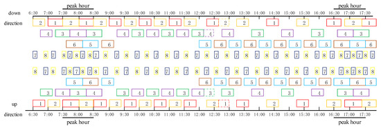
Figure 1.
Vehicle allocation and charging planning.
The average travel time of short-turning buses is 9 min in the off-peak period, while the departure interval is 20 min in this period. Therefore, buses 7 and 8 have a long idle time between two consecutive operation trips. Consequently, a short-turning bus can meet the passenger demand in the off-peak period. However, the result is that two short-turning buses are dispatched alternately in view of the electricity costs. In this case, the SOC of each bus can be decreased slowly to weaken the electricity consumption and reduce electricity costs.
- (3)
- Vehicle charging scheme
Although short-turning buses have a long idle time in the off-peak period, they are not recharged, as shown in Figure 1. The reasons behind this are that the electric power of the bus can meet the operation of the whole day, and the electricity cost of overnight charging is less than that of the combinational charging tactic. Furthermore, all-stop buses are recharged from 12:00 to 13:30, which is in the semi-peak prices and the off-peak period of passenger flow. It is reasonable to be recharged at that period from the perspective of minimizing the total cost of public transportation.
4.3. Schemes Comparison
- (1)
- Total costs comparison
The combinational scheduling has an impact on the passenger travel time costs, vehicle depreciation costs, and electricity costs, as shown in Figure 2. The blue histogram depicts the costs when all-stop scheduling is adopted, and the red histogram shows the cost under combinational scheduling strategy of all-stop and short-turning scheduling.
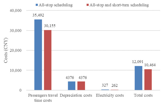
Figure 2.
Costs when using all-stop scheduling and combinational scheduling.
The passengers travel time costs in the whole day are reduced from 35,492 CNY to 30,155 CNY, with a decreasing rate of 15.1%. Vehicles are recharged during the semi-peak prices, which increases SOC and makes the electricity consumption reduce slowly. The electricity cost is 326 CNY when an overnight charging strategy is adopted, while it is 262 CNY under the charging strategy of combining daytime and overnight. The reduction of the electricity costs is 19.5%. Compared with all-stop scheduling, the total costs are reduced from 12,091 CNY to 10,464 CNY, dropping by 13.5%.
- (2)
- Weight analysis
Since the objective function is the weighted sum of the three indexes (passenger travel time costs, electricity costs, and depreciation costs), the total objective function value will also change as weights are adjusted. When the weight of the passenger travel time cost is a fixed value, which is 0.3, that of the public transport corporation cost is 0.7. Considering the impact of vehicle depreciation costs and electricity costs on the bus company cost, the weights of both of them are analyzed, as shown in Figure 3.
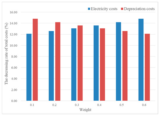
Figure 3.
Changes of weight factor, which is related to the electricity cost and depreciation cost.
Figure 3 demonstrates the effects of various weights of electricity cost and depreciation cost on the total cost. Obviously, with the increasing of the weight of depreciation cost, the decreasing rate of the total cost reduces to the minimum (12.1%) gradually. Meanwhile, it starts to rise slowly as the weight of the electricity cost increases. The largest decreasing rate of total costs is 14.8% when the weight of the electricity cost and depreciation cost are 0.6 and 0.1, respectively.
5. Conclusions
In this research, we develop the combinational short-turning and all-stop bus scheduling strategy, which enables an effective allocation of public transport resources to match the number of public transport vehicles with passenger demand on the line. The combinational strategy leads to a 15.1% decline in the total passenger travel time cost. In terms of charging strategy, our work leverages on the combination charging strategy to take advantage of semi-peak electricity prices in the daytime, reducing the electricity cost of the whole day by 19.5%. Generally, it is practical to establish the combinational strategy because the total cost, which is the weighted sum of the total passenger travel time costs, electricity costs, and vehicle depreciation costs, has been saved by 13.5%.
The branch-and-pricing algorithm used in this paper is a combination of the column generation algorithm and branch-and-bound method. We mainly apply the column generation algorithm to decompose the schemes of the whole vehicles into those of each vehicle and then solve them. The branch-and-bound method aims to obtain the integer solution, and then the vehicle scheduling and charging strategies are obtained. The branch-and-pricing algorithm is a kind of accurate solution method, which can find the exact solution better than a heuristic algorithm, but the calculation speed is relatively slow. Since the charging process is regarded as a virtual trip, the dimension of the initial solution is very large, leading to a slow calculation speed. The combination of branch-and-pricing algorithm and heuristic algorithm could be taken into account to further improve the calculation speed of the algorithm in future research.
The results show that the combinational scheduling strategy could reduce the passengers travel time cost and improve passenger satisfaction. Meanwhile, a charging strategy combining daytime with overnight can not only ensure the normal operation of the line with sufficient buses but also make full use of off-peak electricity prices to charge buses, so as to reduce electricity cost. The optimal result of charging strategy guides the bus company to opt a suitable time to charge electric buses for minimizing charging cost.
Although these results prove that the combinational scheduling strategy and charging planning proposed contribute to less passenger travel time cost and charging cost, to some extent, there are still some limitations; i.e., the combination of all-stop and short-turning strategies is not suitable to all bus lines, but merely for the bus lines for which passenger flow is uneven over space and more concentrated in some continuous stops.
In the future, we will establish a more general approach to address the problem that bus resources cannot match with the passenger demand of some stops.
Author Contributions
Conceptualization, Y.B., M.H. and M.G.; and methodology, Y.B. and M.H.; validation, Y.B., M.H. and M.G.; investigation, M.G.; writing—original draft preparation, M.G. and M.H.; writing—review and editing, Y.B. and M.G.; visualization, M.G.; supervision, Y.B.; funding acquisition, Y.B. All authors have read and agreed to the published version of the manuscript.
Funding
This research was funded by [Graduate Innovation Fund of Jilin University] grant number [101832020CX154], [National Natural Science Foundation of China] grant number [71771062 & 52002143], [China Postdoctoral Science Foundation] grant number [2019M661214 & 2020T130240], and [Fundamental Research Funds for the Central Universities].
Institutional Review Board Statement
Not applicable.
Informed Consent Statement
Not applicable.
Data Availability Statement
The data presented in this study are available on request from the corresponding author.
Conflicts of Interest
The authors declared that they have no conflict of interest to this work.
References
- Wang, J.; Kang, L.; Liu, Y. Optimal scheduling for electric bus fleets based on dynamic programming approach by considering battery capacity fade. Renew. Sustain. Energy Rev. 2020, 130, 9978. [Google Scholar] [CrossRef]
- Quttineh, N.H.; Häll, C.H.; Ekström, J.; Ceder, A. Combined Timetabling and Vehicle Scheduling for Electric Buses. In Proceedings of the 22nd International Conference of Hong Kong Society for Transportation Studies (HKSTS), Hong Kong, China, 9–11 December 2017. [Google Scholar]
- Wang, Y.; Huang, Y.; Xu, J.; Barclay, N. Optimal recharging scheduling for urban electric buses: A case study in Davis. Transp. Res. Part E Logist. Transp. Rev. 2017, 100, 115–132. [Google Scholar] [CrossRef]
- Guedes, P.C.; Borenstein, D. Column generation based heuristic framework for the multiple-depot vehicle type scheduling problem. Comput. Ind. Eng. 2015, 90, 361–370. [Google Scholar] [CrossRef]
- Gong, L.; Li, Y.; Xu, D. Combinational Scheduling Model Considering Multiple Vehicle Sizes. Sustainability 2019, 11, 5144. [Google Scholar] [CrossRef]
- Perumal, S.; Dollevoet, T.; Huisman, D.; Lusby, R.; Larsen, J.; Riis, M. Solution Approaches for Vehicle and Crew Scheduling with Electric Buses. Econometric Institute Research Papers. Available online: https://repub.eur.nl/pub/123963 (accessed on 4 January 2021).
- Gao, L. Research and application of vehicle bus combined scheduling model for urban public interval bus. Dalian Maritime University. 2017. Available online: http://cdmd.cnki.com.cn/Article/CDMD-10151-1017196186.htm (accessed on 4 January 2021).
- Cortés, C.E.; Díaz, J.S.; Tirachini, A. Integrating short turning and deadheading in the optimization of transit services. Transp. Res. Part A Policy Pract. 2011, 45, 419–434. [Google Scholar] [CrossRef]
- Ke, B.R.; Chung, C.Y.; Chen, Y.C. Minimizing the costs of constructing an all plug-in electric bus transportation system: A case study in Penghu. Appl. Energy 2016, 177, 649–660. [Google Scholar] [CrossRef]
- Bellei, G.; Gkoumas, K. Transit vehicles’ headway distribution and service irregularity. Public Transp. 2010, 2, 269–289. [Google Scholar] [CrossRef]
- Borndörfer, R.; Grötschel, M.; Pfetsch, M.E. A column-generation approach to line planning in public transport. Transp. Sci. 2007, 41, 123–132. [Google Scholar] [CrossRef]
- Ghaemi, N.; Cats, O.; Goverde, R.M.P. A microscopic model for optimal train short-turnings during complete blockages. Transp. Res. Part B Methodol. 2017, 105, 423–437. [Google Scholar] [CrossRef]
- Ji, Y.; Yang, X.; Du, Y. Optimal design of a short-turning strategy considering seat availability. J. Adv. Transp. 2016, 50, 1554–1571. [Google Scholar] [CrossRef]
- Canca, D.; Barrena, E.; Laporte, G.; Ortega, F.A. A short-turning policy for the management of demand disruptions in rapid transit systems. Ann. Oper. Res. 2016, 246, 145–166. [Google Scholar] [CrossRef]
- Carosi, S.; Frangioni, A.; Galli, L.; Girardi, L.; Vallese, G. A matheuristic for integrated timetabling and vehicle scheduling. Transp. Res. Part B Methodol. 2019, 127, 99–124. [Google Scholar] [CrossRef]
- Shang, H.Y.; Huang, H.J.; Wu, W.X. Bus timetabling considering passenger satisfaction: An empirical study in Beijing. Comput. Ind. Eng. 2019, 135, 1155–1166. [Google Scholar] [CrossRef]
- Zhang, Y.; Hu, Q.; Meng, Z.; Ralescu, A. Fuzzy dynamic timetable scheduling for public transit. Fuzzy Sets Syst. 2020, 395, 235–253. [Google Scholar] [CrossRef]
- Zhang, S.; Ceder, A.A.; Cao, Z. Integrated optimization for feeder bus timetabling and procurement scheme with consideration of environmental impact. Comput. Ind. Eng. 2020, 145, 6501. [Google Scholar] [CrossRef]
- Peña, D.; Tchernykh, A.; Nesmachnow, S.; Massobrio, R.; Feoktistov, A.; Bychkov, I.; Garichev, S.N. Operating cost and quality of service optimization for multi-vehicle-type timetabling for urban bus systems. J. Parallel Distrib. Comput. 2019, 133, 272–285. [Google Scholar] [CrossRef]
- Gkiotsalitis, K.; Alesiani, F. Robust timetable optimization for bus lines subject to resource and regulatory constraints. Transp. Res. Part E Logist. Transp. Rev. 2019, 128, 30–51. [Google Scholar] [CrossRef]
- Wang, C.; Shi, H.; Zuo, X. A multi-objective genetic algorithm based approach for dynamical bus vehicles scheduling under traffic congestion. Swarm Evol. Comput. 2020, 54, 667. [Google Scholar] [CrossRef]
- Zhang, C.; Chen, P. Economic benefit analysis of battery charging and swapping station for pure electric bus based on differential power purchase policy: A new power trading model. Sustain. Cities Soc. 2021, 64, 2570. [Google Scholar] [CrossRef]
- Gao, K.; Yang, Y.; Li, A.; Li, J.; Yu, B. Quantifying economic benefits from free-floating bike-sharing systems: A trip-level inference approach and city-scale analysis. Transp. Res. Part A Policy Pract. 2021, 144, 89–103. [Google Scholar] [CrossRef]
- Xu, Y.; Zheng, Y.; Yang, Y. On the movement simulations of electric vehicles: A behavioral model-based approach. Appl. Energy 2020, 6356. [Google Scholar] [CrossRef]
- Gao, K.; Yang, Y.; Sun, L.; Qu, X. Revealing psychological inertia in mode shift behavior and its quantitative influences on commuting trips. Transp. Res. Part F Traffic Psychol. Behav. 2020, 71, 272–287. [Google Scholar] [CrossRef]
- Teng, J.; Chen, T.; Fan, W.D. Integrated Approach to Vehicle Scheduling and Bus Timetabling for an Electric Bus Line. J. Transp. Eng. Part A Syst. 2020, 146, 9073. [Google Scholar] [CrossRef]
- Ke, B.R.; Lin, Y.H.; Chen, H.Z.; Fang, S.C. Battery charging and discharging scheduling with demand response for an electric bus public transportation system. Sustain. Energy Technol. Assess. 2020, 40, 741. [Google Scholar] [CrossRef]
- Tang, X.; Lin, X.; He, F. Robust scheduling strategies of electric buses under stochastic traffic conditions. Transp. Res. Part C Emerg. Technol. 2019, 105, 163–182. [Google Scholar] [CrossRef]
- Alwesabi, Y.; Wang, Y.; Avalos, R.; Liu, Z. Electric bus scheduling under single depot dynamic wireless charging infrastructure planning. Energy 2020, 213, 8855. [Google Scholar] [CrossRef]
- Häll, C.H.; Ceder, A.; Ekström, J.; Quttineh, N.H. Adjustments of public transit operations planning process for the use of electric buses. J. Intell. Transp. Syst. 2019, 23, 216–230. [Google Scholar] [CrossRef]
- Rinaldi, M.; Parisi, F.; Laskaris, G.; Ariano, D.A.; Viti, F. Optimal dispatching of electric and hybrid buses subject to scheduling and charging constraints. In Proceedings of the 2018 21st International Conference on Intelligent Transportation Systems (ITSC), Maui, HI, USA, 4–7 November 2018; pp. 41–46. [Google Scholar]
- Zhang, L.; Zeng, Z.; Qu, X. On the Role of Battery Capacity Fading Mechanism in the Lifecycle Cost of Electric Bus Fleet. IEEE Trans. Intell. Transp. Syst. 2020. [Google Scholar] [CrossRef]
- Bie, Y.; Xiong, X.; Yan, Y.; Qu, X. Dynamic headway control for high-frequency bus line based on speed guidance and intersection signal adjustment. Comput. Aided Civil Infrastruct. Eng. 2020, 35, 4–25. [Google Scholar] [CrossRef]
- Wang, S.; Zhang, W.; Bie, Y.; Wang, K.; Diabat, A. Mixed-integer second-order cone programming model for bus route clustering problem. Transp. Res. Part C Emerg. Technol. 2019, 102, 351–369. [Google Scholar] [CrossRef]
- Ma, D.; Xiao, J.; Song, X.; Ma, X.; Jin, S. A back-pressure-based model with fixed phase sequences for traffic signal optimization under oversaturated networks. IEEE Trans. Intell. Transp. Syst. 2020. [Google Scholar] [CrossRef]
- Gkiotsalitis, K.; Wu, Z.; Cats, O. A cost-minimization model for bus fleet allocation featuring the tactical generation of short-turning and interlining options. Transp. Res. Part C Emerg. Technol. 2019, 98, 14–36. [Google Scholar] [CrossRef]
- Cao, Z.; Ceder, A.A. Autonomous short-turning bus service timetabling and vehicle scheduling using skip-stop tactic. Transp. Res. Part C Emerg. Technol. 2019, 102, 370–395. [Google Scholar] [CrossRef]
- Chen, J.; Liu, Z.; Wang, S.; Chen, X. Continuum approximation modeling of transit network design considering local route service and short-turn strategy. Transp. Res. Part E Logist. Transp. Rev. 2018, 119, 165–188. [Google Scholar] [CrossRef]
- Zhang, H.; Zhao, S.; Liu, H.; Liang, S. Design of integrated limited-stop and short-turn services for a bus route. Math. Probl. Eng. 2016, 2016. [Google Scholar] [CrossRef]
- Tirachini, A.; Cortés, C.E.; Díaz, J.S.R. Optimal design and benefits of a short-turning strategy for a bus corridor. Transportation 2011, 38, 169–189. [Google Scholar] [CrossRef]
- Ma, D.; Song, X.; Li, P. Daily traffic flow forecasting through a contextual convolutional recurrent neural network modeling inter-and intra-day traffic patterns. IEEE Trans. Intell. Transp. Syst. 2020. [Google Scholar] [CrossRef]
- Ma, D.; Xiao, J.; Ma, X. A decentralized model predictive traffic signal control method with fixed phase sequence for urban networks. J. Intell. Transp. Syst. 2020. [Google Scholar] [CrossRef]
- Wolbertus, R.; Van den Hoed, R. Electric vehicle fast charging needs in cities and along corridors. World Electr. Veh. J. 2019, 10, 45. [Google Scholar] [CrossRef]
- Rogge, M.; van der Hurk, E.; Larsen, A.; Sauer, D.U. Electric bus fleet size and mix problem with optimization of charging infrastructure. Appl. Energy 2018, 211, 282–295. [Google Scholar] [CrossRef]
- Rupp, M.; Rieke, C.; Handschuh, N.; Kuperjans, I. Economic and ecological optimization of electric bus charging considering variable electricity prices and CO2eq intensities. Transp. Res. Part D Transp. Environ. 2020, 81, 2293. [Google Scholar] [CrossRef]
- Yang, Y.; Yao, E.; Yang, Z.; Zhang, R. Modeling the charging and route choice behavior of BEV drivers. Transp. Res. Part C Emerg. Technol. 2016, 65, 190–204. [Google Scholar] [CrossRef]
- Lin, Y.; Zhang, K.; Shen, Z.J.M.; Ye, B.; Miao, L. Multistage large-scale charging station planning for electric buses considering transportation network and power grid. Transp. Res. Part C Emerg. Technol. 2019, 107, 423–443. [Google Scholar] [CrossRef]
- An, K. Battery electric bus infrastructure planning under demand uncertainty. Transp. Res. Part C Emerg. Technol. 2020, 111, 572–587. [Google Scholar] [CrossRef]
- He, Y.; Song, Z.; Liu, Z. Fast-charging station deployment for battery electric bus systems considering electricity demand charges. Sustain. Cities Soc. 2019, 48, 1530. [Google Scholar] [CrossRef]
- Chen, L.; Qian, K.; Qin, M.; Xu, X.; Xia, Y. A Configuration-Control Integrated Strategy for Electric Bus Charging Station With Echelon Battery System. IEEE Trans. Ind. Appl. 2020, 56, 6019–6028. [Google Scholar] [CrossRef]
- Chen, G.; Hu, D.; Chien, S. Optimizing battery-electric-feeder service and wireless charging locations with nested genetic algorithm. IEEE Access 2020, 8, 67166–67178. [Google Scholar] [CrossRef]
- Xu, M.; Yang, H.; Wang, S. Mitigate the range anxiety: Siting battery charging stations for electric vehicle drivers. Transp. Res. Part C Emerg. Technol. 2020, 114, 164–188. [Google Scholar] [CrossRef]
- Qin, N.; Gusrialdi, A.; Brooker, R.P.; Ali, T. Numerical analysis of electric bus fast charging strategies for demand charge reduction. Transp. Res. Part A Policy Pract. 2016, 94, 386–396. [Google Scholar] [CrossRef]
- He, Y.; Liu, Z.; Song, Z. Optimal charging scheduling and management for a fast-charging battery electric bus system. Transp. Res. Part E Logist. Transp. Rev. 2020, 142, 2056. [Google Scholar] [CrossRef]
- Wang, G.; Xie, X.; Zhang, F.; Liu, Y.; Zhang, D. bCharge: Data-driven real-time charging scheduling for large-scale electric bus fleets. In Proceedings of the 2018 IEEE Real-Time Systems Symposium (RTSS), Nashville, TN, USA, 11–14 December 2018; pp. 45–55. [Google Scholar]
- Barnhart, C.; Johnson, E.L.; Nemhauser, G.L.; Savelsbergh, M.W.P.; Vance, P.H. Branch-and-price: Column generation for solving huge integer programs. Oper. Res. 1998, 46, 316–329. [Google Scholar] [CrossRef]
- Tian, S. Study on Multi-Mode Bus Frequency Allocation Based on Stop Demand Elasticity; Chang’an University: Xi’an, China, 2017. [Google Scholar]
- Guo, C.; Wang, C.; Zuo, X. A genetic algorithm based column generation method for multi-depot electric bus vehicle scheduling. In Proceedings of the Genetic and Evolutionary Computation Conference Companion, New York, NY, USA, 9–13 July 2019; pp. 367–368. [Google Scholar]


Publisher’s Note: MDPI stays neutral with regard to jurisdictional claims in published maps and institutional affiliations. |
© 2021 by the authors. Licensee MDPI, Basel, Switzerland. This article is an open access article distributed under the terms and conditions of the Creative Commons Attribution (CC BY) license (http://creativecommons.org/licenses/by/4.0/).