
Data Model for Residential and Commercial Buildings. Load Flexibility Assessment in Smart Cities


Abstract
1. Introduction and Literature Review
2. Data Processing Methodology
- Date/Time
- Electricity: Facility
- Gas: Facility
- Heating: Electricity
- Heating: Gas
- Cooling: Electricity
- HVAC Fans: Electricity
- General, Interior Lights: Electricity
- General, Exterior Lights: Electricity
- Appl., Interior Equipment: Electricity
- Misc., Interior Equipment: Electricity
- Water Heater and Water Systems: Gas
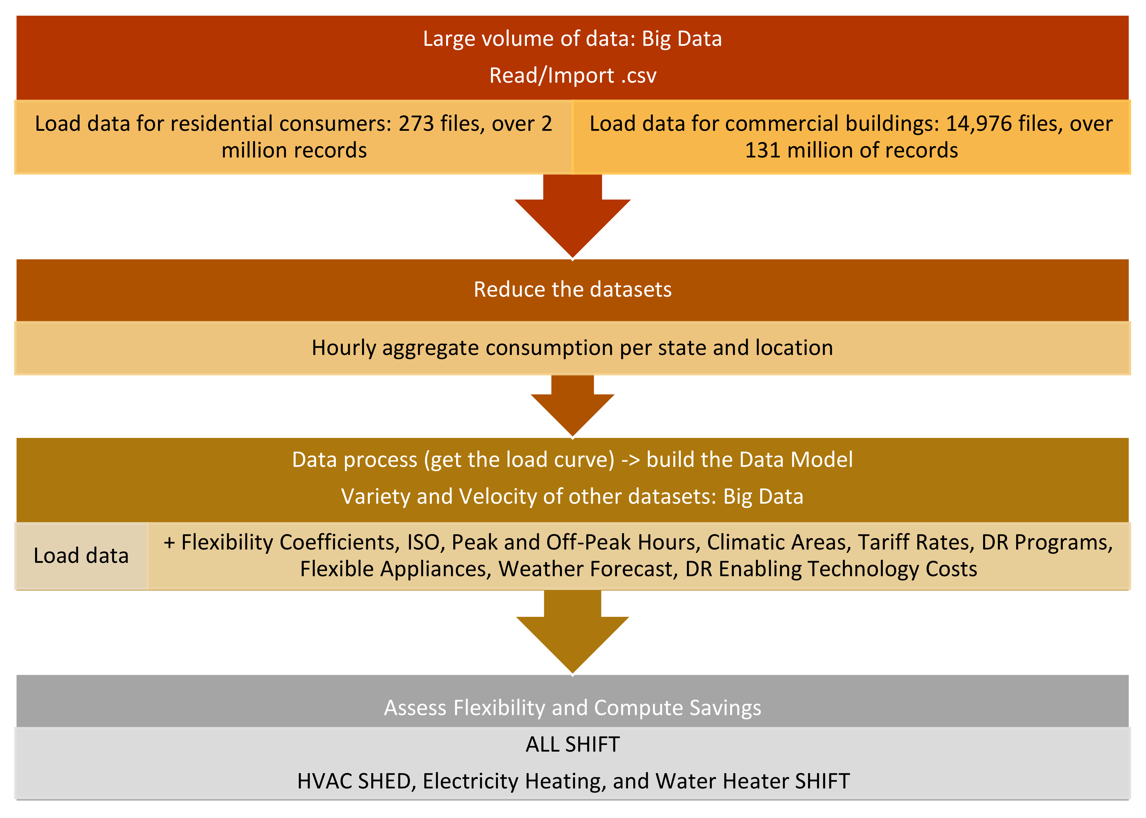
- Only .csv files were analyzed as input datasets, so the data presentation was standard;
- All the .csv files had the same fields/columns structure (Date/Time, Electricity: Facility, Fans: Electricity, Cooling: Electricity, Heating: Electricity, InteriorLights: Electricity, InteriorEquipment: Electricity, Gas: Facility, Heating: Gas, InteriorEquipment: Gas, Water Heater: WaterSystems: Gas);
- Each file name had a pattern which could give us more information about the dataset, as an example for RefBldgLargeHotelNew2004_v1.3_7.1_3A_USA_GA_ATLANTA.csv, the pattern is Ref [LocationType][Year]_v1.3_7.1_3A_[Country]_[State_ISO]_[City].csv. Location type, year, country, state independent system operator (ISO) and city are vital information extracted them for each file;
- The structure of the file path was easy to scan after unzipping each archive. An example is COMMERCIAL_LOAD_DATA_E_PLUS_OUTPUT.part9\USA_TX_Alice.Intl.AP.722517_TMY3\RefBldgStripMallNew2004_v1.3_7.1_2A_USA_TX_HOUSTON.csv having the following pattern [ARHIVE_NAME]\[ROOT_FOLDER]\[FILE_NAME].csv.
- ○
- Scalable with a big data load;
- ○
- Familiar and easy to use;
- ○
- Can run on local machines;
- ○
- Easy to setup;
- ○
- Open Source.
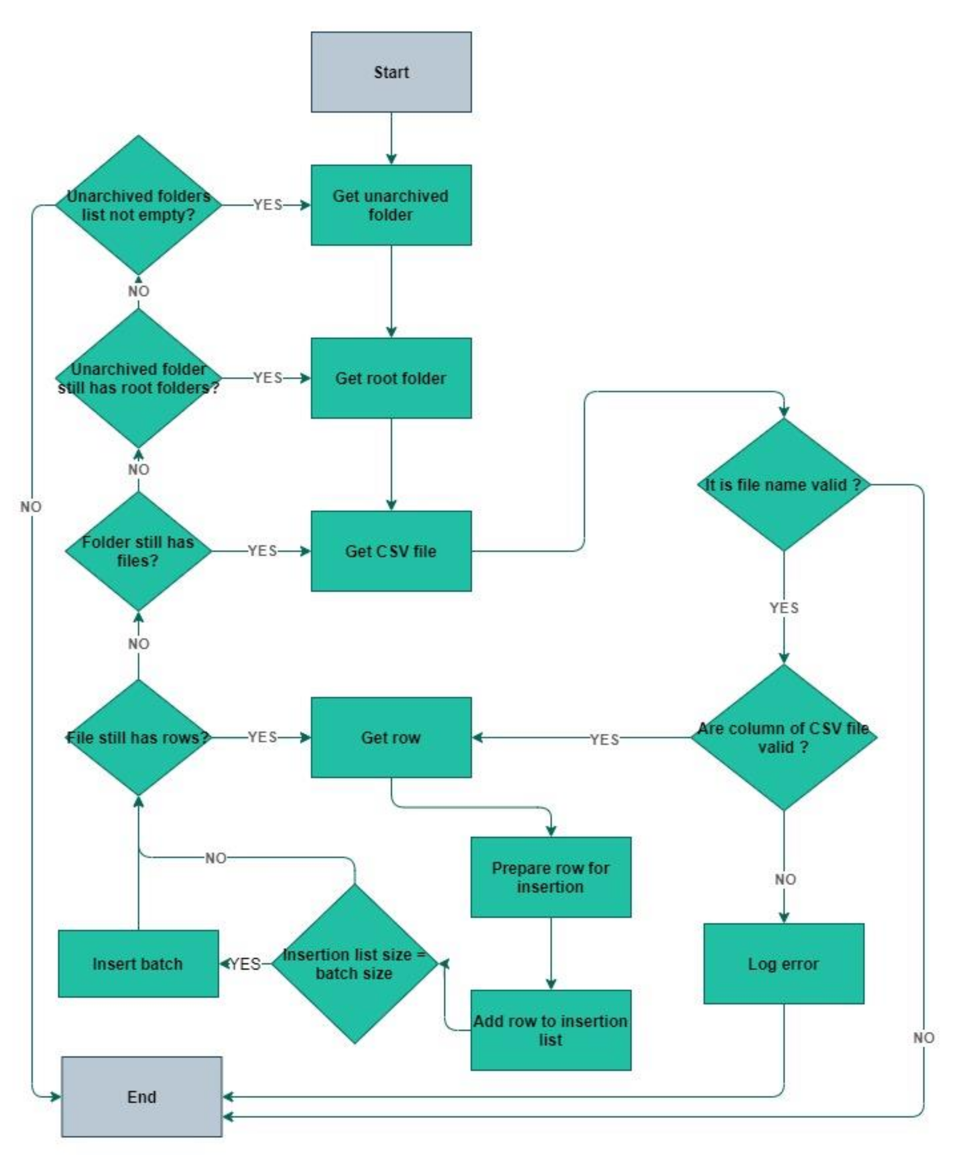
- The script starts scanning the target path for unarchived data folders (prerequisite step was to download all the archived data and unarchived it to a specific path).
- The script finds an unarchived folder and scans it inside for a root data folder.
- The script finds a root data folder and starts to iterate on each file. At this point, the files are in .csv format.
- Each file is opened, and the columns of .csv format are validated. In case a column is missing, or an unexpected column appears the script will log an error and close the process. In this way, an inconsistency can easily be identified and investigated.
- If the columns are valid the script will iterate though the rows. The columns of file will be combined with the row values and each row data will be added to the “rows to be inserted” list.
- If the number of items in list is equals to the number of batch size (to be inserted), the list will be transformed into a big batch statement and ran against the PostgreSQL database.
- If the end of file is reached and the number of rows to be inserted is not equals to the number of batch size, the insert will be done, so it can be continued with another file.
- The next file will be processed.
- If the root folder has no more file, the root folder will be changed.
- If the unarchived folder has no more root folders, the unarchived folder will be changed.
- The program will end when there will be no more unarchived folders to be processed.
3. Building the Data Model and Algorithm for Load Flexibility Assessment
3.1. DR Capability, Climatic Areas, and ISO
3.2. DR Programs
3.3. DR Enabling Technology Costs
3.4. Weather Data and Flexibility Forecast
3.5. Data Model
3.6. Algorithm for Load Flexibility Assessment
4. Simulations and Results
5. Conclusions
Author Contributions
Funding
Institutional Review Board Statement
Informed Consent Statement
Data Availability Statement
Conflicts of Interest
Abbreviations
| DR | Demand Response |
| RES | Renewable Energy Sources |
| EV | Electric Vehicle |
| ISO | Independent System Operator |
| DLC | Direct Load Control |
| PCT | Programmable Communicating Thermostat |
| ADR | Automated Demand Response |
| HVAC | Heating, Ventilation, and Air Conditioning |
| SASM | Smart Adaptive Switching Module |
| EH | Electricity Heating |
| WH | Water Heater |
| ToU | Time-of-Use |
| Hour | |
| Peak start hour | |
| Peak stop hour | |
| Flexible capacity; | |
| Flexibility coefficient; | |
| Consumption of electricity heating | |
| Consumption of water heater | |
| Consumption of HVAC | |
| Savings from flexibility usage | |
| Tariff rate at peak hours | |
| Tariff rate at off-peak hours |
References
- Hledik, R.; Faruqui, A.; Lee, T.; Higham, J. The National Potential for Load Flexibility: Value and Market Potential through 2030. Available online: https://brattlefiles.blob.core.windows.net/files/16639_national_potential_for_load_flexibility_-_final.pdf (accessed on 2 November 2020).
- D’hulst, R.; Labeeuw, W.; Beusen, B.; Claessens, S.; Deconinck, G.; Vanthournout, K. Demand response flexibility and flexibility potential of residential smart appliances: Experiences from large pilot test in Belgium. Appl. Energy 2015, 155, 79–90. [Google Scholar] [CrossRef]
- Klaassen, E.A.M.; Kobus, C.B.A.; Frunt, J.; Slootweg, J.G. Responsiveness of residential electricity demand to dynamic tariffs: Experiences from a large field test in the Netherlands. Appl. Energy 2016, 183, 1065–1074. [Google Scholar] [CrossRef]
- Lopes, R.A.; Chambel, A.; Neves, J.; Aelenei, D.; Martins, J. A Literature Review of Methodologies Used to Assess the Energy Flexibility of Buildings. Energy Procedia 2016, 91, 1053–1058. [Google Scholar] [CrossRef]
- Reynders, G.; Amaral Lopes, R.; Marszal-Pomianowska, A.; Aelenei, D.; Martins, J.; Saelens, D. Energy flexible buildings: An evaluation of definitions and quantification methodologies applied to thermal storage. Energy Build. 2018, 166, 372–390. [Google Scholar] [CrossRef]
- Klaassen, E.A.M.; van Gerwen, R.J.F.; Frunt, J.; Slootweg, J.G. A methodology to assess demand response benefits from a system perspective: A Dutch case study. Util. Policy 2017, 44, 25–37. [Google Scholar] [CrossRef]
- Potter, J.; Cappers, P. Demand Response Advanced ControlsFramework and Assessment of Enabling Technology Costs. Available online: https://emp.lbl.gov/sites/default/files/demand_response_advanced_controls_framework_and_cost_assessment_final_published.pdf (accessed on 2 November 2020).
- Söder, L.; Lund, P.D.; Koduvere, H.; Bolkesjø, T.F.; Rossebø, G.H.; Rosenlund-Soysal, E.; Skytte, K.; Katz, J.; Blumberga, D. A review of demand side flexibility potential in Northern Europe. Renew. Sustain. Energy Rev. 2018, 91, 654–664. [Google Scholar] [CrossRef]
- Rotger-Griful, S.; Jacobsen, R.H.; Nguyen, D.; Sørensen, G. Demand response potential of ventilation systems in residential buildings. Energy Build. 2016, 121, 1–10. [Google Scholar] [CrossRef]
- Müller, T.; Möst, D. Demand Response Potential: Available when Needed? Energy Policy 2018, 115, 181–198. [Google Scholar] [CrossRef]
- Arteconi, A.; Polonara, F. Assessing the demand side management potential and the energy flexibility of heat pumps in buildings. Energies 2018, 11, 1846. [Google Scholar] [CrossRef]
- Yin, R.; Kara, E.C.; Li, Y.; DeForest, N.; Wang, K.; Yong, T.; Stadler, M. Quantifying flexibility of commercial and residential loads for demand response using setpoint changes. Appl. Energy 2016, 177, 149–164. [Google Scholar] [CrossRef]
- Klein, K.; Herkel, S.; Henning, H.M.; Felsmann, C. Load shifting using the heating and cooling system of an office building: Quantitative potential evaluation for different flexibility and storage options. Appl. Energy 2017, 203, 917–937. [Google Scholar] [CrossRef]
- Diamantoulakis, P.D.; Kapinas, V.M.; Karagiannidis, G.K. Big Data Analytics for Dynamic Energy Management in Smart Grids. Big Data Res. 2015, 2, 94–101. [Google Scholar] [CrossRef]
- Wang, Y.; Chen, Q.; Kang, C.; Xia, Q. Clustering of Electricity Consumption Behavior Dynamics Toward Big Data Applications. IEEE Trans. Smart Grid 2016, 7, 2437–2447. [Google Scholar] [CrossRef]
- Muntean, M. Business intelligence issues for sustainability projects. Sustainability 2018, 10, 335. [Google Scholar] [CrossRef]
- Muntean, M.; Cabău, L.G.; Rînciog, V. Social Business Intelligence: A New Perspective for Decision Makers. Procedia Soc. Behav. Sci. 2014, 124, 562–567. [Google Scholar] [CrossRef]
- Wang, Y.; Chen, Q.; Hong, T.; Kang, C. Review of Smart Meter Data Analytics: Applications, Methodologies, and Challenges. IEEE Trans. Smart Grid 2019, 10, 3125–3148. [Google Scholar] [CrossRef]
- Nordic Countries of Ministers. Flexible Demand for Electricity and Power: Barriers and Opportunities; Nordic Energy Research: Oslo, Norway, 2017. [Google Scholar]
- Office of Energy Efficiency & Renewable Energy (EERE). Commercial and Residential Hourly Load Profiles for all TMY3 Locations in the United States. Available online: https://openei.org/datasets/dataset/commercial-and-residential-hourly-load-profiles-for-all-tmy3-locations-in-the-united-states (accessed on 30 October 2020).
- National Renewable Energy Laboratory Building America House Simulation Protocols. Available online: https://www.nrel.gov/docs/fy11osti/49246.pdf (accessed on 30 October 2020).
- mongoDB. Comparing MongoDB vs PostgreSQL. Available online: https://www.mongodb.com/compare/mongodb-postgresql (accessed on 30 October 2020).
- National Renewable Energy Laboratory, U.S. Department of Energy Commercial Reference Building Models of the National Building Stock. Available online: https://www.nrel.gov/docs/fy11osti/46861.pdf (accessed on 30 October 2020).


| Scalable with a Big Data Load | Familiar and Easy to Use | Can Run on Local Machines | Easy to Setup | Open Source | |
|---|---|---|---|---|---|
| PostgreSQL | Yes | Yes | Yes | Yes | Yes |
| MongoDB | Yes | Yes | Yes | Yes | Yes |
| Cassandra DB | Yes | Partial | Yes | Partial | Yes |
| Elasticsearch | Yes | Yes | Yes | Partial | Yes |
| HBase (Hadoop) | Yes | Partial | Yes | Partial | Yes |
| Column Name Database | Data Type Database | Source | Example | Observation |
|---|---|---|---|---|
| date_time | Timestamp | .csv file | 11 July 2004 21:00:00 | |
| Id | Serial | Unique identifier of row, auto generated | ||
| electricity_facility_kwhourly | Numeric | .csv file | 10.8926491824 | |
| fans_electricity_kwhourly | Numeric | .csv file | 32.0021175342 | |
| cooling_electricity_kwhourly | Numeric | .csv file | 15.1069992076 | |
| heating_electricity_kwhourly | Numeric | .csv file | 5.48122459637 | |
| gas_facility_kwmonthly | Numeric | .csv file | 1.8243253836 | |
| interiorlights_electricity_kwhourly | Numeric | .csv file | 1.0115996781 | |
| interiorequipment_electricity_kwhourly | Numeric | .csv file | 4.04639871239 | |
| gas_facility_kwhourly | Numeric | .csv file | 7.29730153440 | |
| heating_gas_kwhourly | Numeric | .csv file | 16.4436737891 | |
| electricity_facility_kwmonthly | Numeric | .csv file | 24.9203635340 | |
| interiorequipment_gas_kwhourly | Numeric | .csv file | 5.48122459637 | |
| water_heater_watersystems_gas_kwhourly | Numeric | .csv file | 0.5500053624 | |
| location_type | Text | .csv file name | RefBldgSmallOffice | Extracted from the file name |
| year | Numeric | .csv file name | 2004 | Extracted from the file name |
| state_code | Text | .csv file name | GA | Extracted from the file name |
| city | Text | .csv file name | ATLANTA | Extracted from the file name |
| filename | Text | .csv file name | RefBldgWarehouseNew2004_v1.3_7.1_3A_USA_GA_ATLANTA.csv | Used for investigations |
| filepath | Text | .csv file path | D:\stats\Data\COMMERCIAL_LOAD_DATA_E_PLUS_OUTPUT.part1\USA_AL_Troy.Air.Field.722267_TMY3\RefBldgWarehouseNew2004_v1.3_7.1_3A_USA_GA_ATLANTA.csv | Used for investigations, in case we found some irrelevant data we can go directly to file |
| hour | Numeric | data_time field | 23 | Used to optimize the queries |
| Number of Inserted Rows per Batch | Total Duration Seconds | Total Rows Inserted |
|---|---|---|
| 1 | 5270.980333328247 | 1,007,400 |
| 100 | 538.0430161952972 | 1,007,400 |
| 200 | 435.40850925445557 | 1,007,400 |
| 300 | 382.5205578804016 | 1,007,400 |
| 350 | 381.44075322151184 | 1,007,400 |
| 400 | 367.4466257095337 | 1,007,400 |
| 500 | 371.1627984046936 | 1,007,400 |
| 1000 | 412.53081250190735 | 1,007,400 |
| No. | DR Program | Description |
|---|---|---|
| 1 | ADR or DLC | Control of customers’ flexible appliances for DR purposes using an automated signal that triggers a specific response. |
| 2 | Smart-thermostats | Temperature is remotely controlled to reduce heating/cooling appliances usage at peak. |
| 3 | Discounted rates | Residential consumers reduce consumption to a specific level and get a discounted rate. |
| 4 | Bid load | Residential consumers bid the day-ahead curtailment program at 15 min-resolution. If their orders are executed, they must curtail and receive an additional payment. Otherwise, they will encounter a penalty that is usually mentioned in an agreement. |
| 5 | Signal tariffs | Static or dynamic signal rates that encourage the consumption at off-peak intervals. These tariffs can be designed as Time-of-Use (ToU) tariffs, critical peak, variable peak, real-time pricing, or dynamic tariff rates set by consumption optimization with game theory. |
| 6 | Consumers’ awareness | Residential consumers are aware of the load reductions requirements and behave accordingly without a financial incentive. Such programs are tailored to show the advantages and benefits of a certain behavior towards a sustainable consumption. |
| 7 | Charging batteries | Residential consumers are stimulated to charge batteries including EV during off-peak interval. |
| 8 | Thermal storage | Boilers and other similar appliances operate at off-peak hours. The boiler tanks preserve the water temperature. For commercial buildings, it can be extended to the ice processing. Thus, the water can be frozen at off-peak hours and provide cooling at peak hours. |
| 9 | Smart Adaptive Switching Module (SASM) | It automates the control of various appliances, including generation and storage. It is based on a priority of the appliances and control of the load with fuzzy rules. |
| 10 | Dispatchable load | The program requires more engagement from consumers. |
| No. | Action | DR Program | Flexible App. | Control Tech. and Comm. Cost ($/End-Use) |
|---|---|---|---|---|
| 1 | Shed | DLC | HVAC | 166 |
| Pool pump | 147 | |||
| Room AC | 75 | |||
| 2 | Shed and Shift | Smart-thermostat | HVAC | 279 |
| 3 | Shimmy | ADR Control | Water Heater | 2136 |
| DLC | Water Heater | 350 |
| No. | Action | DR Program | Flexible App. | Control Tech. Cost ($/kW) | Comm. & Hardware Cost ($/Site) |
|---|---|---|---|---|---|
| 1 | Shed | DLC | HVAC | 62 | 107 |
| 2 | Shed and Shift | ADR Control | HVAC | 242 | - |
| Refrigerated Warehouse | 289 | - | |||
| Smart-thermostat | HVAC | 171 | - | ||
| 3 | Shimmy | ADR Control | HVAC | 310 | 2066 |
| Refrigerated Warehouse | 289 | 2066 | |||
| Water Heater | 166 | 1000 |
| No. | Step |
|---|---|
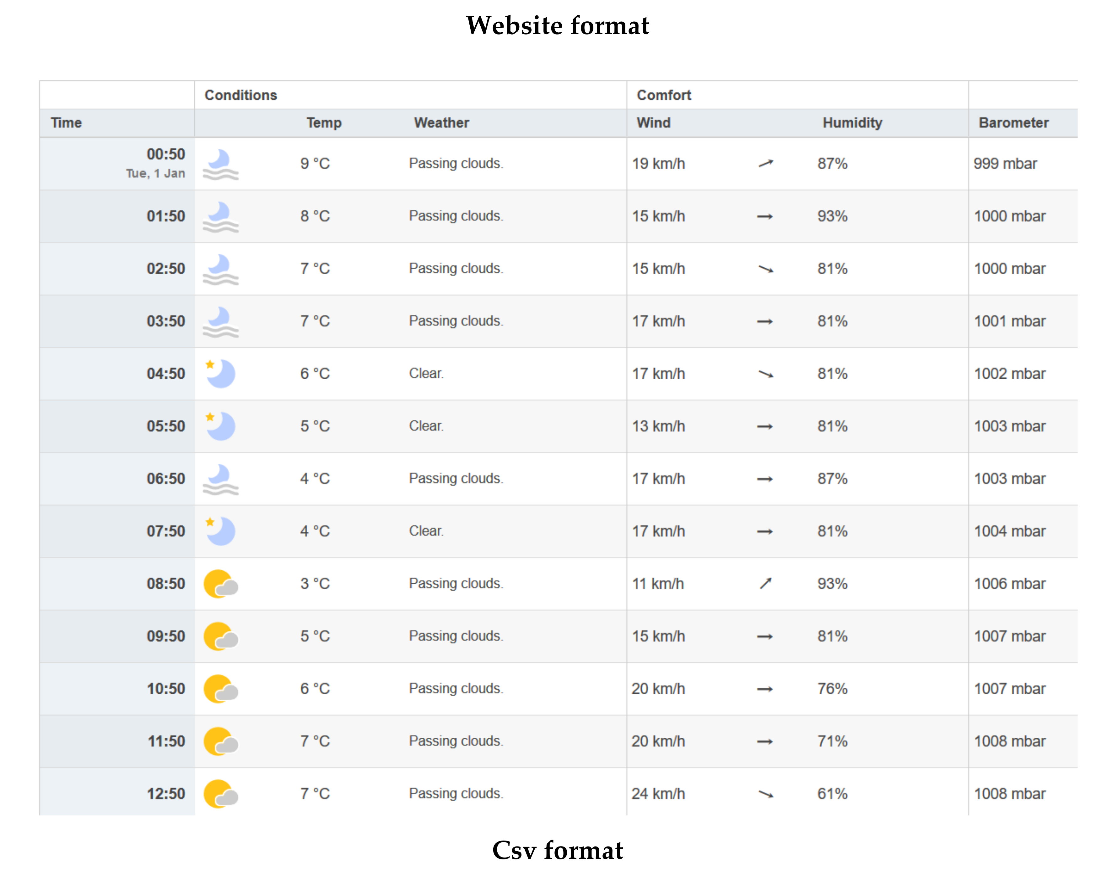
| 1 | //Using CURL PHP library to download data via HTTP //curl session initiation $ch = curl_init(); |
| 2 | //setting option with curl_setopt //CURLOPT_URL option to specify the URL curl_setopt ($ch, CURLOPT_URL, “https://www.timeanddate.com/scripts/cityajax.php?n=fl/states&mode=historic&hd={$data}&month={$dataMonth}&year={$dataYear}” (accessed on 2 February 2021)); //post request, 1-true curl_setopt ($ch, CURLOPT_POST, 1); //CURLOPT_RETURNTRANSFER returns the content of the page curl_setopt ($ch, CURLOPT_RETURNTRANSFER, true); |
| 3 | //execute session $ch and display the result in browser $server_output = curl_exec($ch); |
| 4 | //HtmlDomParser returns the content of the HTML page $dom = HtmlDomParser::str_get_html ($server_output); |
| 5 | //create and save the extracted data into a .csv file $fp = fopen (“Weather data {$dataAfisare}.csv”, ’w’); |
| Notations: —hour; —peak start hour; —peak stop hour; —flexible capacity; —flexibility coefficient; | —consumption of electricity heating; —consumption of water heater; —consumption of HVAC; —savings from flexibility usage; tariff rate at peak hours; tariff rate at off-peak hours. |
| Case 1: ALL SHIFT | Case 2: HVAC SHED, EH, WH SHIFT |
| Assess flexibility | Assess flexibility |
| Compute savings | Compute savings |
| Shifted Load (kWh) | Shed Load (kWh) | Savings (Euro) | |
|---|---|---|---|
| ALL SHIFT | 12,434.42 | 0 | 3605.98 |
| Total CASE1 | 12,434.42 | 0 | 3605.98 |
| EH SHIFT | 327.46 | 0 | 94.96 |
| WH SHIFT | 4025.12 | 0 | 1167.29 |
| HVAC SHED | 0.00 | 8081.84 | 3071.10 |
| Total CASE2 | 4352.58 | 8081.84 | 4333.35 |
Publisher’s Note: MDPI stays neutral with regard to jurisdictional claims in published maps and institutional affiliations. |
© 2021 by the authors. Licensee MDPI, Basel, Switzerland. This article is an open access article distributed under the terms and conditions of the Creative Commons Attribution (CC BY) license (http://creativecommons.org/licenses/by/4.0/).
Share and Cite
Oprea, S.-V.; Bâra, A.; Marales, R.C.; Florescu, M.-S. Data Model for Residential and Commercial Buildings. Load Flexibility Assessment in Smart Cities. Sustainability 2021, 13, 1736. https://doi.org/10.3390/su13041736
Oprea S-V, Bâra A, Marales RC, Florescu M-S. Data Model for Residential and Commercial Buildings. Load Flexibility Assessment in Smart Cities. Sustainability. 2021; 13(4):1736. https://doi.org/10.3390/su13041736
Chicago/Turabian StyleOprea, Simona-Vasilica, Adela Bâra, Răzvan Cristian Marales, and Margareta-Stela Florescu. 2021. "Data Model for Residential and Commercial Buildings. Load Flexibility Assessment in Smart Cities" Sustainability 13, no. 4: 1736. https://doi.org/10.3390/su13041736
APA StyleOprea, S.-V., Bâra, A., Marales, R. C., & Florescu, M.-S. (2021). Data Model for Residential and Commercial Buildings. Load Flexibility Assessment in Smart Cities. Sustainability, 13(4), 1736. https://doi.org/10.3390/su13041736