Machine Learning Aided Design and Prediction of Environmentally Friendly Rubberised Concrete

Abstract

Not only can waste rubber enhance the properties of concrete (e.g., its dynamic damping and abrasion resistance capacity), its rational utilisation can also dramatically reduce environmental pollution and carbon footprint globally. This study is the world’s first to develop a novel machine learning-aided design and prediction of environmentally friendly concrete using waste rubber, which can drive sustainable development of infrastructure systems towards net-zero emission, which saves time and cost. In this study, artificial neuron networks (ANN) have been established to determine the design relationship between various concrete mix composites and their multiple mechanical properties simultaneously. Interestingly, it is found that almost all previous studies on the ANNs could only predict one kind of mechanical property. To enable multiple mechanical property predictions, ANN models with various architectural algorithms, hidden neurons and layers are built and tailored for benchmarking in this study. Comprehensively, all three hundred and fifty-three experimental data sets of rubberised concrete available in the open literature have been collected. In this study, the mechanical properties in focus consist of the compressive strength at day 7 (CS7), the compressive strength at day 28 (CS28), the flexural strength (FS), the tensile strength (TS) and the elastic modulus (EM). The optimal ANN architecture has been identified by customising and benchmarking the algorithms (Levenberg–Marquardt (LM), Bayesian Regularisation (BR) and Scaled Conjugate Gradient (SCG)), hidden layers (1–2) and hidden neurons (1–30). The performance of the optimal ANN architecture has been assessed by employing the mean squared error (MSE) and the coefficient of determination ($R^2)$. In addition, the prediction accuracy of the optimal ANN model has ben compared with that of the multiple linear regression (MLR).

1. Introduction

Rubber or elastomer is a common material and is widely used as an essential material in the manufacture of tires. Because the demand for rubber has continued to increase over time, the global consumption of rubber in 2017 was 13,225 thousand metric tons of natural rubber and 15,189 thousand metric tons of synthetic rubber [1]. The generation of waste rubber in the EU is estimated to be more than 1.43 billion tons per year and has been growing at a rate comparable to the EU’s economic growth. Nearly 5 billion tires, including stacked tires, will have been discarded by 2030 [2]. Thus, the utilisation of waste rubber resources is seen as an effective method for reducing their adverse effects on the environment, maintaining natural resources and reducing the demand for storage space [3]. At present, the main methods for the disposal of waste rubber are incineration and burial. There is a detrimental effect on the environment when waste rubber is burned because of the emissions of carbon dioxide and cyanide. According to the American Rubber Manufacturers Association Report, only approximately 5.5% of waste rubber is used for civil engineering. If more waste rubber is reused, more resources can be saved and negative effects on the environment can be reduced. As the primary source of waste rubber, scrapped tires, being an important waste material, have been studied and examined in relation to the field of construction [4]. The application of discarded automobile rubber tires in the civil engineering industry can be traced back to the last century. Waste rubber tires mainly ended up in landfill or were used as cushioning materials until the 1960s when rubber tires began to be used on a large scale in the construction industry due to the increasing amount of waste and enhanced environmental protection plans [5]. Therefore, waste rubber is now used as a substitute for aggregates (as either fine or coarse aggregates). When using discarded rubber tires to wholly or partially replace fine aggregates, the resulting concrete is lighter in weight. By using rubber tires instead of coarse aggregates, the elasticity and energy absorption capacity of the concrete are increased accordingly [6,7]. Moreover, the shrinkage of rubberised concrete increases with the increase in rubber sand content [8]. Research articles have shown a growth in the noise reduction coefficient with an increase in rubber replacing sand. Therefore, replacing aggregates with waste rubber in concrete at an opportune ratio not only supports the improvement of the performance of the concrete but also avoids the environmental pollution and waste of resources caused by conventional treatments [9,10]. The use of waste rubber can help engineers and stakeholders achieve a system’s zero emission status in a faster and safer manner. This practice will fundamentally underpin the United Nation’s sustainable development goals (SDGs) as well as the “race to zero” campaign.

Although there is a huge potential in the substitution of aggregates with waste rubber, the weakness in the mechanical properties and the durability of concrete due to the poor performance of rubber in bonding cement particles has been mentioned [11,12,13,14]. Thus, various methods for improving the durability and the mechanical properties of concrete have been proposed. For instance, the following treatments of rubber have been employed to improve the compressive strength of rubberised concrete: water soaking and washing, utilising rubber particles with large sizes, NaOH treatment, treatment with acetone or ethanol [15,16]. Furthermore, an innovative method, compression concrete casting, has been proposed to improve the compressive strength and elastic modulus of rubberised concrete. When 20% of the coarse aggregates in compressed concrete samples was replaced with rubber particles, the compressive strength and elastic modulus of the concrete were enhanced by 35% and 29%, respectively [17,18]. Regarding the flexural strength, the splitting tensile strength and the elastic modulus, the methods of water washing, water soaking and coating with cement paste were seen to enhance these properties. In order to obtain rubberised concrete with promising workability, rubber particles were added into a mixer with other concrete components, with the exception of water for dry mixing, and then water was added as the other components were mixed homogeneously [16].

Machine learning is often referred to as being part of the artificial intelligence used to analyse data to make smart decisions [19]. It is a method of realising artificial intelligence which has the ability to learn and predict data [20]. By adopting machine learning, it is possible to predict the performance of rubberised concretes that have different compositions. Machine learning can be developed by a variety of algorithms which are commonly classified into four different learning types according to their learning style: supervised, unsupervised, semi-supervised and reinforcement learning [21]. Supervised learning is suitable for data that have features and labels. In other words, data are provided to predict the labels. Unsupervised learning is only used in features with no labels, which means that data are provided to look for hidden structures. The difference between the above two styles is that supervised learning only uses labelled sample sets for learning, while unsupervised learning only uses unlabeled sample sets. For semi-supervised learning, some of the data are unlabelled, but most of it is labelled. Compared to supervised learning, the cost of semi-supervised learning is lower, but it can achieve higher accuracy. Reinforcement learning also uses unlabeled data, but it is possible to see whether it is getting closer or further away from the correct answer. In engineering design, computer-aided methods such as machine learning and data statistics have been effectively used and can provide powerful benefits [22], especially when dealing with materials with complex variables and high uncertainty, such as composite materials [23]. A number of studies have shown that machine learning models have been widely applied and used as valuable tools for the prediction of the mechanical properties of concrete [24,25,26].

An artificial neuron network (ANN), a type of machine learning, is a simplified mathematical model that can simulate the function of natural biological neural networks to learn from past experience for solving new problems [27,28]. Since a large amount of data, such as compositions and properties of concrete, needs to be processed, the ordinary statistical methods cannot be sufficiently applied to the prediction of concrete properties. Furthermore, the prediction accuracy of the ordinary statistical methods may not be satisfied without proper algorithmic support. Based on previous experimental results, ANN models were used for predicting the mix proportion of polymer concrete to demonstrate the potential in saving time and costs [27,29]. Moreover, an ANN model with one hidden layer and 11 hidden neurons was utilised for predicting the compressive strength of concrete containing silica fume; 0.9724 of the R² value indicating the high prediction accuracy of the ANN model was obtained. An acceptable MSE value of the ANN model employed for estimating the compressive strength and elastic modulus of lightweight concrete was also acquired [30]. Therefore, it is clear that ANN can be selected as the suitable training method for this study. According to the previous studies related to the ANN for concrete property prediction, it can be found that the ANN was employed for predicting only one output in almost all previous studies. However, in reality, multiple mechanical properties are often required as part of engineering design and technical specifications. If an ANN model can predict multiple outputs (i.e., mechanical properties) with a satisfactory prediction accuracy, the optimal design and prediction of the concrete properties can be established, resulting in a reduction in material wastes and unnecessary costs. Thus, it is essential to automate the concrete design and prediction, which can improve waste management strategies towards net-zero built environments.

A typical structure of the ANN is demonstrated in Figure 1. It usually consists of three parts, the input layer, the output layer, and one or more hidden layers. Each layer has different numbers of neurons linked together by connections. In order to improve the accuracy of an ANN model, it is generally recommended to set one and two hidden layers containing multiple neurons. Moreover, the weight consists of the sum of regression coefficients and bias. The corresponding weight of layers can be added to each connection. An ANN model can be optimised by adjusting the weight during the training process until the error is reduced to an acceptable level [31]. Furthermore, the sigmoid function can be applied as the active function to analyse the effect of input elements and the weight on this element being processed [32]. For an ANN model, the number of hidden layers, connections and neurons are confirmed by the complexity of the raw data. The more complex the raw data are, the more hidden layers and neurons there are [33]. In order to obtain a high-accuracy model, the number of hidden layers and neurons of the model can be modified and compared in this study.

The aim of this research is to establish a novel machine learning apporach capable of designing and predicting multiple mechanical properties of rubberised concrete with various compositions. The ANN models are found to be capable of managing the complicated relationships between the inputs and outputs and of designing rubberised concrete that enhances resource conservation and environment protection by decreasing the experimental cost. Firstly, 335 experimental data sets of rubberised concrete properties with different compositions have been collected from published articles in open literature. Subsequently, the ANN models with different architectures (1–2 hidden layers and 1–30 hidden neurons) have been designed utilising MATLAB. Then, the optimal ANN architecture can be determined, followed by the performance evaluation. Finally, the prediction accuracy of multiple linear regression (MLR) conducted in the comparative analysis section is compared with that of the optimal ANN architecture capable of designing and predicting multiple mechanical properties of rubberised concrete.

2. Materials and Methods

2.1. Data Collection

The data used in this research have been collected from published articles in the open literature. In order to import data into the machine learning model in MATLAB, two items of the data sets for the pre-treatment method of rubber have been replaced by digitisation numbers described in

Table 1. The representation of numbers for the pre-treatment rubber method.

Number	Representation
1	No special treatment
2	Pre-treated with NaOH
3	Pre-coated with limestone

. The data set size of the cement type and the ratio of rubber replacement are listed in

Table 2. The representation of numbers for the cement type.

Number	Representation
1	Portland Cement of Grade 32.5
2	CEMI High Strength Portland Cement (52.5 MPa)
3	Ordinary Portland Cement grade 42.5
4	ASTM C150 I (Ordinary Portland Cement Type I)
5	Portland Cement (42.5 MPa)
6	ASTM C150 II (Ordinary Portland Cement Type II)
7	AS 3972 for Type GB (Blended) cement

and

Table 3. The replaced ratios of rubber and the cement type.

Data Set Size	Cement Type	Replacement by Rubber	Reference
8	1	1%, 3%, 5%, 10%, 15%, 20%	[34]
3	2	3%, 5%, 8%	[35]
5	3	5%, 10%, 15%, 20%, 30%	[36]
12	4	5%, 10%, 15%, 20%	[37]
9	2	5%, 10%, 15%	[38]
27	5	5%, 10%, 15%, 20%, 25%, 30%	[39]
6	4	5%, 10%, 15%	[40]
8	4	5%, 10%, 15%, 20%	[41]
3	6	5%, 7.5%, 10%	[42]
9	3	5%, 10%, 20%	[43]
9	4	5%, 10%, 15%	[40]
3	5	5%, 10%, 15%	[44]
5	1	9%, 15%, 30%, 58.80%, 100%	[45]
9	4	10%, 20%, 30%	[46]
6	6	10%	[47]
10	4	25%, 50%, 75%, 100%	[48]
12	4	5%, 10%, 15%, 20%	[49]
9	7	20%	[50]
7	1	15%, 25%, 30%, 50%, 75%,	[51]
48	4	2.5%, 5%, 10%, 15%, 25%, 50%	[52]
24	1	5%, 10%, 15%, 25%, 30%, 40%, 50%	[53]
9	1	10%, 20%, 30%	[46]
11	4	5%, 10%, 15%, 20%, 40%	[54]
5	4	5%, 10%, 15%, 20%, 30%	[6]
5	5	20%, 40%, 60%, 80%, 100%	[55]
15	5	5%, 10%, 15%, 20%, 25%	[56]
4	4	10%, 20%, 30%, 40%	[57]
16	4	5%, 10%, 15%, 20%	[58]
4	3	4%, 4.5%, 5%, 5.5%	[59]
53	4	5%, 10%, 15%, 20%, 25%	[60]

, respectively.

The collected rubberised concrete data in this research have been mainly categorised into three aspects: mandatory elements, characteristic elements and output elements as described below.

• Mandatory Elements (ME)

In this research, ME includes the percentage of rubber replacement (RR), the particle size of rubber (PSR), the proportion of fine aggregates (FA), the moisture content of fine aggregates (MCFA), the particle size of fine aggregates (PSFA), the proportion of rubber (R), the pre-treatment method of rubber (PR), the proportion of cement (C), the cement type (CT), the proportion of water (W), the proportion of water-reducing admixture (WRM), the proportion of coarse aggregates (CA), the particle size of coarse aggregates (CAPS), and the water–cement ratio (WCR).

• Characteristic Elements (CE)

CE indicates the parameters which are not included in all data sets, such as the proportion of slag (SG), the proportion of fly ash (FA) and the proportion of silica fume (SF).

• Output Elements (OE)

In this research, compressive strength at day 7 (CS7) and compressive strength at day 28 (CS28) of rubberised concrete, flexural strength (FS), splitting tensile strength (STS) and elastic modulus (EM) are considered as OE.

According to the aforementioned data sets classification, ME, CE and OE are the inputs and outputs of the ANN models accordingly.

Table 4. The range of the inputs and outputs.

Parameter	Unit	Minimum	Maximum
RR	(%)	1.00	100.00
PSR	(mm)	0.00	21.50
FA	(kg/m3)	0.00	1116.00
MCFA	(%)	1.00	9.00
PSFA	(mm)	2.00	5.00
R	(kg/m3)	9.00	549.00
PR
C	(kg/m3)	280.00	540.00
CT
W	(kg/m3)	115.00	453.00
WRM	(kg/m3)	0.00	15.00
SG	(kg/m3)	0.00	165.00
FA	(kg/m3)	0.00	156.00
SF	(kg/m3)	0.00	362.80
CA	(kg/m3)	0.00	1493.00
CAPS	(mm)	6.00	20.00
WCR		0.25	0.70
CS28	(N/mm2)	0.37	79.10
CS7	(N/mm2)	0.20	48.30
FS	(N/mm2)	0.04	10.65
STS	(N/mm2)	0.15	14.80
EM	(kN/mm2)	1.10	40.90

shows the range of these parameters.

2.2. Data Processing

2.2.1. Data Normalisation

In this study, data normalisation is proposed to reduce the negative influence of singular sample data in the intermited data clusters. Moreover, implementing data normalisation can avoid the overfitting problem. The reason is that different variables contain different dimensions, which may generate impacts on the data analysis [61]. Applying the data normalisation is able to limit data values within the range between zero and one that can enhance the comparability of data. The inputs and outputs in this research have been processed with the data normalisation method by utilising Equation (1) [62].

$${\mathrm{X}}_{\mathrm{i}}=\frac{\mathrm{X}-{\mathrm{X}}_{\min }}{{\mathrm{X}}_{\max }-{\mathrm{X}}_{\min }}$$

(1)

where, ${\mathrm{X}}_{\mathrm{i}}$ denotes the normalised data, X indicates the experimental data, ${\mathrm{X}}_{\max }$ and ${\mathrm{X}}_{\min }$ denote the maximum and minimum experimental data. By using the function, mapminmax, installed in MATLAB, the data normalisation was conducted.

2.2.2. Data Importation

Three hundred and fifty-three data sets are introduced to the ANN models for predicting mechanical properties of rubberised concrete. All imported data sets are randomly divided into three parts for training, validation and testing, respectively. The fixed allocation ratios of data sets between training, validation and testing aspects are 70%, 15% and 15%. The data sets for training are utilised for training models by modifying weights. The validation sets are used to adapt the model selection, that is, to do the final optimisation and determination of models, such as choosing the number of hidden neurons and hidden layers; while the testing set is purely to prove the generalisation of the trained models.

The raw data have been divided into the inputs and outputs data and then were imported into a workspace. Two data files are created in the workspace in this research, with “Input data” being a 17 × 353 matrix representing static data which has been composed of 353 samples of 17 elements. For those data sets without characteristic elements, the missed data are replaced by zero. Meanwhile, “Output data” is a 5 × 353 matrix, representing static data constituted of 353 samples of 5 elements.

2.3. The Optimum ANN Architecture Selection

2.3.1. Toolbox Selection

The neural net fitting toolbox installed in MATLAB has been selected as the training application in this study. It is noted that the output elements are continuous variables, which implies that a regression model is very suitable.

2.3.2. Hidden Layers and Neurons Determination

The numbers of hidden layers and neurons are essential to improve the accuracy of ANN models. Redundant and insufficient hidden neurons may cause overfitting and underfitting issues, respectively, due to inappropriate estimation of the relationship between the inputs and the outputs [30]. Moreover, according to previous research, there are three rules to assist in determining the appropriate number of hidden neurons [63,64].

• The number of hidden neurons should be between the size of the input layer and the size of the output layer.
• The number of hidden neurons should be 2/3 of the size of the input layer plus 2/3 of the size of the output layer.
• The number of hidden neurons should be less than double the size of the input layer.
• Besides, another method for determining neurons of ANN models is proposed in Equations (2)–(4) [65,66,67].

$${\mathrm{N}}_{\mathrm{h}}=\frac{\sqrt{1+8{\mathrm{N}}_{\mathrm{i}}}-1}{2}$$

(2)

$${\mathrm{N}}_{\mathrm{h}}={\mathrm{N}}_{\mathrm{i}}-1$$

(3)

$${\mathrm{N}}_{\mathrm{h}}=\frac{4{\mathrm{N}}_{\mathrm{i}}{}^2+3}{{\mathrm{N}}_{\mathrm{i}}{}^2-8}$$

(4)

where ${\mathrm{N}}_{\mathrm{h}}$ denotes the neurons in the hidden layers and ${\mathrm{N}}_{\mathrm{i}}$ indicates the neurons in the numbers of inputs.

Based on the rules above, the number of hidden neurons in this research has been set to 1, 5, 10, 15, 20, 25, 30 for each hidden layer and they are, respectively, substituted into the ANN models. For the number of hidden layers, there is not any guidance on how to specify it. Seven pertinent published articles related to the ANN architecture are listed in

Table 5. ANN models of published articles.

ANN Architecture	Output	Statistical Index	Ref
(2-5)-(4-6)-1	Compressive strength	R, MSE	[68]
16-40-1	Elastic modulus	R2, RMSE, MAPE	[69]
8-9-8-2	Tensile strength	RMSE, R2, MAPE	[32]
6-15-1	Compressive strength	R2	[70]
8-17-17-17-1 1	Compressive strength	R2, RMSE, MAPE	[71]
6-10-1	Compressive strength	R, R2, RMSE, MAPE	[72]
4-5-1	Compressive strength	R2, RMSE, MAE	[73]

¹ 8-17-17-17-1 indicates “8” elements in the input layer, “1” element in the output layer and “17” hidden neurons in each of three hidden layers.

. It can be observed that 1–3 hidden layers and 5–40 hidden neurons were employed in the ANN models for predictions of concrete properties, respectively. It is clear that the customisation of ANN models is necessary. Thus, one and two hidden layers have been utilised in this research accordingly.

2.3.3. Algorithms Selection

Three algorithms are employed in this study to compare and indicate an optimal performance of ANN models, such as the accuracy and the time consumption of trained models. Levenberg–Marquardt (LM), Bayesian Regularisation (BR) and Scaled Conjugate Gradient (SCG) algorithms are utilised in this study and the detailed information of the algorithms are listed as follows.

• LM

LM is an algorithm that provides a solution of the numerical nonlinear minimisation. The significance of LM algorithm is that it can simultaneously achieve the advantages of the Gauss–Newton method and the gradient descent algorithm by changing parameters. Furthermore, LM algorithm can improve the shortcomings of both algorithms. The LM algorithm is a type of upgraded Newton method shown in Equation (5) [74,75,76].

$$x_{k+1}=x_k-{[J^{T}J+uI]}^{-1}{J}^{T}e$$

(5)

where, $I$ indicates the identity matrix, $e$ represents the vector, $J$ is a Jacobian matrix, $x_k$ denotes the weight at epoch K, and$u$ is a damping factor. In order to get more accurate models, $u$ can be increased or dropped according to the success or failure of steps, and then the performance function can be enhanced.

• BR

BR algorithm is capable of reaching the generalisation by applying an excellent combination of weights and square errors on the basis of LM optimisation. Equation (6) can be written to explain the objective function by employing the weights of networks [77].

$$F \left(w\right)= \alpha E_w+\beta E_D$$

(6)

where, $E_D$ denotes the value of errors, $E_w$ indicates the value of weights, and $\alpha$ and $\beta$ represent the function parameters. Moreover, in order to determine the optimal $\alpha$ and $\beta$ parameters, Equation (7) is proposed [78].

$$P \left(\alpha , \beta |D, M\right)=\frac{P \left(D|\alpha , \beta , M\right)P \left(\alpha , \beta | M\right)}{P (D|M)}$$

(7)

where, D stands for the distributed weight, M denotes the optimum architecture of networks, $P \left(D|\alpha , \beta , M\right)$, $P (D|M)$ and $P \left(\alpha , \beta | M\right)$ indicate the likelihood function, the normalisation parameter and the initial regularisation factor, respectively. The operating processes of BR are as follows. Firstly, the optimum values of $\alpha$ and $\beta$ are determined by Equation (7). Thereafter, the parameters, α and β, are confirmed by employing Bayes’ theorem. Moreover, the optimum α and β are determined when the $P\left(D|\alpha ,\beta ,M\right)$ reaches the maximum value. Subsequently, the optimum weight is confirmed according to the minimum value of the Hessian matrix in LM operation. Finally, the values of $\alpha$ and $\beta$ keep changing simultaneously until the convergent of models is reached [74,78].

• SCG

SCG algorithm is a combination of LM and CG approaches [79]. With respect to the gradient descent algorithms, a costly linear searching direction must be determined. The response analysis of all data sets has to be repetitively conducted for multiple calculations during each direction searching. The application of SCG does not require the implementation of a linear search in each iteration, which can dramatically save time [78,80].

By following the selection approach of hidden layers, neutrons and algorithms selection, a variety of tailored architectures of the ANN models in this study can be listed in

Table 6. The parameters of various ANN architectures.

Parameter	Value
Training function	LM, BR, SCG
Hidden layer	1;2
Hidden neurons	1,5,10,15,20,25,30
Epochs	1000
Performance evaluation	MSE, $R^2$
Transfer function	Tansig 1
Performance goal	0

¹ Tansig: nonlinear hyperbolic tangent sigmoid function.

.

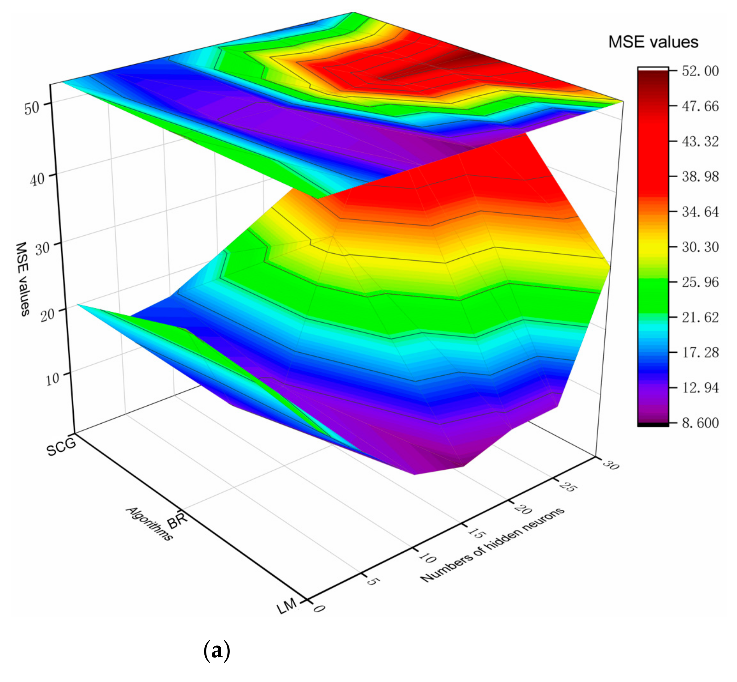
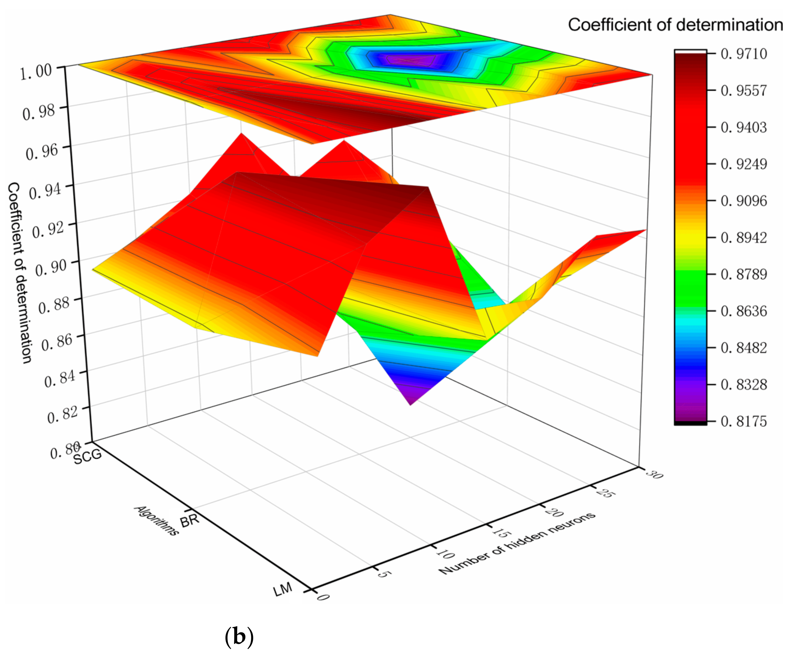
2.3.4. Performance Evaluation of ANN Architectures

In this study, customised combinations of different hidden neurons (1, 5, 10, 15, 20, 25, 30), hidden layers (1–2) and LM, BR and SCG algorithms have been employed. Furthermore, each pattern of ANN architectures has been trained for five times to improve the accuracy of models. In order to investigate the performance of the trained models in this study, two statistical analyses named MSE and $R^2$ are employed. MSE is the average value of the cost function for minimising the sum of squared errors (SSE) during the linear regression model fitting process. This represents the mean square error between the predicted and the actual value. MSE value is calculated according to Equation (8) [68]. The lower MSE value indicates a trained model with higher accuracy.

$$MSE=\frac{1}{n}{\displaystyle \sum }_{i=1}^n{(y{\prime }_i-y_i)}^2$$

(8)

where $n$ is the number of samples, and ($y{\prime }_i-y_i)$ is the result of the experimental value minus the predicted value on the testing sets being processed.

Moreover, $R^2$ value is employed as an assistance method to determine the performance of trained models defined in Equation (9).$R^2$ value exhibits the percentage of real value changes, which can be influenced by the variation of the predicted value. The range of $R^2$ value is from zero to one. Considering Equation (9), the numerator part represents the sum of the squared difference between the real value and the predicted value, similar to MSE. The denominator part represents the sum of the squared difference between the real value and the mean [70]. If the result is 0, it means that the model fits poorly. If the result is 1, it means that the model is error-free. Generally, the larger the $R^2$ value is, the better the model fitting effect is.

$$R^2=1-\frac{{{\displaystyle \sum }}_{i=1}^n{\left(y{\prime }_i-y_i\right)}^2}{{{\displaystyle \sum }}_{i=1}^n {\left(y_i-\overline{y}\right)}^2}$$

(9)

According to the aforementioned sections, the main steps to attain the optimum ANN architecture selection are demonstrated in Figure 2.

3. Results and Discussion

3.1. Optimum ANN Architecture Determination

The optimal ANN architecture is confirmed by embarking on the ANN architecture selection steps mentioned in the previous section. The MSE and R² values of the testing sets are defined as the performance evaluation index of all ANN architectures with 1–2 hidden layers and 1–30 hidden neurons, which are listed in

Table A1. MSE and R² value of all ANN architectures.

Training Group	ANN Architecture	MSE Value	Average Value	R2 Value	Average Value
LM-17-1-5	LM-17-1-5-1	19.608	23.1850	0.915	0.9026
	LM-17-1-5-2	27.179		0.889
	LM-17-1-5-3	23.363		0.906
	LM-17-1-5-4	20.507		0.907
	LM-17-1-5-5	25.268		0.895
BR-17-1-5	BR-17-1-5-1	24.124	26.4407	0.908	0.8955
	BR-17-1-5-2	27.455		0.889
	BR-17-1-5-3	26.468		0.889
	BR-17-1-5-4	24.760		0.896
	BR-17-1-5-5	29.395		0.895
SCG-17-1-5	SCG-17-1-5-1	28.627	20.1789	0.880	0.9166
	SCG-17-1-5-2	28.075		0.882
	SCG-17-1-5-3	13.612		0.946
	SCG-17-1-5-4	13.645		0.944
	SCG-17-1-5-5	16.935		0.930
LM-17-5-5	LM-17-5-5-1	45.467	17.7134	0.816	0.9281
	LM-17-5-5-2	15.738		0.937
	LM-17-5-5-3	9.336		0.961
	LM-17-5-5-4	7.743		0.973
	LM-17-5-5-5	10.283		0.953
BR-17-5-5	BR-17-5-5-1	13.150	12.7931	0.932	0.9437
	BR-17-5-5-2	11.543		0.955
	BR-17-5-5-3	11.961		0.950
	BR-17-5-5-4	16.931		0.931
	BR-17-5-5-5	10.381		0.950
SCG-17-5-5	SCG-17-5-5-1	16.181	15.3224	0.927	0.9289
	SCG-17-5-5-2	14.924		0.935
	SCG-17-5-5-3	14.129		0.938
	SCG-17-5-5-4	16.267		0.918
	SCG-17-5-5-5	15.111		0.926
LM-17-10-5	LM-17-10-5-1	6.384	10.9459	0.973	0.9560
	LM-17-10-5-2	12.171		0.948
	LM-17-10-5-3	8.397		0.964
	LM-17-10-5-4	17.776		0.933
	LM-17-10-5-5	10.002		0.963
BR-17-10-5	BR-17-10-5-1	10.045	12.5805	0.956	0.9479
	BR-17-10-5-2	12.745		0.946
	BR-17-10-5-3	12.889		0.947
	BR-17-10-5-4	12.937		0.945
	BR-17-10-5-5	14.286		0.946
SCG-17-10-5	SCG-17-10-5-1	14.474	16.4983	0.940	0.9317
	SCG-17-10-5-2	20.373		0.915
	SCG-17-10-5-3	15.608		0.944
	SCG-17-10-5-4	13.072		0.945
	SCG-17-10-5-5	18.964		0.914
LM-17-15-5	LM-17-15-5-1	9.135	8.7459	0.965	0.9626
	LM-17-15-5-2	9.664		0.958
	LM-17-15-5-3	10.259		0.952
	LM-17-15-5-4	6.710		0.973
	LM-17-15-5-5	7.961		0.965
BR-17-15-5	BR-17-15-5-1	20.356	32.3697	0.919	0.8795
	BR-17-15-5-2	40.857		0.861
	BR-17-15-5-3	22.650		0.920
	BR-17-15-5-4	40.554		0.858
	BR-17-15-5-5	37.433		0.839
SCG-17-15-5	SCG-17-15-5-1	14.682	20.5665	0.946	0.9146
	SCG-17-15-5-2	21.556		0.910
	SCG-17-15-5-3	29.309		0.878
	SCG-17-15-5-4	13.980		0.936
	SCG-17-15-5-5	23.306		0.904
LM-17-20-5	LM-17-20-5-1	10.841	11.0165	0.954	0.9509
	LM-17-20-5-2	14.187		0.946
	LM-17-20-5-3	9.020		0.956
	LM-17-20-5-4	8.129		0.968
	LM-17-20-5-5	12.905		0.930
BR-17-20-5	BR-17-20-5-1	47.893	48.5124	0.840	0.8315
	BR-17-20-5-2	54.524		0.813
	BR-17-20-5-3	36.495		0.865
	BR-17-20-5-4	39.970		0.858
	BR-17-20-5-5	63.679		0.781
SCG-17-20-5	SCG-17-20-5-1	22.263	17.2641	0.915	0.9315
	SCG-17-20-5-2	13.949		0.946
	SCG-17-20-5-3	21.249		0.914
	SCG-17-20-5-4	17.420		0.935
	SCG-17-20-5-5	11.439		0.948
LM-17-25-5	LM-17-25-5-1	8.471	11.267	0.970	0.9522
	LM-17-25-5-2	10.370		0.957
	LM-17-25-5-3	14.410		0.931
	LM-17-25-5-4	10.994		0.950
	LM-17-25-5-5	12.090		0.953
BR-17-25-5	BR-17-25-5-1	69.336	49.6730	0.761	0.8305
	BR-17-25-5-2	59.611		0.811
	BR-17-25-5-3	43.495		0.846
	BR-17-25-5-4	35.384		0.864
	BR-17-25-5-5	40.540		0.870
SCG-17-25-5	SCG-17-25-5-1	11.784	15.9628	0.944	0.9271
	SCG-17-25-5-2	12.815		0.942
	SCG-17-25-5-3	18.111		0.910
	SCG-17-25-5-4	17.119		0.925
	SCG-17-25-5-5	19.986		0.914
LM-17-30-5	LM-17-30-5-1	20.039	29.3399	0.909	0.8847
	LM-17-30-5-2	24.060		0.904
	LM-17-30-5-3	29.875		0.871
	LM-17-30-5-4	36.002		0.855
	LM-17-30-5-5	36.724		0.884
BR-17-30-5	BR-17-30-5-1	50.004	51.8540	0.828	0.8298
	BR-17-30-5-2	54.383		0.819
	BR-17-30-5-3	44.388		0.882
	BR-17-30-5-4	52.017		0.824
	BR-17-30-5-5	58.478		0.796
CG-17-30-5	SCG-17-30-5-1	19.643	21.8357	0.916	0.9115
	SCG-17-30-5-2	20.886		0.904
	SCG-17-30-5-3	17.442		0.925
	SCG-17-30-5-4	23.130		0.919
	SCG-17-30-5-5	28.078		0.894
LM-17-1-1-5	LM-17-1-1-5-1	23.061	21.5373	0.897	0.9078
	LM-17-1-1-5-2	16.666		0.922
	LM-17-1-1-5-3	15.999		0.940
	LM-17-1-1-5-4	21.057		0.915
	LM-17-1-1-5-5	30.904		0.865
BR -17-1-1-5	BR-17-1-1-5-1	28.043	28.2334	0.895	0.8914
	BR-17-1-1-5-2	26.079		0.903
	BR-17-1-1-5-3	29.380		0.889
	BR-17-1-1-5-4	31.593		0.886
	BR-17-1-1-5-5	26.073		0.884
SCG -17-1-1-5	SCG-17-1-1-5-1	29.392	25.4727	0.884	0.8937
	SCG-17-1-1-5-2	22.598		0.892
	SCG-17-1-1-5-3	21.492		0.904
	SCG-17-1-1-5-4	26.143		0.896
	SCG-17-1-1-5-5	27.738		0.892
LM-17-5-5-5	LM-17-5-5-5-1	9.222	11.1077	0.958	0.9522
	LM-17-5-5-5-2	11.546		0.945
	LM-17-5-5-5-3	8.044		0.967
	LM-17-5-5-5-4	14.946		0.933
	LM-17-5-5-5-5	11.780		0.958
BR -17-5-5-5	BR-17-5-5-5-1	6.122	9.1582	0.980	0.9623
	BR-17-5-5-5-2	7.082		0.974
	BR-17-5-5-5-3	7.614		0.966
	BR-17-5-5-5-4	6.123		0.973
	BR-17-5-5-5-5	18.850		0.919
SCG -17-5-5-5	SCG-17-5-5-5-1	22.845	22.9340	0.912	0.9049
	SCG-17-5-5-5-2	21.129		0.910
	SCG-17-5-5-5-3	24.037		0.902
	SCG-17-5-5-5-4	22.576		0.905
	SCG-17-5-5-5-5	24.083		0.896
LM-17-10-10-5	LM-17-10-10-5-1	7.694	7.2420	0.970	0.9710
	LM-17-10-10-5-2	6.067		0.974
	LM-17-10-10-5-3	5.669		0.978
	LM-17-10-10-5-4	8.088		0.964
	LM-17-10-10-5-5	8.692		0.969
BR -17-10-10-5	BR-17-10-10-5-1	26.057	25.1978	0.906	0.9071
	BR-17-10-10-5-2	18.578		0.927
	BR-17-10-10-5-3	35.363		0.877
	BR-17-10-10-5-4	25.603		0.906
	BR-17-10-10-5-5	20.387		0.919
SCG -17-10-10-5	SCG-17-10-10-5-1	18.176	19.3592	0.934	0.9227
	SCG-17-10-10-5-2	22.484		0.930
	SCG-17-10-10-5-3	19.166		0.911
	SCG-17-10-10-5-4	18.794		0.916
	SCG-17-10-10-5-5	18.177		0.923
LM-17-15-15-5	LM-17-15-15-5-1	29.132	30.3840	0.892	0.8923
	LM-17-15-15-5-2	40.439		0.861
	LM-17-15-15-5-3	15.351		0.941
	LM-17-15-15-5-4	34.254		0.884
	LM-17-15-15-5-5	32.744		0.884
BR -17-15-15-5	BR-17-15-15-5-1	30.100	35.5664	0.908	0.8674
	BR-17-15-15-5-2	48.677		0.824
	BR-17-15-15-5-3	30.691		0.899
	BR-17-15-15-5-4	43.835		0.791
	BR-17-15-15-5-5	24.530		0.915
SCG -17-15-15-5	SCG-17-15-15-5-1	12.935	11.6450	0.942	0.9500
	SCG-17-15-15-5-2	11.981		0.951
	SCG-17-15-15-5-3	7.689		0.970
	SCG-17-15-15-5-4	12.935		0.940
	SCG-17-15-15-5-5	12.687		0.946
LM-17-20-20-5	LM-17-20-20-5-1	22.755	23.9056	0.903	0.9053
	LM-17-20-20-5-2	29.075		0.885
	LM-17-20-20-5-3	25.528		0.891
	LM-17-20-20-5-4	25.748		0.911
	LM-17-20-20-5-5	16.422		0.936
BR -17-20-20-5	BR-17-20-20-5-1	60.931	54.9310	0.795	0.8179
	BR-17-20-20-5-2	45.471		0.857
	BR-17-20-20-5-3	70.394		0.796
	BR-17-20-20-5-4	42.445		0.829
	BR-17-20-20-5-5	55.414		0.813
SCG -17-20-20-5	SCG-17-20-20-5-1	13.649	20.3014	0.939	0.9178
	SCG-17-20-20-5-2	24.836		0.900
	SCG-17-20-20-5-3	29.018		0.876
	SCG-17-20-20-5-4	16.613		0.935
	SCG-17-20-20-5-5	17.391		0.939
LM-17-25-25-5	LM-17-25-25-5-1	29.484	18.4144	0.899	0.9285
	LM-17-25-25-5-2	18.306		0.930
	LM-17-25-25-5-3	16.619		0.933
	LM-17-25-25-5-4	13.342		0.941
	LM-17-25-25-5-5	14.321		0.940
BR -17-25-25-5	BR-17-25-25-5-1	62.883	42.4919	0.768	0.8455
	BR-17-25-25-5-2	48.863		0.804
	BR-17-25-25-5-3	39.218		0.872
	BR-17-25-25-5-4	35.220		0.882
	BR-17-25-25-5-5	26.276		0.902
SCG -17-25-25-5	SCG-17-25-25-5-1	19.483	16.5416	0.926	0.9346
	SCG-17-25-25-5-2	13.245		0.943
	SCG-17-25-25-5-3	18.428		0.929
	SCG-17-25-25-5-4	14.322		0.947
	SCG-17-25-25-5-5	17.231		0.928
LM-17-30-30-5	LM-17-30-30-5-1	6.665	19.0260	0.975	0.9247
	LM-17-30-30-5-2	21.629		0.918
	LM-17-30-30-5-3	25.859		0.892
	LM-17-30-30-5-4	6.398		0.975
	LM-17-30-30-5-5	34.579		0.864
BR -17-30-30-5	BR-17-30-30-5-1	49.909	39.5577	0.823	0.8571
	BR-17-30-30-5-2	31.449		0.874
	BR-17-30-30-5-3	49.542		0.824
	BR-17-30-30-5-4	31.739		0.893
	BR-17-30-30-5-5	35.149		0.871
SCG -17-30-30-5	SCG-17-30-30-5-1	20.650	22.2361	0.908	0.9074
	SCG-17-30-30-5-2	18.320		0.921
	SCG-17-30-30-5-3	23.257		0.903
	SCG-17-30-30-5-4	15.679		0.935
	SCG-17-30-30-5-5	33.275		0.869

. For instance, the ANN architecture LM-17-1-1-5, can be explained as the architecture employing the LM algorithm consisting of 17 input elements, five output elements, and one hidden neuron in two hidden layers. Figure 3 and Figure 4 visually illustrate MSE and R² values of all ANN architectures, respectively. The MSE value of all ANN architectures with one hidden layer is demonstrated in Figure 3a. From Figure 3a, the MSE values of the ANN models with SCG algorithm fluctuate around 20 within 30 hidden neurons. Furthermore, the MSE values of the ANN with LM and BR algorithms moderately decrease from 26.4407 to 12.5805, and from 23.1850 to 8.7459 when the hidden neurons are modified from one to ten and one to fifteen, respectively, followed by a dramatic increase in the MSE value from 8.7459 to 29.3400, and from 12.5805 to 51.8540 within 30 neurons. Moreover, the MSE values of all ANN architectures with two hidden layers are demonstrated in Figure 3b. Based on Figure 3b, the MSE values of all ANN architectures with two hidden layers go through slight drops within the first 15 hidden neurons in general. Thereafter, the MSE value of the ANN models with LM, BR and SCG algorithms decreases from 21.5373 to 7.2420, 28.2334 to 9.1582 and 25.4727 to 11.6450 when the hidden neurons are changed from one to ten, one to five and one to fifteen, respectively. Subsequently, the MSE values of the ANN with LM and BR algorithms soar between 7.2420 and 30.3840, and between 9.1582 and 54.9310 from ten to fifteen hidden layers and five to twenty hidden layers, respectively. Meanwhile, the MSE value of the ANN model with SCG slightly increases from 11.6450 to 22.2361 between 15 and 30 hidden neurons. Afterwards, the MSE values of the ANN models with LM and BR algorithms moderately drop from 30.3840 to 19.0260, and from 54.9310 to 39.5577 when the hidden neurons are changed from 15 to 30, and from 20 to 30, respectively. It can be concluded that the minimum MSE values of ANN architectures with one and two hidden layers are 8.7459 and 7.2420 derived from LM-17-15-5 and LM-17-10-10-5, respectively. The increasing MSE values of ANN models with various architectures can be attributed to two problems: (i) the underfitting problem, and (ii) the overfitting problem. Considering the underfitting problem, the learning capacity of ANN models is relatively low because the numbers of the hidden layers or neurons of ANN models are rather insufficient to stimulate the complicated relationships between the inputs and the outputs, then resulting in a weak generalisation capacity of ANN models. On the contrary, the overfitting problem occurs when the learning capacity of ANN models is overly high. In other words, every single datum can be captured by ANN models. Thus, the MSE value of ANN models soars because the generalisation capacity of ANN models decreases owing to the overfitting problem.

With regard to Figure 4a,b, the trend of changes in R² value is observed to be the same as the MSE value shown in Figure 3a,b. The maximum R² value of ANN architectures with one hidden layer and two hidden layers are 0.9626 and 0.9710 at LM-17-15-5 and LM-17-10-10-5, respectively. It can be summarised that the ANN architecture with LM algorithm, which consists of two hidden layers with ten neurons in each layer, shows the lowest MSE value but the highest R² value of 7.2420 and 0.9710, respectively. Thus, the best ANN architecture for predicting multiple mechanical properties of rubberised concrete is LM-17-10-10-5.

The optimal ANN architecture for predicting multiple mechanical properties of rubberised concrete has been determined by utilising different algorithms (LM, BR and SCG), hidden layers (one and two layers) and hidden neurons (1, 5, 10, 15, 20, 25, 30) in this study. Each of the ANN architectures contains 17 inputs and five outputs. The comparison of each experimental and predicted mechanical property by employing the optimal ANN architecture, LM-17-10-10-5, is exhibited in Figure 5. The R² value indicates the capacity of ANN models for predicting each mechanical property of rubberised concrete. The line charts demonstrate the difference between the experimental and the predicted value. Regarding Figure 5a–d,i,j, the R² values of CS7, CS28 and EM are 0.9552, 0.9641 and 0.9576, respectively. The R² value of these mechanical properties is recognised as a high prediction accuracy. The R² value of the ANN model, which predicts FS, is 0.8493 that is relatively lower than that of the ANN models for predicting CS7, CS28 and EM. Moreover, the R² of the ANN model for predicting STS, 0.6545, is the lowest among all ANN models in this study. Based on Figure 5h, the fitting line cannot coincide completely with the Y = T line. Namely, there is a certain degree of deviation between the two lines. This phenomenon also can be found in Figure 5g. For instance, the predicted STS is 5.70 MPa and 4.54 MPa, which are significantly lower than the experimental STS of 8.00 MPa and 7.00 MPa at sample 256 and sample 225, respectively. This phenomenon can be attributed to the underfitting of the model. The ANN model is too simple to explain the relationship between the inputs and STS.

3.2. Comparative Analysis

In the previous section, the optimal ANN architecture has been selected as LM-17-10-10-5 by comparisons using the MSE and R² values. Linear regression has been commonly utilised to simulate the complicated relationship between the dependent and independent factors. To inspect the prediction accuracy of the optimal ANN architecture, MLR has been adopted in this study. Therefore, the prediction accuracy of both methods is defined by employing R². The higher the R² value, the better the prediction accuracy. The complicated relationship between 17 inputs and five outputs is calculated by employing MLR, explained in Equation (10) [30].

$$y=a_0+a_1{x}_1+a_2{x}_2+\dots +a_m{x}_m$$

(10)

where, $y$ indicates the predicted mechanical properties, $x_m$ denotes the independent variables, $a_0$ denotes the y-intercept, and $a_m$ indicates the regression coefficients. The regression coefficients are similar to the traditional regression models by applying the least square method shown in Equation (10). Therefore, the best function can be identified by minimising the sum of squared errors between experimental and predicted values. MLR has been conducted by employing “SPSS Statistics R27” in this study. The data sets are split at a ratio 8:2 for training and testing. The R² value of each predicted mechanical property derived from MLR and the optimal ANN model are demonstrated in

Table 7. R² value of multiple linear regression (MLR) and the ANN model.

Predicted Mechanical Properties	MLR	ANN (LM-17-10-10-5)
CS7	0.660	0.9552
CS28	0.673	0.9641
FS	0.601	0.8493
STS	0.460	0.6545
EM	0.773	0.9576

. According to Table 7, the R² values of MLR for predicting the CS7, CS28, FS, STS and EM of rubberised concrete are 0.660, 0.673, 0.601, 0.460 and 0.773, respectively. It is evident that the R² value of MLR is relatively lower than that of the optimal ANN model. It can be interpreted that the prediction accuracy of MLR for predicting mechanical properties of rubberised concrete is lower than that of the ANN models. Wherein, the attention should be paid to STS prediction of MLR. Note that the R² value of MLR for STS prediction (around 0.460) is much lower than those of the other prediction models for mechanical properties. The reason can be attributed to the fact that the relationship between the inputs and the tensile strength is nonlinear. Of interest, the same phenomenon occurs when STS is predicted by employing ANN models.

4. Conclusions

This study is the world’s first to establish a novel machine learning-aided design and prediction of eco-friendly rubberised concrete, enhancing engineering applications for sustainable infrastructures towards net-zero emission. The advanced machine learning approach is capable of designing and predcting multiple attributes (i.e., mechanical properties) simultaneously, which is a key novelty of this study. This approach is more rational and practical since, in reality, engineers need to satisfy all limit states criteria (for both serviceability and ultimate conditions). To enable the study, a comprehensive collection of 353 data sets consisting of 17 input elements of pertinent rubberised concrete including its five mechanical properties as outputs have been collected from all reputable sources in the open literature, and have been processed for training and testing a variety of ANN models. ANN models with 1–2 hidden layers, 1–30 hidden neurons and three types of algorithms (LM, BR and SCG) have been designed, validated and evaluated by benchmarking the $R^2$ values and MSE values. Subsequently, the optimal ANN architecture, which best predicts the outcome, has been customised and obtained as LM-17-10-10-5. Then, the $R^2$ value acting as the prediction accuracy index of MLR was compared with that of the optimal ANN model. The conclusions can be drawn as follows:

• The ANN architecture with LM algorithm, two hidden layers and ten hidden neurons in each hidden layer is the optimal option for simultaneously predicting multiple mechanical properties of eco-friendly rubberised concrete.
• Based on the MSE (7.2420) and $R^2$ (0.9710) values of the optimal ANN architecture, excellent prediction accuracy of the machine learning can be attained.
• The $R^2$ value of MLR is relatively lower than that of the optimal ANN model. This traditionally implies that the prediction accuracy of the ANN model is relatively higher than that of MLR.

References

- Wright, B.; Garside, M.; Allgar, V.; Hodkinson, R.; Thorpe, H. A large population-based study of the mental health and wellbeing of children and young people in the North of England. Clin. Child Psychol. Psychiatry 2020, 25, 877–890. [Google Scholar] [CrossRef]
- Pacheco-Torgal, F.; Ding, Y.; Jalali, S. Properties and durability of concrete containing polymeric wastes (tyre rubber and polyethylene terephthalate bottles): An overview. Constr. Build. Mater. 2012, 30, 714–724. [Google Scholar] [CrossRef]
- Colom, X.; Carrillo, F.; Canavate, J. Composites reinforced with reused tyres: Surface oxidant treatment to improve the interfacial compatibility. Compos. Part A Appl. Sci. Manuf. 2007, 38, 44–50. [Google Scholar] [CrossRef]
- Toutanji, H.A. The use of rubber tire particles in concrete to replace mineral aggregates. Cem. Concr. Compos. 1996, 18, 135–139. [Google Scholar] [CrossRef]
- Shu, X.; Huang, B. Recycling of waste tire rubber in asphalt and portland cement concrete: An overview. Constr. Build. Mater. 2014, 67, 217–224. [Google Scholar] [CrossRef]
- Alam, I.; Mahmood, U.A.; Khattak, N. Use of rubber as aggregate in concrete: A review. Int. J. Adv. Struct. Geotech. Eng. 2015, 4, 92–96. [Google Scholar]
- Kaewunruen, S.; Ngamkhanong, C.; Lim, C.H. Damage and failure modes of railway prestressed concrete sleepers with holes/web openings subject to impact loading conditions. Eng. Struct. 2018, 176, 840–848. [Google Scholar] [CrossRef]
- Rashad, A.M. A comprehensive overview about recycling rubber as fine aggregate replacement in traditional cementitious materials. Int. J. Sustain. Built Environ. 2016, 5, 46–82. [Google Scholar] [CrossRef]
- Sukontasukkul, P. Use of crumb rubber to improve thermal and sound properties of pre-cast concrete panel. Constr. Build. Mater. 2009, 23, 1084–1092. [Google Scholar] [CrossRef]
- You, R.; Goto, K.; Ngamkhanong, C.; Kaewunruen, S. Nonlinear finite element analysis for structural capacity of railway prestressed concrete sleepers with rail seat abrasion. Eng. Fail. Anal. 2019, 95, 47–65. [Google Scholar] [CrossRef]
- Thomas, B.S.; Kumar, S.; Mehra, P.; Gupta, R.C.; Joseph, M.; Csetenyi, L.J. Abrasion resistance of sustainable green concrete containing waste tire rubber particles. Constr. Build. Mater. 2016, 124, 906–909. [Google Scholar] [CrossRef]
- Benazzouk, A.; Mezreb, K.; Doyen, G.; Goullieux, A.; Quéneudec, M. Effect of rubber aggregates on the physico-mechanical behaviour of cement–rubber composites-influence of the alveolar texture of rubber aggregates. Cem. Concr. Compos. 2003, 25, 711–720. [Google Scholar] [CrossRef]
- Thomas, B.S.; Gupta, R.C. Long term behaviour of cement concrete containing discarded tire rubber. J. Clean. Prod. 2015, 102, 78–87. [Google Scholar] [CrossRef]
- Eldin, N.N.; Senouci, A.B. Rubber-tire particles as concrete aggregate. J. Mater. Civ. Eng. 1993, 5, 478–496. [Google Scholar] [CrossRef]
- Roychand, R.; Gravina, R.J.; Zhuge, Y.; Ma, X.; Youssf, O.; Mills, J.E. A comprehensive review on the mechanical properties of waste tire rubber concrete. Constr. Build. Mater. 2020, 237, 117651. [Google Scholar] [CrossRef]
- Youssf, O.; Mills, J.E.; Benn, T.; Zhuge, Y.; Ma, X.; Roychand, R.; Gravina, R. Development of Crumb Rubber Concrete for Practical Application in the Residential Construction Sector–Design and Processing. Constr. Build. Mater. 2020, 260, 119813. [Google Scholar] [CrossRef]
- Wu, Y.-F.; Kazmi, S.M.S.; Munir, M.J.; Zhou, Y.; Xing, F. Effect of compression casting method on the compressive strength, elastic modulus and microstructure of rubber concrete. J. Clean. Prod. 2020, 264, 121746. [Google Scholar] [CrossRef]
- Kazmi, S.M.S.; Munir, M.J.; Wu, Y.-F. Application of waste tire rubber and recycled aggregates in concrete products: A new compression casting approach. Resour. Conserv. Recycl. 2021, 167, 105353. [Google Scholar] [CrossRef]
- Vieira, S.; Gong, Q.-Y.; Pinaya, W.H.; Scarpazza, C.; Tognin, S.; Crespo-Facorro, B.; Tordesillas-Gutierrez, D.; Ortiz-García, V.; Setien-Suero, E.; Scheepers, F.E. Using machine learning and structural neuroimaging to detect first episode psychosis: Reconsidering the evidence. Schizophr. Bull. 2020, 46, 17–26. [Google Scholar] [CrossRef]
- Michie, D.; Spiegelhalter, D.J.; Taylor, C. Machine learning. Neural Stat. Classif. 1994, 13, 1–298. [Google Scholar]
- Goodfellow, I.; Bengio, Y.; Courville, A.; Bengio, Y. Deep Learning; MIT Press: Cambridge, UK, 2016; Volume 1. [Google Scholar]
- Goharzay, M.; Noorzad, A.; Ardakani, A.M.; Jalal, M. Computer-aided SPT-based reliability model for probability of liquefaction using hybrid PSO and GA. J. Comput. Des. Eng. 2020, 7, 107–127. [Google Scholar] [CrossRef]
- Chaabene, W.B.; Flah, M.; Nehdi, M.L. Machine learning prediction of mechanical properties of concrete: Critical review. Constr. Build. Mater. 2020, 260, 119889. [Google Scholar] [CrossRef]
- Dantas, A.T.A.; Leite, M.B.; de Jesus Nagahama, K. Prediction of compressive strength of concrete containing construction and demolition waste using artificial neural networks. Constr. Build. Mater. 2013, 38, 717–722. [Google Scholar] [CrossRef]
- Behnood, A.; Golafshani, E.M. Predicting the compressive strength of silica fume concrete using hybrid artificial neural network with multi-objective grey wolves. J. Clean. Prod. 2018, 202, 54–64. [Google Scholar] [CrossRef]
- Erdal, H.I.; Karakurt, O.; Namli, E. High performance concrete compressive strength forecasting using ensemble models based on discrete wavelet transform. Eng. Appl. Artif. Intell. 2013, 26, 1246–1254. [Google Scholar] [CrossRef]
- Tanarslan, H.; Secer, M.; Kumanlioglu, A. An approach for estimating the capacity of RC beams strengthened in shear with FRP reinforcements using artificial neural networks. Constr. Build. Mater. 2012, 30, 556–568. [Google Scholar] [CrossRef]
- Barbuta, M.; Diaconescu, R.-M.; Harja, M. Using neural networks for prediction of properties of polymer concrete with fly ash. J. Mater. Civ. Eng. 2012, 24, 523–528. [Google Scholar] [CrossRef]
- Gencel, O.; Kocabas, F.; Gok, M.S.; Koksal, F. Comparison of artificial neural networks and general linear model approaches for the analysis of abrasive wear of concrete. Constr. Build. Mater. 2011, 25, 3486–3494. [Google Scholar] [CrossRef]
- Yoon, J.Y.; Kim, H.; Lee, Y.-J.; Sim, S.-H. Prediction model for mechanical properties of lightweight aggregate concrete using artificial neural network. Materials 2019, 12, 2678. [Google Scholar] [CrossRef]
- Khademi, F.; Jamal, S.M.; Deshpande, N.; Londhe, S. Predicting strength of recycled aggregate concrete using artificial neural network, adaptive neuro-fuzzy inference system and multiple linear regression. Int. J. Sustain. Built Environ. 2016, 5, 355–369. [Google Scholar] [CrossRef]
- Topçu, İ.B.; Sarıdemir, M. Prediction of mechanical properties of recycled aggregate concretes containing silica fume using artificial neural networks and fuzzy logic. Comput. Mater. Sci. 2008, 42, 74–82. [Google Scholar] [CrossRef]
- Grekousis, G. Artificial neural networks and deep learning in urban geography: A systematic review and meta-analysis. Comput. Environ. Urban Syst. 2019, 74, 244–256. [Google Scholar] [CrossRef]
- Liu, H.; Wang, X.; Jiao, Y.; Sha, T. Experimental investigation of the mechanical and durability properties of crumb rubber concrete. Materials 2016, 9, 172. [Google Scholar] [CrossRef]
- Hernández-Olivares, F.; Barluenga, G. Fire performance of recycled rubber-filled high-strength concrete. Cem. Concr. Res. 2004, 34, 109–117. [Google Scholar] [CrossRef]
- Kaewunruen, S.; Meesit, R. Eco-friendly High-Strength Concrete Engineered by Micro Crumb Rubber from Recycled Tires and Plastics for Railway Components. Adv. Civ. Eng. Mater. 2020, 9, 210–226. [Google Scholar] [CrossRef]
- Yung, W.H.; Yung, L.C.; Hua, L.H. A study of the durability properties of waste tire rubber applied to self-compacting concrete. Constr. Build. Mater. 2013, 41, 665–672. [Google Scholar] [CrossRef]
- Najim, K.B.; Hall, M.R. Mechanical and dynamic properties of self-compacting crumb rubber modified concrete. Constr. Build. Mater. 2012, 27, 521–530. [Google Scholar] [CrossRef]
- Choudhary, S.; Chaudhary, S.; Jain, A.; Gupta, R. Assessment of effect of rubber tyre fiber on functionally graded concrete. Mater. Today Proc. 2020, 28, 1496–1502. [Google Scholar] [CrossRef]
- Onuaguluchi, O.; Panesar, D.K. Hardened properties of concrete mixtures containing pre-coated crumb rubber and silica fume. J. Clean. Prod. 2014, 82, 125–131. [Google Scholar] [CrossRef]
- Xue, J.; Shinozuka, M. Rubberized concrete: A green structural material with enhanced energy-dissipation capability. Constr. Build. Mater. 2013, 42, 196–204. [Google Scholar] [CrossRef]
- Ganjian, E.; Khorami, M.; Maghsoudi, A.A. Scrap-tyre-rubber replacement for aggregate and filler in concrete. Constr. Build. Mater. 2009, 23, 1828–1836. [Google Scholar] [CrossRef]
- Kaewunruen, S.; Li, D.; Chen, Y.; Xiang, Z. Enhancement of Dynamic Damping in Eco-Friendly Railway Concrete Sleepers Using Waste-Tyre Crumb Rubber. Materials 2018, 11, 1169. [Google Scholar] [CrossRef]
- Liu, F.; Zheng, W.; Li, L.; Feng, W.; Ning, G. Mechanical and fatigue performance of rubber concrete. Constr. Build. Mater. 2013, 47, 711–719. [Google Scholar] [CrossRef]
- Issa, C.A.; Salem, G. Utilization of recycled crumb rubber as fine aggregates in concrete mix design. Constr. Build. Mater. 2013, 42, 48–52. [Google Scholar] [CrossRef]
- Sukontasukkul, P.; Tiamlom, K. Expansion under water and drying shrinkage of rubberised concrete mixed with crumb rubber with different size. Constr. Build. Mater. 2012, 29, 520–526. [Google Scholar] [CrossRef]
- Pelisser, F.; Zavarise, N.; Longo, T.A.; Bernardin, A.M. Concrete made with recycled tire rubber: Effect of alkaline activation and silica fume addition. J. Clean. Prod. 2011, 19, 757–763. [Google Scholar] [CrossRef]
- Khaloo, A.R.; Dehestani, M.; Rahmatabadi, P. Mechanical properties of concrete containing a high volume of tire–rubber particles. Waste Manag. 2008, 28, 2472–2482. [Google Scholar] [CrossRef] [PubMed]
- Balaha, M.; Badawy, A.; Hashish, M. Effect of Using Ground Waste Tire Rubber as Fine Aggregate on the Behaviour of Concrete Mixes. Indian J. Eng. Mater. Sci. 2007, 14, 6. [Google Scholar]
- Youssf, O.; ElGawady, M.A.; Mills, J.E.; Ma, X. An experimental investigation of crumb rubber concrete confined by fibre reinforced polymer tubes. Constr. Build. Mater. 2014, 53, 522–532. [Google Scholar] [CrossRef]
- Aiello, M.A.; Leuzzi, F. Waste tyre rubberised concrete: Properties at fresh and hardened state. Waste Manag. 2010, 30, 1696–1704. [Google Scholar] [CrossRef]
- Güneyisi, E.; Gesoğlu, M.; Özturan, T. Properties of rubberised concretes containing silica fume. Cem. Concr. Res. 2004, 34, 2309–2317. [Google Scholar] [CrossRef]
- Ling, T.-C. Prediction of density and compressive strength for rubberised concrete blocks. Constr. Build. Mater. 2011, 25, 4303–4306. [Google Scholar] [CrossRef]
- AbdelAleem, B.H.; Hassan, A.A. Development of self-consolidating rubberised concrete incorporating silica fume. Constr. Build. Mater. 2018, 161, 389–397. [Google Scholar] [CrossRef]
- Medina, N.F.; Flores-Medina, D.; Hernández-Olivares, F. Influence of fibers partially coated with rubber from tire recycling as aggregate on the acoustical properties of rubberised concrete. Constr. Build. Mater. 2016, 129, 25–36. [Google Scholar] [CrossRef]
- Hilal, N.N. Hardened properties of self-compacting concrete with different crumb rubber size and content. Int. J. Sustain. Built Environ. 2017, 6, 191–206. [Google Scholar] [CrossRef]
- Khalil, E.; Abd-Elmohsen, M.; Anwar, A.M. Impact resistance of rubberised self-compacting concrete. Water Sci. 2015, 29, 45–53. [Google Scholar] [CrossRef]
- Gerges, N.N.; Issa, C.A.; Fawaz, S.A. Rubber concrete: Mechanical and dynamical properties. Case Stud. Constr. Mater. 2018, 9, e00184. [Google Scholar] [CrossRef]
- Bisht, K.; Ramana, P. Evaluation of mechanical and durability properties of crumb rubber concrete. Constr. Build. Mater. 2017, 155, 811–817. [Google Scholar] [CrossRef]
- Gupta, T.; Chaudhary, S.; Sharma, R.K. Mechanical and durability properties of waste rubber fiber concrete with and without silica fume. J. Clean. Prod. 2016, 112, 702–711. [Google Scholar] [CrossRef]
- Naderpour, H.; Rafiean, A.H.; Fakharian, P. Compressive strength prediction of environmentally friendly concrete using artificial neural networks. J. Build. Eng. 2018, 16, 213–219. [Google Scholar] [CrossRef]
- Dogan, E.; Ates, A.; Yilmaz, E.C.; Eren, B. Application of artificial neural networks to estimate wastewater treatment plant inlet biochemical oxygen demand. Environ. Prog. 2008, 27, 439–446. [Google Scholar] [CrossRef]
- Heaton, J. Introduction to the Math of Neural Networks (Beta-1); Heaton Research, Inc.: Chesterfield, MO, USA, 2011. [Google Scholar]
- Brownlee, J. Deep Learning for Time Series Forecasting: Predict the Future with MLPs, CNNs and LSTMs in Python; Machine Learning Mastery: Vermont, Australia, 2018. [Google Scholar]
- Tamura, S.I.; Tateishi, M. Capabilities of a four-layered feedforward neural network: Four layers versus three. IEEE Trans. Neural Netw. 1997, 8, 251–255. [Google Scholar] [CrossRef] [PubMed]
- Li, J.-Y.; Chow, T.W.; Yu, Y.-L. The estimation theory and optimisation algorithm for the number of hidden units in the higher-order feedforward neural network. In Proceedings of the ICNN’95-International Conference on Neural Networks, Perth, WA, Australia, 27 November–1 December 1995; pp. 1229–1233. [Google Scholar]
- Sheela, K.G.; Deepa, S.N. Review on methods to fix number of hidden neurons in neural networks. Math. Probl. Eng. 2013, 2013. [Google Scholar] [CrossRef]
- Atici, U. Prediction of the strength of mineral admixture concrete using multivariable regression analysis and an artificial neural network. Expert Syst. Appl. 2011, 38, 9609–9618. [Google Scholar] [CrossRef]
- Duan, Z.-H.; Kou, S.-C.; Poon, C.-S. Using artificial neural networks for predicting the elastic modulus of recycled aggregate concrete. Constr. Build. Mater. 2013, 44, 524–532. [Google Scholar] [CrossRef]
- Bilim, C.; Atiş, C.D.; Tanyildizi, H.; Karahan, O. Predicting the compressive strength of ground granulated blast furnace slag concrete using artificial neural network. Adv. Eng. Softw. 2009, 40, 334–340. [Google Scholar] [CrossRef]
- Chou, J.-S.; Chiu, C.-K.; Farfoura, M.; Al-Taharwa, I. Optimising the prediction accuracy of concrete compressive strength based on a comparison of data-mining techniques. J. Comput. Civ. Eng. 2011, 25, 242–253. [Google Scholar] [CrossRef]
- Chithra, S.; Kumar, S.S.; Chinnaraju, K.; Ashmita, F.A. A comparative study on the compressive strength prediction models for High Performance Concrete containing nano silica and copper slag using regression analysis and Artificial Neural Networks. Constr. Build. Mater. 2016, 114, 528–535. [Google Scholar] [CrossRef]
- Dao, D.V.; Ly, H.-B.; Trinh, S.H.; Le, T.-T.; Pham, B.T. Artificial intelligence approaches for prediction of compressive strength of geopolymer concrete. Materials 2019, 12, 983. [Google Scholar] [CrossRef]
- Baghirli, O. Comparison of Lavenberg-Marquardt, Scaled Conjugate Gradient and Bayesian Regularisation Backpropagation Algorithms for Multistep Ahead Wind Speed Forecasting Using Multilayer Perceptron Feedforward Neural Network. Master’s Thesis, Uppsala University, Uppsala, Sweden, 2015. [Google Scholar]
- Levenberg, K. A method for the solution of certain nonlinear problems in least squares. Q. Appl. Math. 1944, 2, 164–168. [Google Scholar] [CrossRef]
- Marquardt, D.W. An algorithm for least-squares estimation of nonlinear parameters. J. Soc. Ind. Appl. Math. 1963, 11, 431–441. [Google Scholar] [CrossRef]
- Yue, Z.; Songzheng, Z.; Tianshi, L. Bayesian regularisation BP Neural Network model for predicting oil-gas drilling cost. In Proceedings of the 2011 International Conference on Business Management and Electronic Information, Guangzhou, China, 13–15 May 2011; pp. 483–487. [Google Scholar]
- Eren, B.; Yaqub, M.; Eyüpoğlu, V. Assessment of neural network training algorithms for the prediction of polymeric inclusion membranes efficiency. Sak. Üniversitesi Fen Bilimleri Enstitüsü Derg. 2016, 20, 533–542. [Google Scholar] [CrossRef][Green Version]
- Møller, M.F. A scaled conjugate gradient algorithm for fast supervised learning. Neural Netw. 1993, 6, 525–533. [Google Scholar] [CrossRef]
- Watrous, R.L. Learning Algorithms for Connectionist Networks: Applied Gradient Methods of Nonlinear Optimization; MIT Press: Cambridge, MA, USA, 1988. [Google Scholar]
- Kaewunruen, S.; Sussman, J.M.; Matsumoto, A. Grand challenges in transportation and transit systems. Front. Built Environ. 2016, 2. [Google Scholar] [CrossRef]