Air Pollution Assessment in China: A Novel Group Multiple Criteria Decision Making Model under Uncertain Information

Abstract

Assessment of and controlling air pollution are urgent global issues where international cooperation is deemed necessary. Although a very relevant data source can be obtained through continuous monitoring of air quality, measuring air pollutant concentrations is quite difficult when compared to other environmental indicators. We mainly have three different aims for the current study: (1) we propose the computation of the interval weights of decision makers (DMs) based on a group multiple criteria decision making (GMCDM) model; (2) we aim to rank the overall preferences of DMs by the possibility concepts; (3) we aim to evaluate the air quality in China using the most recent data based on our proposed method. We consider three monitoring stations, namely Luhu Park, Wanqingsha, and Tianhu, and the data for SO${}_2$, NO${}_2$, and PM${}_{10}$ are collected for November 2017, 2018, and 2019. The results from our innovative model show that November 2019 had the best air quality. Finally, robustness analyses are also performed to confirm the discriminatory power of the proposed approach.

1. Introduction

The industrial revolution was the trigger for the discharge of harmful substances into the air at a growing rate, which has been non-stop since 1850. Pollutant sources are now spread through industries and vehicles and increase from population increase and intense urbanization. As regards industries, thermal power plants, cement and steel works, refineries, the petrochemical industry, and mines are the most relevant sources of pollutants [1]. The negative externalities of air pollution are mostly related to health problems and environmental hazards; in this last case, the thinning of the atmospheric ozone layer gives rise to a vicious cycle of global warming and unpredictable climate consequences in a feedback process. The pollutants can be carried from one place to another through aerial transport [2,3,4]. In fact, pesticides have been discovered in Antarctica.

Monitoring and modeling are considered key tools for the environmental assessment of air pollution impacts, not only in terms of damage caused, but also in terms of future prospects, acting as a detection system and helping in evaluating and forecasting the environmental states. However, producing accurate measurements of air pollutant concentrations, when compared to other environmental elements, is quite difficult. Atmospheric dynamics cause its constituents to spread out geographically, very often resulting in a universal water and soil exposure for large populations without a chance for isolation. An additional issue is related to the fact that air pollution has a low level of concentration and that it interacts with other gases. In fact, many factors affect air quality and change with time. Broadly speaking, the interaction of multiple factors in the atmosphere leads to air pollution. It is possible to evaluate air pollution or air quality as an issue of a multiple criteria decision making (MCDM), which contains several contradictory or countervailing indicators including various air pollutants, the air quality index (AQI), and gross domestic product (GDP) per capita [5].

China is facing a number of issues that have a significant impact on both its short-term and long-term development. Air pollution will not only affect the country’s development in the long run, but it also has a significant negative influence on people’s lives in the short run from the perspective of the spread of different diseases [6]. World bank statistics show, regarding the mortality rate attributed to household and ambient air pollution, that in 2016, per 100,000 population, 112.7 people in China died because of air pollution, compared to the significantly lower numbers from the U.K., Germany, France, and Italy, where the numbers were 13.8, 16, 9.7, and 15, respectively.

Sulfur dioxide (SO${}_2$), is one of the key pollutants and contributors to death from air pollution globally, and it mainly results from power plants burning fossil fuels such as oil and gas, while other sources include metal smelters and volcanoes. Ships and other vehicles that burn sulfur also release SO${}_2$. Based on the data provided by the Euronews report [7], in 2018, China was the third ranked country in the world with SO${}_2$ emission reaching 2578 thousand tons, just following India and Russia. Nitrogen dioxide (NO${}_2$), is another air pollutant derived from road traffic and other fuel combustion. NO${}_2$ interacts with water, oxygen, and other chemicals in the atmosphere to form acid rain, which has a negative influence on the natural environment such as lakes and forest. In addition, breathing air with NO${}_2$ can irritate the airways in the human respiratory system, which eventually will lead to coughing, wheezing, or difficulty breathing. According to the data provided by the World Bank, China was the first ranked country with the largest amount of NO${}_2$ emissions as of 2012. According to earthobservatory.nasa.gov, over the period 2015–2019, 30–40 days after the lunar new year, the mean NO${}_2$ density in China reached around or even more than 250,000 umol/m${}^2$.

Besides SO${}_2$ and NO${}_2$, PM${}_{2.5}$, and PM${}_{10}$, denoting air particles with dynamic diameters less than 2.5 m and 10 m, respectively, are also important air pollutant in China [8]. The concentration of PM${}_{2.5}$ in Beijing was higher than the health standard set by the World Health Organization in 2013 [9], while at a more comprehensive level for 74 major cities in China over the period in 2013 and 2015, the average PM${}_{2.5}$ concentration was five-times higher than the health standard set by the World Health Organization [10]. In order to deal with this issue, the Chinese government not only formulated policies to regulate and control the emissions, but pollution abatement targets were set for different provinces and cities based on their own situation. Large efforts have been made by the Chinese government to encourage the use of clean energy both in industrial production and in the rural areas of China [11]. In addition to the effort to reduce emissions, the air quality monitoring and network construction have been strengthened by the Chinese government, which serve the purpose of studying the space–time features of air pollution in the country [12]. One observation from the research on air pollution in China is that most of the studies focused on the investigation of PM${}_{2.5}$; the examination of other pollutants such as SO${}_2$ and NO${}_2$ has not received enough attention from academic scholars [13].

MCDM problems may arise in different contexts, such as the automobile industry, construction engineering, manufacturing systems, economic evaluation, medical treatment, strategic planning, and environmental planning, among others [14,15,16,17,18]. Moreover, the ability of a single DM to assess all important perspectives and nuances of a problem in a comprehensive manner is limited by the inherent complexity of such socioeconomic contexts. As a matter of fact, compared to a single DM, a group of DMs generates additional complexities in the analysis. Typically, GMCDM relies on inviting a mix of internal and external experts to evaluate each air pollution criterion of every alternative geographical location on an individual basis. In light of the overall decision, the result is impacted by each DM in a different manner by means of their own weights or preferences with respect to each criterion. Determining DM weights is a crucial step in assuring an accurate and unbiased overall preference rank.

As regards the methods developed for GMCDM, French [19] used influence relations, which may exist among DMs, to determine the relative importance of a certain criterion in light of overall group members. On the other hand, Theil [20] designed a method based on correlation concepts should the DM inefficacy be measurable. In turn, Keeney and Kirkwood [21] advised in favor of using inter-personal comparisons to determine the weighted additive preference function. Ramanathan and Ganesh [22] proposed an intuitively simple eigenvector-based approach in which group members’ weights can be extracted according to their own preferences. Martel and Ben Khelifa [23] used individual outranking indices to address the GMCDM problem. The deviation measures, in which the additive linguistic preference relations were addressed to determine the DMs weight, were developed by Xu [24]. Chen and Fan [25] proposed factor scores to rank DM preferences.

In this paper, and different from previous research, we build upon the projection method designed by Xu [26] to compute the DM weights while ranking the alternatives based on straightforward and practical computations. It is worth noting that most of the previously mentioned research works relied on individual DM information structured as multiplicative preference matrices. Given that the determination of the exact criterion weights can become a cumbersome task, the use of weight intervals constitutes a flexible approach to overcome this issue [27].

Putting these methodologies into perspective, the use of MCDM models for measuring and monitoring air quality is a growing research field with a handful of recently published papers [28]. While MCDM methods have already been employed in air pollution measurement, the contribution of this research relies on the interval weight computation for each DM. To the best of our knowledge, this is the first time that a GMCDM model observing these features has been presented. In this paper, we dig further into computing the interval weights of DMs based on the projection method. Furthermore, and distinct from previous research, possibility fuzzy concepts are employed to rank the overall preferences of DMs. To further clarify, we mainly have three different aims for the current study: (1) we propose the computation of the interval weights of DMs based on a GMCDM model; (2) we aim to rank the overall preferences of DMs by the possibility concepts; (3) we aim to evaluate the air quality in China using the most recent data based on our proposed method.

This paper is structured as follows: The following section provides a literature review on the assessment of air pollution in China. Section 3 revisits the nonnegative interval number concept, offering computational and projection rules. Section 4 is devoted to presenting the novel GMCDM model designed for this research. Section 5 presents an application to different regions of the Pearl River in China, while the conclusion is provided in Section 6.

2. Literature Review

The issue related to the assessment of air pollution/air quality has been widely engaged by empirical researchers for different geographical locations, and various approaches have been used to investigate this topic including land use regression modeling and mobile monitoring [29,30,31], statistical analysis [32], multivariate analysis (including hierarchical agglomerate cluster analysis, principal component analysis, and multiple linear regression) [33,34], the proposed use of the air quality index [35], and the atmosphere evaluation and research integrated model [36].

The above-mentioned studies focused on countries/regions outside of China, while attempts have been widely made to evaluate the air pollution/quality in China. The air pollution index was proposed and used by Wang et al. [37] to assess the urban air quality of 86 cities in China over the period 2001–2011. The findings suggested that although Chinese cities have suffered the most from PM${}_{10}$, the air pollution index over this period declined from 7% to 1%, while the PM${}_{10}$ concentrations also experienced a consistent decrease. The proposal of the air pollution index should include more comprehensive pollution in the calculation, which is a limitation of this method and an area of future studies. Li et al. (2014) also conducted a similar study for Guangzhou, China, over the period 2001–2011. The results showed that the air pollution index is significantly and negatively affected by temperature, relative humidity, precipitation, and wind speed, while it is positively affected by diurnal temperature and atmospheric pressure.

Not only did researchers focus on the evaluation of air quality in China, but the empirical studies tried also to link the air pollution to other economic aspects such as energy consumption and economic development. In order to achieve this, the resource and environmental performance index was proposed by Gao et al. [38] between 2000 and 2012. The findings show that economic development affects energy consumption and air environment, but the influence was not shown to be significantly negative. The authors further argued that a positive impact of economic development on energy consumption and air pollution reduction can be achieved by optimizing the energy and industrial structure, improving energy efficiency, and formulating strict environmental policies.

A number of studies have also assessed the influence of air pollution on the mortality burden [39]. The log-linear exposure-response function was adopted for the former, and the integrated exposure response model was employed for the latter. Finally, the findings suggest that the mortality level is influenced by air pollution by different degrees across various areas in China. A multi-scale air quality modeling system was used by Gu and Yim [40] to stimulate air quality in China and to further study concentration-response functions. Not only is this study different from the previous two from the methodology perspective, but it is distinct in that it also focused on domestic trans-boundary pollutants and their impact on mortality. The results showed that 18% of premature mortalities from air pollution are attributed to the trans-boundary impact. The study further reported that 22% of mortalities in Taiwan were because of the trans-boundary impact from mainland China.

The linkage between air pollution and daily mortality in 16 Chinese cities over the period 1996 to 2018 was investigated by Chen et al. [41]. A tapered element oscillating microbalance is used to measure the concentration of PM${}_{10}$, while ultraviolet fluorescence and chemiluminescence were employed to measure the concentration of sulfur dioxide and nitrogen dioxide. In the second stage, two-stage Bayesian hierarchical statistical models were applied to assess the linkage between air pollution and daily mortality. The findings suggested that the mortality risk is significantly affected by short-term exposure to PM${}_{10}$. It further reported that certain groups of people, including females, older people, and less educated people, are more vulnerable to PM${}_{10}$.

An interesting piece of research was conducted by Sueyoshi and Yuan [42] to assess the regional performance in China over the period 2005–2012 under the non-parametric data envelopment analysis. In the model, total population, investment for preventing industrial pollution, electricity consumption, and final consumption of people were included as inputs. From the environment perspective, four undesirable outputs were used: PM${}_{2.5}$, PM${}_{10}$, SO${}_2$, and NO${}_2$, Finally, the gross regional product was used as the desirable output. The results showed that the northwest region is the area to which more economic resources should be distributed. In addition, the cities located in this area (including Beijing, Tianjin, Shanghai, and Chongqing) should have enhanced regulations on energy consumption for environmental protection purposes.

3. Preliminaries

In this section, we provide some preliminaries for the next sections. For this purpose, first, we introduce the interval numbers along with their operational rules, and then, the projection method is given.

3.1. Interval Number

Definition 1.

A non-negative interval number is defined as α = [$\underline{\alpha }$, $\overline{\alpha }$ ] = { x| 0 <$\underline{\alpha }$≤ x ≤ $\overline{\alpha }$ }.

Definition 2.

Consider two interval numbers $\alpha =[\underline{\alpha },\overline{\alpha }]$ and $\beta =[\underline{\beta },\overline{\beta }]$, and let η be a non-negative real number, then:

(a) α = $\beta \iff \underline{\alpha }$ = $\underline{\beta }$ and $\overline{\alpha }=\overline{\beta }$;

(b) $\alpha +\beta =[\underline{\alpha }+\underline{\beta },\overline{\alpha }+\overline{\beta }]$;

(c) $\eta \alpha =[\eta \underline{\alpha },\eta \overline{\alpha }]$.

Definition 3.

Suppose $A=\left\{{\alpha }_i\right|{\alpha }_i=[{\underline{\alpha }}_i,{\overline{\alpha }}_i],i=1,2,\dots ,k\}$. The weighted average operator of A is defined as:

$$WA{O}_A=\sum _{i=1}^k{w}_i{\alpha }_i$$

(1)

where $W={(w_1,w_2,\dots ,w_k)}^T$ is called the weight vector and ${\displaystyle \sum _{i=1}^k{w}_i=1}$.

Definition 4.

Let α and β be the same as Definition 2 and $l_{\alpha }=\overline{\alpha }-\underline{\alpha }$ and $l_{\beta }=\overline{\beta }-\underline{\beta }$ show respectively the length of α and β. We define the degree of possibility as [43].

$$P(\alpha \ge \beta )=max\{1-max(\frac{\overline{\beta }-\underline{\alpha }}{l_{\alpha }+l_{\beta }},0),0\}$$

(2)

Now, we propose a method to rank the interval arguments. In the proposed method, first using Equation (2), each ${\alpha }_i=[{\underline{\alpha }}_i,{\overline{\alpha }}_i]$ is compared with other ${\alpha }_j=[{\underline{\alpha }}_j,{\overline{\alpha }}_j],j=1,2,\dots ,n,$ and we assume $p_{ij}=p({\alpha }_i\ge {\alpha }_j)$. Then, we construct the matrix P as below:

$$P={\left[p_{ij}\right]}_{n\times n}$$

(3)

in which $p_{ij}\ge 0$ for all $i,j$.

Next, we sum up all the components in each row of P; that is,

$$p_i=\sum _{j=1}^n{p}_{ij},i=1,2,\dots ,n$$

(4)

Finally, using the $p_i,i=1,2,\dots ,n,$ values, the interval numbers ${\alpha }_i=[{\underline{\alpha }}_i,{\overline{\alpha }}_i],i=1,2,\dots ,n$ are ranked.

3.2. Projection Method

Definition 5.

Suppose ν is a vector such that $\nu =({\nu }_1,{\nu }_2,\dots ,{\nu }_n)$. Then, the module of ν is computed as:

$$\left|\nu \right|=\sqrt{\sum _{j=1}^n{\nu }_j^2}$$

(5)

Definition 6.

The inner product of two vectors $\nu =({\nu }_1,{\nu }_2,\dots ,{\nu }_n)$ and $\omega =({\omega }_1,{\omega }_2,\dots ,{\omega }_n)$ is calculated as:

$$\nu \omega =\sum _{j=1}^n{\nu }_j{\omega }_j$$

(6)

Definition 7.

Assume ν and ω are the same vectors as above. We define the projection of ν and ω by:

$$Pr{j}_{\omega }\left(\nu \right)=\left|\nu \right|cos(\nu ,\omega )=\left|\nu \right|\frac{\nu \omega }{\left|\nu \right|\left|\omega \right|}=\frac{\nu \omega }{\left|\omega \right|}$$

(7)

Figure 1 shows the projection of two vectors. Frankly speaking, the bigger $Pr{j}_{\omega }\left(\nu \right)$ represents that $\nu$ approaches with a greater degree to $\omega$. Using a similar method, the projection between the matrices is introduced.

Definition 8.

Let $A={\left[a_{ij}\right]}_{m\times n}$ and $B={\left[b_{ij}\right]}_{m\times n}$ be two matrices. We define the projection of A on B as below:

$$Pr{j}_B\left(A\right)=\frac{{\sum }_{i=1}^m{\sum }_{j=1}^n{a}_{ij}{b}_{ij}}{\sqrt{{\sum }_{i=1}^m{\sum }_{j=1}^n{b}_{ij}^2}}$$

(8)

4. Determining the Weights of DMs

Suppose there are m alternatives $A_1,A_2,\dots ,A_m$ and n attributes $u_1,u_2,\dots ,u_n$. Moreover, the weight vector of the attributes is denoted by $W={(w_1,w_2,\dots ,w_n)}^T$ such that $0\le w_j\le 1$ and ${\sum }_{j=1}^n{w}_j=1$, and there are t decision makers (DMs), $D_1,D_2,\dots ,D_t$, who construct the decision committee, and the weight vector of the DMs is denoted by $\lambda ={({\lambda }_1,{\lambda }_2,\dots ,{\lambda }_t)}^T$, where ${\lambda }_k\ge 0,{\sum }_{k=1}^n{\lambda }_k=1$. Let $M=\{1,2,\dots ,m\},N=\{1,2,\dots ,n\}$ and $T=\{1,2,\dots ,t\}$.

Now, we present an multiple attribute decision making (MADM) approach with uncertain information. The procedures of the proposed approach are described below.

Step 1. First construct the decision matrix for each DM, namely $D^{\left(K\right)},k=1,2,\dots ,t$.

$$D^k={\left([{\underline{x}}_{ij}^k,{\overline{x}}_{ij}^k]\right)}_{m\times n}=\begin{array}{cc}& \begin{array}{cccc}{u}_1\hspace{1em}\hspace{1em}& u_2\hspace{1em}\hspace{1em}& \cdots \hspace{1em} & u_n\end{array}\\ \begin{array}{l}{A}_1\\ A_2\\ ⋮\\ A_m\end{array}& \left(\begin{array}{cccc}[{\underline{x}}_{11}^k,{\overline{x}}_{11}^k]& [{\underline{x}}_{12}^k,{\overline{x}}_{12}^k]& \cdots & [{\underline{x}}_{1n}^k,{\overline{x}}_{1n}^k]\\ [{\underline{x}}_{21}^k,{\overline{x}}_{21}^k]& [{\underline{x}}_{22}^k,{\overline{x}}_{22}^k]& \cdots & [{\underline{x}}_{2n}^k,{\overline{x}}_{2n}^k]\\ ⋮& ⋮& \cdots & ⋮\\ [{\underline{x}}_{m1}^k,{\overline{x}}_{m1}^k]& [{\underline{x}}_{12}^k,{\overline{x}}_{12}^k]& \cdots & [{\underline{x}}_{mn}^k,{\overline{x}}_{mn}^k]\end{array}\right)\end{array}$$

(9)

Step 2. Use the following formulae to normalize the decision matrix.

$$R^k={([\frac{{\underline{x}}_{ij}^k}{max{\overline{x}}_{ij}^k},\frac{{\overline{x}}_{ij}^k}{max{\overline{x}}_{ij}^k}])}_{m\times n},j\in J$$

(10)

$$R^k={([\frac{min{\underline{x}}_{ij}^k}{{\overline{x}}_{ij}^k},\frac{min{\underline{x}}_{ij}^k}{{\underline{x}}_{ij}^k}])}_{m\times n},j\in J^{\prime }$$

(11)

The benefit criteria and cost criteria are represented by J and $J^{\prime }$, respectively.

Step 3. Compute the weighted normalized decision matrix by:

$V^k={\left([{\underline{v}}_{ij}^k,{\overline{v}}_{ij}^k]\right)}_{m\times n}$

$$\hspace{1em}\hspace{1em}={\left([w_j{\underline{r}}_{ij}^k,w_j{\overline{r}}_{ij}^k]\right)}_{m\times n}=\begin{array}{cc}& \begin{array}{cccc}{u}_1\hspace{1em}\hspace{1em}& u_2\hspace{1em}\hspace{1em}& \cdots \hspace{1em} & u_n\end{array}\\ \begin{array}{l}{A}_1\\ A_2\\ ⋮\\ A_m\end{array}& \left(\begin{array}{cccc}[{\underline{v}}_{11}^k,{\overline{v}}_{11}^k]& [{\underline{v}}_{12}^k,{\overline{v}}_{12}^k]& \cdots & [{\underline{v}}_{1n}^k,{\overline{v}}_{1n}^k]\\ [{\underline{v}}_{21}^k,{\overline{v}}_{21}^k]& [{\underline{v}}_{22}^k,{\overline{v}}_{22}^k]& \cdots & [{\underline{v}}_{2n}^k,{\overline{v}}_{2n}^k]\\ ⋮& ⋮& \cdots & ⋮\\ [{\underline{v}}_{m1}^k,{\overline{v}}_{m1}^k]& [{\underline{v}}_{12}^k,{\overline{v}}_{12}^k]& \cdots & [{\underline{v}}_{mn}^k,{\overline{v}}_{mn}^k]\end{array}\right)\end{array}$$

(12)

for all $k\in T$.

Step 4. In this step, the positive ideal solution (PIS) and the negative ideal solution (NIS) are determined. Suppose we show these solutions by $A^{+}$ and $A^{-}$, respectively. Thus, we have:

$$A^{+}={\left([{\underline{v}}_{ij}^{+},{\overline{v}}_{ij}^{+}]\right)}_{m\times n}=\begin{array}{cc}& \begin{array}{cccc}{u}_1\hspace{1em}\hspace{1em}& u_2\hspace{1em}\hspace{1em}& \cdots \hspace{1em} & u_n\end{array}\\ \begin{array}{l}{A}_1\\ A_2\\ ⋮\\ A_m\end{array}& \left(\begin{array}{cccc}[{\underline{v}}_{11}^{+},{\overline{v}}_{11}^{+}]& [{\underline{v}}_{12}^{+},{\overline{v}}_{12}^{+}]& \cdots & [{\underline{x}}_{1n}^{+},{\overline{x}}_{1n}^{+}]\\ [{\underline{v}}_{21}^{+},{\overline{v}}_{21}^{+}]& [{\underline{v}}_{22}^{+},{\overline{v}}_{22}^{+}]& \cdots & [{\underline{v}}_{2n}^{+},{\overline{v}}_{2n}^{+}]\\ ⋮& ⋮& \cdots & ⋮\\ [{\underline{v}}_{m1}^{+},{\overline{v}}_{m1}^{+}]& [{\underline{v}}_{12}^{+},{\overline{v}}_{12}^{+}]& \cdots & [{\underline{v}}_{mn}^{+},{\overline{v}}_{mn}^{+}]\end{array}\right)\end{array}$$

(13)

In this study, we assume:

$${\displaystyle [{\underline{v}}_{ij}^{+},{\overline{v}}_{ij}^{+}]=[min{\underline{v}}_{ij}^k,min{\overline{v}}_{ij}^k],j\in J}$$

(14)

$${\displaystyle [{\underline{v}}_{ij}^{+},{\overline{v}}_{ij}^{+}]=[max{\underline{v}}_{ij}^k,max{\overline{v}}_{ij}^k],j\in J^{\prime }}$$

(15)

and:

$$A^{-}={\left([{\underline{v}}_{ij}^{-},{\overline{v}}_{ij}^{-}]\right)}_{m\times n}=\begin{array}{cc}& \begin{array}{cccc}{u}_1\hspace{1em}\hspace{1em}& u_2\hspace{1em}\hspace{1em}& \cdots \hspace{1em} & u_n\end{array}\\ \begin{array}{l}{A}_1\\ A_2\\ ⋮\\ A_m\end{array}& \left(\begin{array}{cccc}[{\underline{v}}_{11}^{-},{\overline{v}}_{11}^{-}]& [{\underline{v}}_{12}^{-},{\overline{v}}_{12}^{-}]& \cdots & [{\underline{x}}_{1n}^{-},{\overline{x}}_{1n}^{-}]\\ [{\underline{v}}_{21}^{-},{\overline{v}}_{21}^{-}]& [{\underline{v}}_{22}^{-},{\overline{v}}_{22}^{-}]& \cdots & [{\underline{v}}_{2n}^{-},{\overline{v}}_{2n}^{-}]\\ ⋮& ⋮& \cdots & ⋮\\ [{\underline{v}}_{m1}^{-},{\overline{v}}_{m1}^{-}]& [{\underline{v}}_{12}^{-},{\overline{v}}_{12}^{-}]& \cdots & [{\underline{v}}_{mn}^{-},{\overline{v}}_{mn}^{-}]\end{array}\right)\end{array}$$

(16)

in which:

$${\displaystyle [{\underline{v}}_{ij}^{-},{\overline{v}}_{ij}^{-}]=[max{\underline{v}}_{ij}^k,max{\overline{v}}_{ij}^k],j\in J}$$

(17)

$${\displaystyle [{\underline{v}}_{ij}^{-},{\overline{v}}_{ij}^{-}]=[min{\underline{v}}_{ij}^k,min{\overline{v}}_{ij}^k],j\in J^{\prime }}$$

(18)

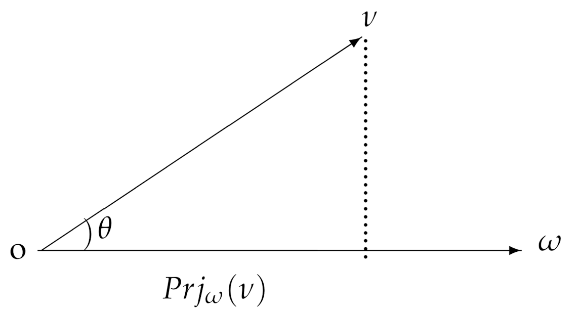
Step 5. Calculate the projection $Pro{j}_{A^{+}}\left(V^k\right)$ of $A^{+}$$(k\in T)$ on the PIS Vas follows:

$$Pr{j}_{A^{+}}\left(V^k\right)=\frac{{\sum }_{i=1}^m{\sum }_{j=1}^n{v}_{ij}^k{v}_{ij}^{+}}{\sqrt{{\sum }_{i=1}^m{\sum }_{j=1}^n{\left(v_{ij}^{+}\right)}^2}}$$

(19)

In a similar way, we compute the projection from the NIS.

Step 6. Next, compute the projection $Pro{j}_{A^{-}}\left(V^k\right)$ of $A^{-}$$(k\in T)$ on PIS V via:

$$Pr{j}_{A^{-}}\left(V^k\right)=\frac{{\sum }_{i=1}^m{\sum }_{j=1}^n{v}_{ij}^k{v}_{ij}^{-}}{\sqrt{{\sum }_{i=1}^m{\sum }_{j=1}^n{\left(v_{ij}^{-}\right)}^2}}$$

(20)

Step 7. Employ the values of $Pro{j}_{A^{+}}\left(V^k\right)$ and $Pro{j}_{A^{-}}\left(V^k\right)$ to determine a relative closeness to ranking all DMs. Similar to the TOPSIS method, each individual decision’s closeness in relation to $A^{+}$ is defined as:

$$R{C}_k=\frac{Pro{j}_{A^{-}}\left(V^k\right)}{Pro{j}_{A^{+}}\left(V^k\right)+Pro{j}_{A^{-}}\left(V^k\right)},k\in T$$

(21)

Step 8. It is clear that if $V_k$ is closer to $A^{+}$ and more remote from $A^{-}$, then $R{C}_k$ approaches one. Hence, by considering the relative closeness, we rank all members of the decision committee. Therefore, we define the weight of the kth DM as:

$${\lambda }_k=\frac{R{C}_k}{{\sum }_{k=1}^{t}R{C}_k},k\in T$$

(22)

Step 9. Finally, all decision matrices $V_k,k\in T,$ are integrated into a matrix V by:

$$V=\sum _{k=1}^t{\lambda }_k{V}_k={\left([{\underline{v}}_{ij},{\overline{v}}_{ij}]\right)}_{m\times n}$$

(23)

Next, we sum all interval numbers in each row of matrix V. Therefore, the total evaluation of alternative $A_i(i\in M)$ is derived:

$$v_i=[{\underline{v}}_i,{\overline{v}}_i]=\sum _{j=1}^n[{\underline{v}}_{ij},{\overline{v}}_{ij}],i\in M$$

(24)

Now, we employ Equation (3) to construct the matrix $P={\left[p_{ij}\right]}_{m\times m}$. Then, using Equation (4), all $v_i(i\in M)$ are ranked in descending order using the values of $p_i(i\in M)$. Finally, the alternatives are ranked by the $p_i$ values in descending order.

Comparing the Proposed Approach with Other Methods

Here, the proposed method in this study is compared with two different MCDM methods, the traditional TOPSIS and the extended TOPSIS proposed by Ye and Li [44], which are similar approaches to this research in the literature. These methods were selected as the background of the proposed method. Compared with the method of traditional TOPSIS and the approach proposed by Ye and Li, this method has several differences. First, the PIS and NIS in traditional TOPSIS are vectors, which are derived from alternatives, while in the proposed method, the PIS and NIS are matrices, which are derived from the decision matrices of all DMs. This description of the procedure of the proposed method is clear and simple for high-dimensional TOPSIS in the framework. Second, the relative importance of the DMs is different, and the weight of each DM is determined by his/her own decision matrix. When the decision matrix is closer to the PIS and farther away from the NIS, the decision is better; furthermore, the weight is greater. The best decision is made by a (some) pseudo-DM(s), whose decision is PIS (the average matrix of all group decision matrices). From this point of view, a DM’s decision matrix is closer to the PIS, that is to say, a decision matrix is closer to the average matrix of group decision matrices, then it is better to represent the majority in the mean sense; when a DM’s decision matrix is closer to the NIS, the decision has a larger bias in the mean sense; meanwhile, when the DM has maximum regret, the proposed method assigns low weights to those “false” or “biased” ones. Therefore, it is suitable for those situations in which the DM wants to have maximum group utility and minimum individual risk in the mean sense.

5. Application

In this section, we employ the proposed methodology to a real case related to air quality assessment in China. The Guangdong Environmental Monitoring Center, together with the Environmental Protection Department of the Hong Kong Special Administrative Region, established the Pearl River Delta Regional air quality monitoring network, which includes 16 automatic air quality monitoring stations.

All stations are equipped to evaluate the ambient concentrations of respirable suspended particulates (RSPs) such as PM${}_{10}$, sulfur dioxide (SO${}_2$), and nitrogen dioxide (NO${}_2$).

In what follows, a thorough assessment of the air quality is displayed within the said zone. We consider the monitoring stations (MSs) as the DMs, and for simplicity, we select three MSs from D = {$d_1,d_2,d_3$} = {Luhu Park, Wanqingsha, Tianhu}.

Table 1. Data collected from the Luhu Park monitoring station (MS).

	SO${}_2$	NO${}_2$	PM${}_{10}$
	LL     UL	LL     UL	LL     UL
$X_1$
$A_1$	[0.013, 0.129]	[0.028, 0.144]	[0.021, 0.136]
$A_2$	[0.013, 0.107]	[0.038, 0.139]	[0.047, 0.155]
$A_3$	[0.003, 0.042]	[0.018, 0.054]	[0.014, 0.150]
$X_2$
$A_1$	[0.040, 0.161]	[0.034, 0.093]	[0.047, 0.199]
$A_2$	[0.047, 0.127]	[0.040, 0.081]	[0.102, 0.206]
$A_3$	[0.0140, 0.113]	[0.016, 0.086]	[0.030, 0.187]
$X_3$
$A_1$	[0.006, 0.188]	[0.004, 0.053]	[0.003, 0.174]
$A_2$	[0.015, 0.046]	[0.001, 0.026]	[0.021, 0.157]
$A_3$	[0.009, 0.034]	[0.005, 0.019]	[0.011, 0.103]

shows the assessed values by [45,46,47]. The alternatives are the monthly air quality for the November 2017, 2018, and 2019. Hence, suppose A = {$A_1,A_2,A_3$} = {November of 2017, November of 2018, November of 2019} shows the alternatives and U = {$u_1,u_2,u_3$} = {$S{O}_2,N{O}_2,P{M}_{10}$} represents the attributes. The specific pollutants we chose for the analysis, as well as the data period are based on the data availability.

Evidently, all attributes are the cost type, and using Equations (8) and (9), Table 1 is normalized into

Table 2. Normalized data from the MSs.

	SO${}_2$	NO${}_2$	PM${}_{10}$
	LL     UL	LL     UL	LL     UL
$X_1$
$A_1$	[0.02326, 0.10714]	[0.12500, 0.85714]	[0.10294, 0.66667]
$A_2$	[0.02804, 0.07895]	[0.12950, 0.38298]	[0.09032, 0.29787]
$A_3$	[0.07140, 0.16667]	[0.33333, 1.28571]	[0.09333, 1.00000]
$X_2$
$A_1$	[0.08696, 0.35000]	[0.17204, 0.47059]	[0.15075, 0.63830]
$A_2$	[0.11024, 0.29787]	[0.19753, 0.40000]	[0.14563, 0.29412]
$A_3$	[0.12389, 1.00000]	[0.18605, 1.00000]	[0.16043, 1.00000]
$X_3$
$A_1$	[0.03191, 1.00000]	[0.01887, 0.25000]	[0.05660, 1.00000]
$A_2$	[0.13043, 0.40000]	[0.03846, 1.00000]	[0.11538, 0.14286]
$A_3$	[0.17647, 0.66667]	[0.05263, 0.20000]	[0.15789, 0.27273]

. We utilize Implementing Details for Urban Environmental Comprehensive Treatment and Quantitative Examination (GOSEPA, No. 36) to determine the weights of attributes. As a result, the weights of SO${}_2$, NO${}_2$, and PM${}_{10}$ are 0.4, 0.2, and 0.4, respectively.

Now, we use the weight vector $w=(w_1,w_2,w_3)=(0.4,0.2,0.4)$ to compute the weighted normalized decision matrix $R^k={\left([{\underline{r}}_{ij}^k,{\overline{r}}_{ij}^k]\right)}_{m\times n}(k=1,2,3)$. The results are shown in Table 2.

Next, the PIS and NIS, $A^{+}$ and $A^{-}$, are computed and respectively represented by

Table 3. Weighted normalized data obtained from the MSs.

	SO${}_2$	NO${}_2$	PM${}_{10}$
	LL     UL	LL     UL	LL     UL
$X_1$
$A_1$	[0.00930, 0.04286]	[0.02500, 0.17143]	[0.04118, 0.26667]
$A_2$	[0.01122, 0.03158]	[0.02590, 0.07660]	[0.03613, 0.11915]
$A_3$	[0.02856, 0.06667]	[0.06667, 0.25714]	[0.03733, 0.40000]
$X_2$
$A_1$	[0.03478, 0.14000]	[0.03441, 0.09412]	[0.06030, 0.25532]
$A_2$	[0.04410, 0.11915]	[0.03951, 0.08000]	[0.05825, 0.11765]
$A_3$	[0.04956, 0.40000]	[0.03721, 0.20000]	[0.06417, 0.40000]
$X_3$
$A_1$	[0.01276, 0.40000]	[0.00377, 0.05000]	[0.02264, 0.40000]
$A_2$	[0.05217, 0.16000]	[0.00769, 0.20000]	[0.04615, 0.05714]
$A_3$	[0.07059, 0.26667]	[0.01053, 0.04000]	[0.06316, 0.10909]

,

Table 4. Positive ideal solution (PIS) $A^{+}$.

	SO${}_2$	NO${}_2$	PM${}_{10}$
	LL     UL	LL     UL	LL     UL
$A_1$	[0.00930, 0.04286]	[0.00377, 0.05000]	[0.02264, 0.25532]
$A_2$	[0.01122, 0.03158]	[0.00769, 0.07660]	[0.03613, 0.05714]
$A_3$	[0.02856, 0.06667]	[0.01053, 0.04000]	[0.03733, 0.10909]

and

Table 5. Negative ideal solution (NIS) $A^{-}$.

	SO${}_2$	NO${}_2$	PM${}_{10}$
	LL     UL	LL     UL	LL     UL
$A_1$	[0.03478, 0.40000]	[0.03441, 0.17143]	[0.06030, 0.40000]
$A_2$	[0.05217, 0.16000]	[0.03951, 0.20000]	[0.05825, 0.11915]
$A_3$	[0.07059, 0.40000]	[0.06667, 0.25714]	[0.06417, 0.40000]

.

The next step is calculating the projection of each weighted normalized decision matrix on the PIS. Table 5 and

Table 6. Projections.

Projections	${\mathit{X}}_1$	${\mathit{X}}_2$	${\mathit{X}}_3$
$Pr{j}_{A^{+}}\left(V^k\right)$	0.17018	0.19581	0.20060
$Pr{j}_{A^{-}}\left(V^k\right)$	1.43006	1.93523	1.81254

present the results.

Now, we utilize Steps 7 and 8 to compute the relative closeness and weights of MSs, and the results are given in

Table 7. Relative closeness, weight, and ranking of the MSs.

MS	${\mathit{RC}}_{\mathit{k}}$	${\mathit{\lambda }}_{\mathit{k}}$	Ranking
$X_1$	0.89365	0.33072	3
$X_2$	0.90812	0.33608	1
$X_3$	0.90035	0.33320	2

. The weight vector $\lambda =({\lambda }_1,{\lambda }_2,{\lambda }_3)=(0.33072,0.33608,0.33320)$ and Equation (24) are employed to combine the individual decision matrices $V_1,V_2$, and $V_3$ into a decision matrix V (see

Table 8. Decision matrix V.

	SO${}_2$	NO${}_2$	PM${}_{10}$
	LL     UL	LL     UL	LL     UL
$A_1$	[0.01902, 0.19451]	[0.02109, 0.10499]	[0.04143, 0.30728]
$A_2$	[0.03591, 0.10380]	[0.02441, 0.11886]	[0.04690, 0.09798]
$A_3$	[0.04962, 0.24534]	[0.03806, 0.16559]	[0.05496, 0.30307]

).

The total interval evaluation of each alternative is obtained by summing all components in each row of Table 8, and consequently, we have ${\nu }_1=[0.08154,0.60678],{\nu }_2=[0.10722,0.32064],{\nu }_3=[0.14264,0.71400]$.

Using Equation (2), each ${\nu }_i$ is compared with the other ${\nu }_j(j=1,2,3)$ to drive the rank interval numbers ${\nu }_i(i=1,2,3)$. Therefore, by Equation (3), the matrix P is constructed:

$$P=\left(\begin{array}{ccc}0.50000& 0.67631& 0.42325\\ 0.32369& 0.50000& 0.22682\\ 0.57675& 0.77318& 0.50000\end{array}\right)$$

Now, Equation (4) is employed, and as a result, $p_1=1.59956$, $p_2=1.05051$, $p_3=1.84993$. Using the values of $p_i(i=1,2,3)$, the ${\nu }_i(i=1,2,3)$ are ranked in descending order; that is, ${\nu }_3>{\nu }_2>{\nu }_1$. Finally, the alternatives $A_i(i=1,2,3)$ are ranked as: $A_3>A_1>A_2.$ This means that $A_3$ is the best alternative. In other words, November 2019 had the best air quality. Our results are partly in line with Gao et al. [38]; however, our study provides a further extension in a very significant manner by using the most recent data, as well as a more advanced technique.

6. Conclusions

Because of the massive economic activities in different industrial sectors, the air pollution in China is still an important issue, being not only a concern of the government for sustainable development, but also a concern of the Chinese citizens for their health. The most recent research shows that because of the outbreak of the coronavirus at the beginning of 2020 together with the extremely strict rules implemented by the Chinese government in the process of the national lockdown, the pollutant concentrations in Shanghai reduced during the lockdown period; however, it was still four-times higher than the standard set out by the World Health Organization [48]. Therefore, the air pollution is still a very serious issue affecting people’s daily lives. How to reduce the level of pollution is the main question faced by the Chinese government and environmental regulatory authority. Before implementing relevant plans to address this issue, the correct information regarding the level of pollution should be provided, which requires a robust estimation or assessment of the air pollution level. The current study attempted to evaluate the level of air pollution by proposing an innovative multiple criteria decision making model, namely the group multiple criteria decision making model, in which the decision makers’ weights or preferences regarding different air pollution criteria can be quantified. We further applied our innovative model to a sample of data from the Pearl River Delta Region by focusing on three different pollutants, NO${}_2$, SO${}_2$, and PM${}_{10}$, for November 2017, 2018, and 2019. The results from our model show that November 2019 had the best air quality. We propose policy implications to the Chinese government in order to deal with this pollution issue: (1) although the Chinese government and regulatory authority have been closely monitoring and implementing relevant environmental laws to regulate air pollution, the magnitude should be further enhanced by increasing the amounts of fines on air pollution; at the current stage, the penalty is less than that in Europe (China Proposes Tiny $4500 Fine for Carbon Market Cheaters—Bloomberg); (2) the Chinese government should further enhance its research and development in clean energy; the use of clean energy will significantly reduce traditional energy production and further reduce the pollution level.

References

1. Katulski, R.J.; Namiesnik, J.; Sadowski, J.; Stefnski, J.; Wardencki, W. Monitoring of Gaseous Air Pollution. The Impact of Air Pollution on Health, Economy, Environment and Agricultural Sources; IntechOpen: London, UK, 2011; p. 143. [Google Scholar]
2. Choi, S.; Baek, S.; Chang, Y.; Wania, F. Passive air sampling of polychlorinated biphenyls and organochlorine pesticides at the Korean arctic and antarctic research stations: Implications for long-range transport and local pollution. Environ. Sci. Technol. 2008, 42, 7125–7131. [Google Scholar] [CrossRef]
3. Ortolani, C.; Vitale, M. The importance of local scale for assessing, monitoring and predicting of air quality in urban areas. Sustain. Cities Soc. 2016, 26, 150–160. [Google Scholar] [CrossRef]
4. Potapowicz, J.; Lambropoulou, D.; Nannou, C.; Koziol, K.; Polkowska, Z. Occurrences, sources, and transport of organochlorine pesticides in the aquatic environment of Antarctica. Sci. Total Environ. 2000, 735, 139475. [Google Scholar] [CrossRef] [PubMed]
5. Wang, Q.; Dai, H.N.; Wang, H. A smart MCDM framework to evaluate the impact of air pollution on city sustainability: A case study from China. Sustainability 2017, 9, 911. [Google Scholar] [CrossRef] [Green Version]
6. Chen, L.; Shi, M.; Gao, S.; Li, S.; Mao, J.; Zhang, H.; Sun, Y.; Bai, Z.; Wang, Z. Assessment of population exposure to PM2.5 for mortality in China and its public health benefit based on BenMAP. Environ. Pollut. 2017, 221, 311–317. [Google Scholar] [CrossRef]
7. India, Russia, China among Top Sulfur Dioxide Emitters. Available online: https://www.euronews.com/2019/08/23/india-russia-china-among-top-sulfur-dioxide-emitters-report (accessed on 23 August 2019).
8. Fan, H.; Zhao, C.; Yang, Y. A comprehensive analysis of the spatio-temporal variation of urban air pollution in China during 2014–2018. Atmos. Environ. 2020, 220, 117066. [Google Scholar] [CrossRef]
9. Guan, D.; Su, X.; Zhang, Q.; Peters, G.P.; Liu, Z.; Lei, Y.; He, K. The socioeconomic drivers of China’s primary PM2.5 emissions. Environ. Res. Let. 2014, 9, 024010. [Google Scholar] [CrossRef] [Green Version]
10. Liu, Y.; Zheng, M.; Yu, M.Y.; Cai, X.H.; Du, H.Y.; Li, J.; Zhou, T.; Yan, C.Q.; Wang, X.S.; Shi, Z.B.; et al. High-time-resolution source apportionment of PM2.5 in Beijing with multiple models. Atmos. Chem. Phys. 2019, 19, 6595–6609. [Google Scholar] [CrossRef] [Green Version]
11. Karplus, V.J.; Zhang, S.; Almond, D. Quantifying coal power plant responses to tighter SO2 emissions standards in China. Proc. Natl. Acad. Sci. USA 2018, 115, 7004–7009. [Google Scholar] [CrossRef] [Green Version]
12. Li, R.; Fu, H.B.; Cui, L.L.; Li, J.L.; Wu, Y.; Meng, Y.; Wang, Y.T.; Chen, J.M. The spatiotemporal variation and key factors of SO2 in 336 cities across China. J. Clean. Prod. 2019, 210, 602–611. [Google Scholar] [CrossRef]
13. Zheng, C.W.; Zhao, C.F.; Li, Y.P.; Wu, X.L.; Zhang, K.Y.; Gao, J.; Qiao, Q.; Ren, Y.Z.; Zhang, X.; Chai, F.H. Spatial and temporal distribution of NO2 and SO2 in Inner Mongolia urban agglomeration obtained from satellite remote sensing and ground observations. Atmos. Environ. 2018, 188, 50–59. [Google Scholar] [CrossRef] [Green Version]
14. Niroomand, S.; Hadi-Vencheh, A.; Şahin, R.; Vizvári, B. Modified migrating birds optimization algorithm for closed loop layout with exact distances in flexible manufacturing systems. Expert Syst. Appl. 2015, 42, 6586–6597. [Google Scholar] [CrossRef]
15. Wanke, P.; Alvarenga, H.; Correa, H.; Hadi-Vencheh, A.; Azad, M.A.K. Fuzzy inference systems and inventory allocation decisions: Exploring the impact of priority rules on total costs and service levels. Expert Syst. Appl. 2017, 85, 182–193. [Google Scholar] [CrossRef]
16. Wanke, P.; Chen, Z.; Zheng, X.; Antunes, J. Sustainability efficiency and carbon inequality of the Chinese transportation system: A Robust Bayesian Stochastic Frontier Analysis. J. Environ. Manag. 2020, 260, 110163. [Google Scholar] [CrossRef] [PubMed]
17. Yousefi, A.; Hadi-Vencheh, A. An integrated group decision making model and its evaluation by DEA for automobile industry. Expert Syst. Appl. 2010, 37, 8543–8556. [Google Scholar] [CrossRef]
18. Zareei, A.; Zaerpour, F.; Bagherpour, M.; Noora, A.A.; Hadi-Vencheh, A. A new approach for solving fuzzy critical path problem using analysis of events. Expert Syst. Appl. 2011, 38, 87–93. [Google Scholar] [CrossRef]
19. French, J.R.P. A formal theory of social power. Psychol. Rev. 1965, 63, 181–194. [Google Scholar] [CrossRef]
20. Theil, H. On the symmetry approach to the committee decision problem. Manag. Sci. 1963, 9, 380–393. [Google Scholar] [CrossRef]
21. Keeney, R.L.; Kirkwood, C.W. Group decision making using cardinal social welfare functions. Manag. Sci. 1975, 22, 430–437. [Google Scholar] [CrossRef]
22. Ramanathan, R.; Ganesh, L.S. Group preference aggregation methods employed in AHP: An evaluation and an intrinsic process for deriving members’ weightages. Eur. J. Oper. Res. 1994, 79, 249–265. [Google Scholar] [CrossRef]
23. Martel, J.M.; Ben Khelifa, S. Deux Propositions D’aide multicritère à la Dècision de Groupe; Ben Abdelaziz, B., Et Mellouli, H., Eds.; Optimisation et Decision, Centre de Publication Universitaire: Tunis, Tunisia, 2000; pp. 213–228. [Google Scholar]
24. Xu, Z.S. Group decision making based on multiple types of linguistic preference relations. Inform. Sci. 2008, 178, 452–467. [Google Scholar] [CrossRef]
25. Chen, X.; Fan, Z.P. Study on assessment level of experts based on difference preference information. Syst. Eng. Theory Pract. 2007, 27, 27–35. [Google Scholar] [CrossRef]
26. Xu, Z. On method for uncertain multiple attribute decision making problems with uncertain multiplicative preference information on alternatives. Fuzzy Optim. Decis. Mak. 2005, 4, 131–139. [Google Scholar] [CrossRef]
27. Saffarzadeh, S.; Hadi-Vencheh, A.; Jamshidi, A. An Interval Based Score Method for Multiple Criteria Decision Making Problems. Int. J. Inform. Technol. Decis. Mak. 2019, 18, 1667–1687. [Google Scholar] [CrossRef]
28. Chen, L.; Pan, W. BIM-aided variable fuzzy multi-criteria decision making of low-carbon building measures selection. Sustain. Cities Soc. 2016, 27, 222–232. [Google Scholar] [CrossRef]
29. Allen, R.W.; Gombojav, E.; BarkhasragChaa, B.; Byambaa, T.; Lkhasuren, O.; Amram, O.; Takaro, T.K.; Janes, C.R. An assessment of air pollution and its attributable mortality in Ulaanbaatar, Mongolia. Air Qual. Atmos. Health 2013, 6, 137–150. [Google Scholar] [CrossRef] [PubMed] [Green Version]
30. Johnson, M.; Isakov, V.; Touma, J.S.; Mukerjee, S.; Ozkaynak, H. Evaluation of land-use regression models used to predict air quality concentrations in an urban area. Atmos. Environ. 2010, 44, 3660–3668. [Google Scholar] [CrossRef]
31. Son, Y.; Osornio-Vargas, A.; O’Neill, M.S.; Hystad, P.; Texcalac-Sangrador, J.L.; Ohman-Strickland, P.; Meng, Q.; Schwander, S. Land use regression models to assess air pollution exposure in Mexico City using finer spatial and temporal input parameters. Sci. Total Environ. 2018, 639, 40–48. [Google Scholar] [CrossRef] [PubMed]
32. Battista, G.; Pagliaroli, T.; Mauri, L.; Basilicata, C.; Vollaro, R.D.L. Assessment of the air pollution level in the city of Rome (Italy). Sustainability 2016, 8, 838. [Google Scholar] [CrossRef] [Green Version]
33. Dominick, D.; Juahir, H.; Latif, M.T.; Zain, S.M.; Aris, A.Z. Spatial assessment of air quality patterns in Malaysia using multivariate analysis. Atmos. Environ. 2012, 60, 172–181. [Google Scholar] [CrossRef]
34. Rahman, S.R.A.; Ismail, S.N.S.; Raml, M.F.; Latif, M.T.; Abidin, E.Z.; Praveena, S.M. The assessment of Ambient air pollution trend in Klang Valley, Amlaysia. World Environ. 2015, 5, 1–11. [Google Scholar]
35. Lawrence, A.; Fatima, N. Urban air pollution and its assessment in Lucknow city- The second largest city of North India. Sci. Total Environ. 2014, 488–489, 447–455. [Google Scholar] [CrossRef] [PubMed]
36. Vedrenne, M.; Borge, R.; Lumbreras, J.; Rodriguez, M.E. Advancements in the design and validation of an air pollution integrated assessment model for Spain. Environ. Model. Soft. 2014, 57, 177–191. [Google Scholar] [CrossRef] [Green Version]
37. Wang, L.; Zhang, P.; Tan, S.; Zhao, X.; Cheng, D.; Wei, W.; Su, J.; Pan, X. Assessment of urban air quality in China using air pollution indices (APIs). J. Air Waste Manag. Assoc. 2013, 63, 170–178. [Google Scholar] [CrossRef] [PubMed] [Green Version]
38. Gao, H.; Yang, W.; Yang, Y.; Yuan, G. Analysis of the air quality and the effect of governance policies in China’s Pearl River Delta, 2015–2018. Atmosphere 2019, 10, 412. [Google Scholar] [CrossRef] [Green Version]
39. Fang, D.; Wang, Q.; Li, H.; Yu, Y.; Lu, Y.; Qian, X. Mortality effects assessment of ambient PM2.5 pollution in the 74 leading cities of China. Sci. Total Environ. 2016, 569–570, 1545–1552. [Google Scholar] [CrossRef]
40. Gu, Y.; Yim, S.H.L. The air quality and health impacts of domestic trans-boundary pollution in various regions of China. Environ. Int. 2016, 97, 117–124. [Google Scholar] [CrossRef]
41. Chen, R.; Kan, H.; Chen, B.; Huang, W.; Bai, Z.; Song, G.; Pan, G. Association of particulate air pollution with daily mortality: The China air pollution and health effects study. Am. J. Epidemiol. 2012, 175, 1173–1181. [Google Scholar] [CrossRef] [PubMed]
42. Sueyoshi, T.; Yuan, Y. China’s regional sustainability and diversified resource allocation: DEA environmental assessment on economic development and air pollution. Energy Econ. 2015, 49, 239–256. [Google Scholar] [CrossRef]
43. Abootalebi, S.; Hadi-Vencheh, A.; Jamshidi, A. Ranking the alternatives with a modified TOPSIS method in multiple attribute decision making problems. IEEE Trans. Eng. Manag. 2019. [Google Scholar] [CrossRef]
44. Ye, F.; Li, Y.N. Group multi-attribute decision model to partner selection in the formation of virtual enterprise under incomplete information. Expert Syst. Appl. 2009, 36, 9350–9357. [Google Scholar]
45. GDEMC; HKEPD. A Report of Monitoring Results in 2017, Pearl River Delta Regional Air Quality Monitoring Network. 2017. Available online: www.gdepb.gov.cn/gsgg/201710/t20171026_49978.html (accessed on 13 March 2018).
46. GDEMC; HKEPD. A Report of Monitoring Results in 2018, Pearl River Delta Regional Air Quality Monitoring Network. 2018. Available online: www.gdepb.gov.cn/gsgg/201810/t20181026_49978.html (accessed on 17 August 2019).
47. GDEMC; HKEPD. A Report of Monitoring Results in 2019, Pearl River Delta Regional Air Quality Monitoring Network. 2019. Available online: www.gdepb.gov.cn/gsgg/201910/t20191026_49978.html (accessed on 17 September 2020).
48. Filonchyk, M.; Peterson, M. Air Quality Changes in Shanghai, China, and the Surrounding Urban Agglomeration During the COVID-19 Lockdown. J. Geovis. Spat. Anal. 2020, 4, 22. [Google Scholar] [CrossRef]
Figure 1. Projection of vector ν and ω .
Sustainability 13 01686 g001