1. Introduction
Our world has experienced remarkable economic growth since the industrial revolution, achieving the world’s all-time highest global living standards and income per capita. However, economic prosperity came with an excessive cost, where the fossil-based capitalism triggered greenhouse gas emissions and resulted in climate change that is familiar nowadays. Nevertheless, countries, especially developing countries that are not the main contributors to the current climate change crisis, hesitate to deter their own economic growth. Instead, countries seek a new growth strategy where economic growth can be proceeded along with environmental conservation. This strategy is well known with various names such as green growth [
1,
2,
3,
4], green economy [
5] and inclusive green growth [
6]. This is in contrast with the degrowth movement that criticizes the economic growth strategy at all costs [
7].
The major issue of the green growth strategy is the different perspective on economic growth between the developed and developing countries. Developed countries with high income per capita tend to pursue an eco-friendly economic growth strategy along with environmental policies such as environmental tax and removal of fossil fuel subsidies. They intend to impose tariffs on imports of non-eco-friendly goods, which are known as the border tax. However, developing countries that maintain the traditional growth strategy cannot follow this green growth strategy due to insufficient green technology and financial resources. Since their economic growth depends much on global trade, especially on exports to the developed countries, it is important to derive international cooperation in green technology and investment with developed countries by proactively persuading developing countries to pursue the green growth strategy [
8].
Classifying industries into green and non-green industries, this paper investigates the trend of exports of green goods and the determinants of its exports. The trade data were collected bilaterally. The classification of green goods was from the GGS (Green Goods and Services) of the U.S. BLS [
9], and then they were matched with the NAICS (North American Industry Classification System) 2012 and the SITC (Standard International Trade Classification) Rev.2 codes [
8]. With the bilateral trade data of the green goods, the gravity model specification with the PPML (Poisson pseudo-maximum likelihood) was estimated to examine the impacts of two environmental policy indicators which are defined as the ratio of environmental tax revenue to GDP and energy intensity as a ratio of supply of primary energy to GDP.
There are many studies on the impact of environmental policies on trade [
10,
11,
12,
13,
14,
15,
16]. Their findings are quite diverse, depending on the coverage of countries, definition of environmental policy indicators and coverage of trade sectors, etc. For example, Van Beers and Van den Bergh [
10] found a negative effect of energy intensity as an environmental indicator on trade but no robust effect on trade in dirty industries.
In terms of the coverage of countries, definition of green industries and estimation methodology, this study differed from other related papers in the effects of environmental policies on general trade.
To be specific, existing studies generally examined the determinants of general trade and utilized simple OLS (Ordinary Least Squares) estimation with fixed effect using dummy variables. The major concern of OLS estimation is the heteroskedasticity issue caused by zero trade data. On the other hand, the significance of this study lies in not only classifying industries into green and non-green industries but also utilizing the PPML estimation method, which is a more appropriate empirical analysis method than the OLS.
Furthermore, existing studies tend to analyze the impact of environmental policies in all countries without considering the country’s characteristics. However, countries that share similar characteristics like income level are likely to implement similar environmental policies, and therefore, when analyzing the impact of policies, it is critical to apply different policy standards for each country. Therefore, this study utilized bilateral data and focused on investigating bilateral green exports among the developed and developing countries. In detail, dependent variables were assumed as general bilateral green exports, bilateral green exports of developed to developed or developing countries and bilateral exports among developing countries.
The empirical findings on two different environmental policy indicators depended on green trade patterns. First of all, two environmental indicators were assumed: the share of environmentally related tax revenue to GDP and the energy intensity ratio which is defined as the energy demand to GDP. Environmental interpretation of the two indicators is opposite. Higher environmental tax indicates that the government enforces stronger environmental policies while higher energy intensity indicates that the economy is less efficient from the environmental perspective. The environmental tax indicators showed statistically significant and positive coefficients for exporting countries between HIC (high-income countries) for all green trade patterns. However, energy intensity for world green exports among all countries showed a positive and significant coefficient for importing countries but not significant for exporting countries. The coefficient for energy intensity for bilateral green exports showed diverse results. For exports among HIC, the coefficient for energy intensity showed a positive and statistically significant coefficient for importing but no significant coefficient for exporting countries. For bilateral green exports from HIC to LMY (low- and middle-income) countries, energy intensity showed a negative and statistically significant coefficient for both exporting and importing countries. For bilateral green exports between LMY countries, energy intensity was shown to be positive and significant for both exporting and importing countries. However, for bilateral green exports from LMY countries to HIC, energy intensity was not shown to be significant.
This paper is organized as follows.
Section 2 summarizes the literature on green growth strategy and related empirical estimation results.
Section 3 describes the classification of green industries and their descriptive statistics.
Section 4 explains data and empirical model specification,
Section 5 discusses the estimation results, and
Section 6 concludes.
2. Green Growth and Trade
As we see from the Paris Agreement, which is referred to as the post-2020 New Climate Regime and the Net Zero 2050, the international community realizes how serious climate change and its impacts on the economy and health are. For example, Zhang et al. [
17] found that the number of premature deaths related to particulate matter with a diameter of 2.5 micrometers or less PM
2.5 was 3.45 million in 2007; 762,400 (about 22%) of them originated from consumption of goods and services that are produced and imported from another region. There are many related studies on the impacts of environmental factors on health [
18,
19].
Even under the harmful effects on health, most countries, in particular developing countries, are quite eager to continue the economic growth strategy. Therefore, the issue is how we can achieve sustainable economic growth within the changing growth paradigms. On the one hand, as one of the alternative development models and often referred to as the traditional strategy, degrowth strategy argues that environmental conservation cannot proceed along with economic growth, however, society can still sustain economic stability without economic growth [
20]. The term “degrowth” in the concept of climate change arose from criticizing the global capitalist system that caused various environmental challenges.
On the other hand, by demonstrating the Great Recession and Japan’s zero growth as examples, Pollin [
7] pointed out that global GDP contraction can simply lead to huge job losses and a decline in the standard of living without any environmental improvement. Rather, he argued that converting the fossil-fuel-dominant infrastructure and fossil-fuel consumption to viable alternatives can be accomplished through the Green New Deal project along with economic growth. Specifically, the Green New Deal project seeks for the global initiative to invest a proportion of global GDP (1.5~2%) in the clean energy transition to eliminate or absolutely decouple CO
2 emissions and improve living standards by lowering the energy consumption price. This program asserts that faster economic growth will increase the amount of investment, thus accelerating the clean energy transition. Further, the clean energy transition will lay off workers in the current fossil-fuel-based energy sector but, at the same time, bring new job opportunities in various forms. Pollin [
21] pointed out that strong clean energy industrial policies are required for this project to succeed and economic growth can proceed along with clean energy transition under the Green New Deal project.
Like the Green New Deal, the new growth strategy should be an eco-friendly growth paradigm that motivates the synergic relationship between economic growth and the environment. This type of strategy is called green growth, green economy or inclusive green growth strategy. The green growth term was first introduced in the title of Ekins’ book [
1] and was recommended as a growth strategy by UN ESCAP in 2005 [
22]. It was selected as a comprehensive economic development strategy in the Republic of Korea in 2009, which is called the “Low Carbon, Green Growth” strategy [
2,
22]. UNEP (United Nations Environment Programme) [
5] presents a different term “Green Economy” which is quite similar to the green growth formally mentioned. The World Bank [
6] suggests inclusive green growth which is similar to both green growth and green economy concepts but considers social value in addition.
As the circular economy concept received great interest quite recently, Kirchherr et al. [
23] analyzed 114 circular economy definitions suggested by different studies and conceptualized the circular economy. They proposed a unified circular economy definition, which is a concept based on a business model that replaced linear economy and operates at the micro level, meso level and macro level to achieve sustainable development. Figge et al. [
24] pointed out that the eco-efficiency in linear systems examined by existing studies is underestimated in circular systems and is not properly measured. They suggested that micro-level contributions to resource flows and interaction between firms that improve the overall degree of eco-efficiency within the circular economy should be considered to calculate eco-efficiency in the circular approach.
All countries, developing or developed, that agree to adopt green growth strategies face difficulty in switching to green growth strategies. However, developing countries with traditional growth strategies due to insufficient financial resources and technologies face difficulties in switching to green growth strategies. In this case, it is necessary to provide various international support from developed countries and persuade the developing countries to seek eco-friendly production strategies. This strategy can be justified in two ways. First, developed countries have tried to introduce environmental tax for domestically produced goods as well as imported goods. Second, since developing countries can sustain economic growth through global trade with developed countries, it is necessary for them to produce export goods in eco-friendly ways.
There are few studies that investigate the impacts of environmental regulations on trade and the impacts on green trade utilizing bilateral trade data among the developed and developing countries. The related studies are reviewed as follows.
By estimating the gravity model for the OECD (Organisation for Economic Co-operation and Development) countries with country fixed effects and year fixed effects, Van Beers and Van den Bergh [
10] found that environmental regulation measured by energy intensity shows negative effects on the trade of aggregate and footloose industries but shows an insignificant effect on the trade of dirty industries. Extending the model above, Harris et al. [
11] analyzed the impacts of environmental regulations on bilateral trade among the OECD countries for 1990–1996. The environmental indicator which is defined as relative energy consumption and supply with consideration of country fixed effects does not show significant relation with trade. Grether and De Melo [
25] supported this argument by showing the non-robustness relationship between the regulatory gap and trade flows when additional control variables and their potential endogeneity are considered.
Jug and Mirza [
12] showed that for 12 EU and other 19 exporting countries in the period 1996–1999, more stringent environmental regulations measured by current environment expenditure tend to reduce exports and the coefficient is larger for the exporting countries such as Central and Eastern European countries. In addition, they showed that there is no significant difference in the impact of regulations on the trade of clean and dirty sectors. Tsurumi et al. [
14] found that energy intensity tends to reduce trade and GDP. Cantore and Cheng [
15] found that the environmental regulatory stringency plays an important role in the trade of environmental goods. The collected data for 71 countries and environmental goods were classified by the OECD for 1999–2014.
Costantini and Crespi [
26] employed the gravity model to investigate the impact of environmental regulation on the export of the energy sector of 20 OECD countries from 1996 to 2005. They utilized OECD classification HS1996 to restrict the sample to energy-related technologies and included other explanatory variables such as GDP, population size, distance, past colonial experience, total country area, the number of energy-related patents (as a proxy for innovation) and CO2 emissions level (as a proxy for regulation efficiency measure). Empirical results show a positive and significant impact of stringent environmental regulations on environment-friendly export. In the same line, Costantini and Mazzanti [
27] explored the effect of various environmental regulations on the export of the major manufacturing sectors of 14 EU countries from 1996 to 2007. By also utilizing the gravity model, they found that specific energy taxes, environmental taxes and innovation incentives positively influence the export of the manufacturing sector, while the impact of overall environmental policies is not significant. Further strengthening the argument, Costantini et al. [
28] depicted regulations that are more comprehensive: demand-pull and technology-push are more effective, and thus should be pursued to promote export competitiveness.
The studies reviewed above investigated the effects of environmental policy indicators on general trade or dirty industries. However, they did not extend their analysis to the detailed classification of green and non-green industries. Extensive empirical analysis is conducted on the developed countries, especially on OECD and EU countries, as abundant data are available. Therefore, this study expanded the spatial scope by considering both developed and developing countries based on WB (World Bank) country classification by income level and comparing the result between the two groups.
3. Classification of Green and Non-Green Industries
Suffering from global resource waste and environmental destruction, green strategies such as green growth, green economy and inclusive green growth have increased rapidly. In addition, the circular economy approach suggests 3-R processes (reduce, reuse and recycle) as an alternative to the linear economy which is operated by take, make and dispose processes [
29]. In other words, the economy and environment should be balanced under a circular system, according to Boulding [
30]. Expanding this concept, changes in the production and use of products in accordance with the principle of the circular economy approach is the way to reduce environmental pollution. This study also emphasizes aspects of eco-friendly production and sustainability by analyzing the impact of environmental policies on green industry trade, and it can be said that the increase in exports contributes to economic growth. Therefore, as a precautionary procedure for analysis, we classified the industries as green and non-green in the following steps.
The green industry was classified by matching codes of the U.S. BLS classification and SITC [
8,
9,
31]. The green industry codes of NAICS 2012 were obtained from the classification of the U.S. BLS within five categories. They were (i) energy from renewable resources, (ii) energy efficiency, (iii) pollution reduction and removal, greenhouse gas reduction and recycling and reuse, (iv) natural resources and (v) environmental compliance, education and training and public awareness. Then these NAICS 2012 codes were matched with the SITC Rev.2 codes. The estimation was to analyze the impact of environmental regulation on bilateral green trade flows. The GGS indicates that green jobs are jobs in businesses that produce goods and provide services that benefit the environment or conserve natural resources which are defined by the U.S. BLS. This is identified from the survey to measure employment associated with the production of GGS from sampled business establishments. As a result, they confirm 325 industries (six-digit NAICS) as potential producers of GGS. The U.S. BLS provides more detailed information about GGS [
32]. This study selected category (iii) as a green industry, and it was matched with the SITC Rev.2 trade flows. This study aimed to analyze the effects of environmental policy on green trade. The purpose of environmental policy is to reduce natural pollution. For this, countries put effort to withhold tax or save energy during production. Category (iii) of the BLS sub-category is suitable for the classification of this study. In addition, there are 106 industries of category (iii) that account for a large portion of the total green classification (325 industries) by NAICS 2012 in Kang [
8]. Therefore, the number of green industries in this study is smaller than the number of original GGS defined by the U.S. BLS (325 industries).
Table 1 summarizes the share of the green industry codes based on the one-digit SITC Rev.2 classification. Out of the total 788 industries, the number of green industries is 106 with a share of 13.45%. The highest shares of green industries are SITC 6 (25.0%) and 7 (21.5%) with 45 and 26 industries, respectively. However, there are no green industries in four sectors: SITC 0, 1, 3 and 4.
The number of countries covered in this analysis varies by year from 105 countries in 1990 to 129 countries in 2019 with the largest number of countries in 2017, covering 179 countries.
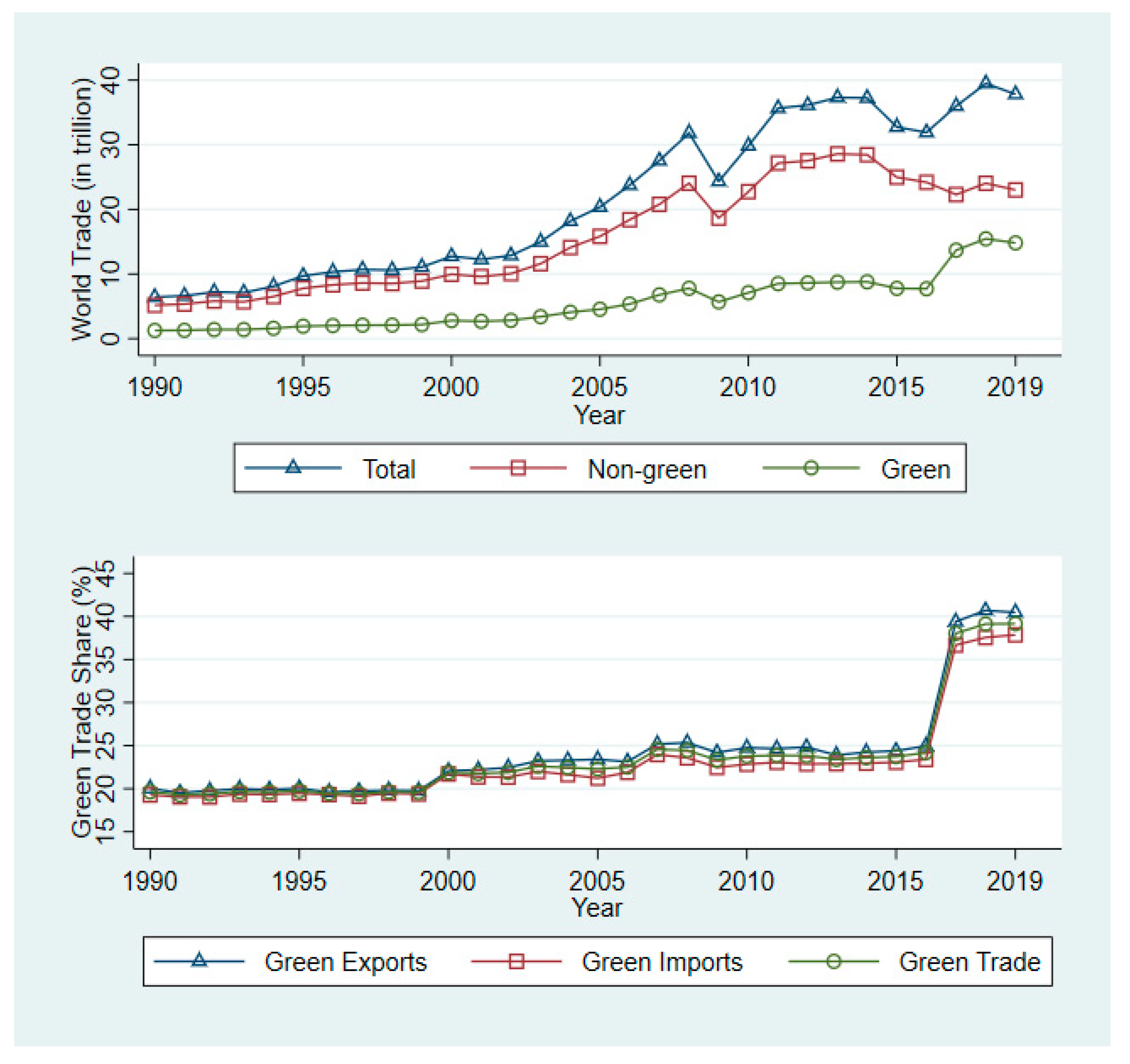
Figure 1 presents the increasing trends of green trade by whole, green and non-green classification for the years 1990 to 2019. The total amount of trade was USD 6.42 trillion in 1990, and the amounts of total green and non-green were USD 1.26 and USD 5.16 trillion, respectively. Green trade increased more than 11 times in 2019 since 1990, where it showed the largest increase among the three classifications reaching USD 14.81 trillion. The shares of green trade also showed an increasing trend since 1999 with a rapid increase in 2017.
Not only the share of green trade but every trend in the lower graph of
Figure 1 show a notable rise in 2017 and a similar trend throughout the period. The shares of green export, import and trade are calculated by dividing green trade volume (exports, imports and trade) by the total trade volume (exports, imports and trade), respectively. Thus, an increase in these shares implies the expansion of the global green industry from 1990 to 2019, with export contributing the most. In detail, the shares remained in an about 19% range in the 1990s but rose slightly since 2000. Then, the trends showed a small increase with some fluctuations from 2000 to 2016. In 2017, the shares of green exports, imports and trade rapidly increased, reaching 39.45%, 36.7% and 38.0%, respectively.
The radical change of data since 2017 is likely to be attributed to the amendment of the trade code. To be specific, collected data are classified according to the current classification and revision, then converted downward to the earlier classification code (see UN Comtrade homepage for a more detailed explanation on the code revision of UN Comtrade [
33]). The present classified trade code was reformed in 2017, reflecting the environmental and social issues of global concern. In other words, the trade code was enlarged to include a wider range of trade commodity types that are related to the environment. In addition, as this study classified the green industry based on SITC Revision 2, the data are not matched one to one, and thus the existence of potential bias should be considered.
The following graphs present the trend of bilateral trade between the HIC and the LMY countries. The classification of the countries is based on the principle of the World Bank Atlas method. This study categorized countries into two groups. By using the World Bank Atlas method, countries with USD 1035 or less in 2019 are classified as low-income countries; lower-middle-income economies are those with a GNI per capita between USD 1036 and USD 4045; upper-middle-income economies are those with a GNI per capita between USD 4046 and USD 12,535; high-income economies are those with a GNI per capita of USD 12,536 or more. The World Bank abbreviated the low-, lower-middle- and upper-middle-income countries as LMY and high-income countries as HIC [
34]. The HIC account for about 73% of global trade, and all types of trade trends have been decreasing since 1991 (about 83%), otherwise corresponding to LMY.
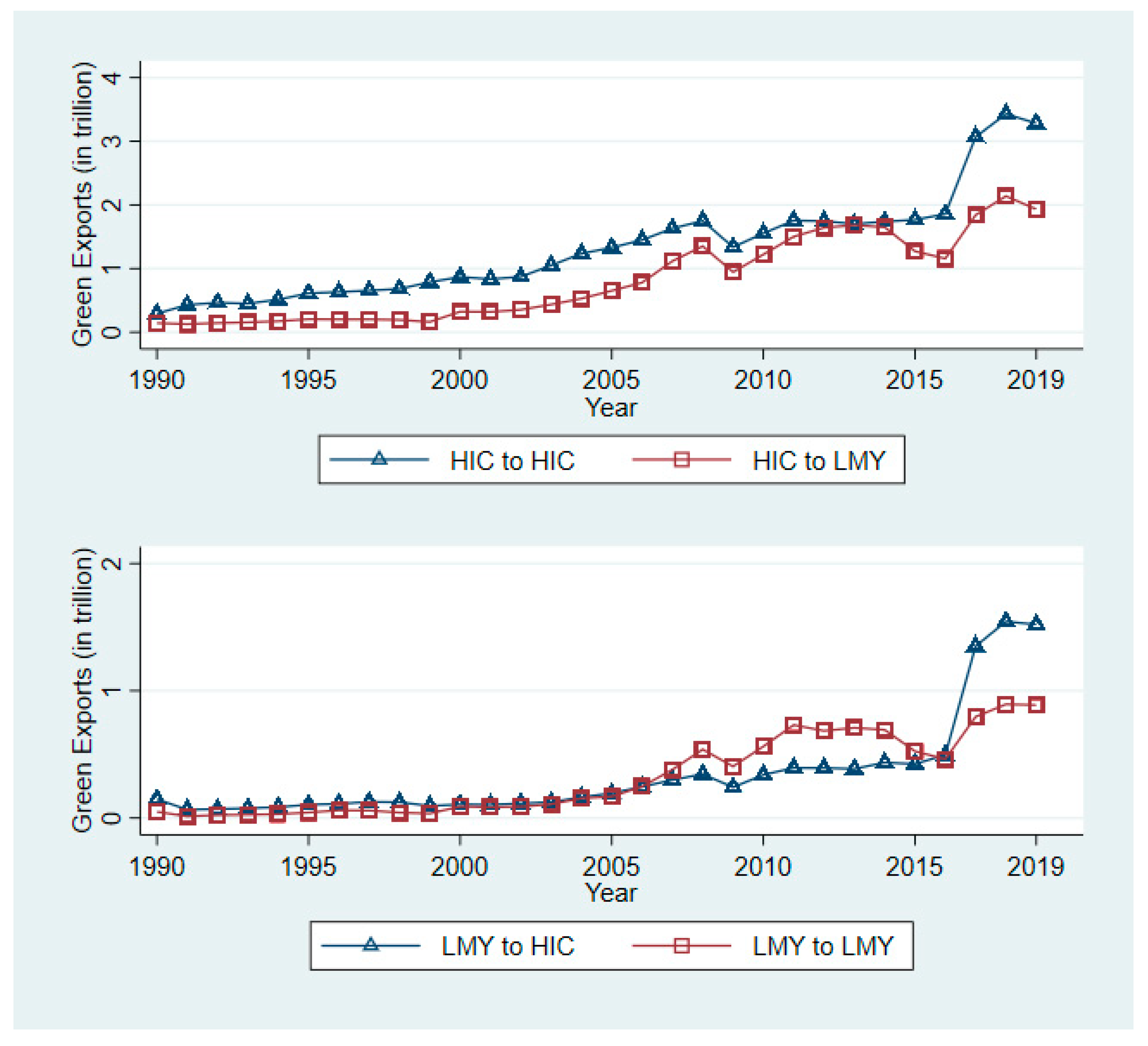
Figure 2 shows the bilateral green exports and imports (in trillion USD) between the classified countries. For green exports, every bilateral green export shows increasing trends from 1990 to 2019. The upper graph of
Figure 2 shows the bilateral green exports (in trillion USD) between HIC to HIC and HIC to LMY. In detail, the HIC-to-HIC trend increased from USD 0.29 trillion in 1990 to USD 3.28 trillion in 2019, showing a similar trend to the total world trade trend in
Figure 1. Green export from HIC to LMY increased from USD 0.14 trillion in 1990 to USD 1.93 trillion in 2019, demonstrating that the volume of green export between the HIC was much larger than the export from HIC to LMY throughout the period. Nevertheless, the gap between the two trends seems to decrease to as low as USD 0.02 trillion in 2013, although the gap started to increase again in 2016.
The lower graph of
Figure 2 shows the bilateral green export (in trillion) from the prospect of LMY countries. Similar to the upper graph that showed trends of green exports from the HIC viewpoint, trends of green exports from the LMY’s viewpoint also show an increasing trend throughout the period. In addition, the green export volume between the LMY countries was smaller than the green export volume from LMY to HIC, and the gap has rapidly increased since 2016. To be specific, green export between the LMY countries increased about 18 times from USD 0.05 trillion in 1990 to USD 0.89 trillion in 2019 and showed a gradual increase since 2016. On the other hand, green export volume from LMY to HIC increased about 10 times from 1990 to 2019, reaching USD 0.15 trillion and USD 1.52 trillion, respectively.
An important part of the international flows is intermediate products in the framework of global value chains (GVCs). Moreover, export added value varies by country because of the specializing and distributing production process of final goods to various countries. For this reason, countries with advanced eco-friendly technology can proactively promote export-driven strategy, participate in GVCs and reduce environmental pollution at the same time. Meanwhile, countries that are not equipped with high technology can only import to satisfy domestic demand. In other words, green industry and technology could affect the internationalization of production, and thus environmental policies could affect bilateral trade. Therefore, countries not equipped with eco-friendly technology should gradually participate in the GVCs by improving the environment of the industrial and production processes. Trade flow includes both final and intermediate goods, so it can be said that this study considers the GVCs as well.
4. Empirical Model Specification
The empirical model is adopted from the traditional gravity model with consideration of the exporter and importer fixed effects and year fixed effects [
35,
36]. According to the gravity literature, trade cost not only includes the trade distance between the two countries but also includes common language, colony, sharing a common land border, RTA (Regional Trade Agreements) and others. The baseline gravity model equation with exporter and importer fixed effects is based on Anderson and van Wincoop [
36] by controlling time-invariant variables which are called the MRFs because of possible bias. The model specification is as follows:
where
is the exporting country,
is the importing country, and
is the constant term.
refers to the trade volume from country
to country
, respectively.
and
indicate the GDPs of the exporter and the partner countries, respectively.
is trade cost between country
and country
. Various proxy indicators for trade cost are used in the literature with the gravity model, which are common language, colony, a common land border, RTA, etc.
indicates a vector of the factors that affect trade, including economic size and environmental factors.
and
stand for the multilateral resistance terms which include exporter and importer fixed effects.
,
and
are the coefficients to be estimated.
Taking natural log for Equation (1), the following empirical model specification with the stochastic term in year
is derived:
where
is a constant term. The stochastic error term includes time-fixed term (
) and white noise (
) as follows.
The dependent variable is the logarithm of green export flows from country to country in year because this study aimed to find the determinants of green exports.
Control variables in Equation (2) are summarized as follows.
First,
and
in year
are the proxy of the economic size of the two countries. The data are obtained from the World Bank WDI (World Development Indicators) [
37]. For exporting counties, it means a potential supply and potential demand for partner countries. The GDP coefficients are expected to be positive.
Second, ( is the logarithm of the population weighted bilateral distance between trade countries i and j in year t representing trade resistance, which is expected to be negative.
Third, there are four MRF variables: (i)
is a dummy variable for using common official or primary language between countries
i and
j; (ii)
is a dummy variable that countries
i and
j have ever been in a colonial relationship; (iii)
is a dummy variable indicating the presence of a contingent, i.e., sharing a common land border; and (iv)
is a dummy variable, equal to 1 if countries
i and
j are members of FTA/WTO in time
t. These are expected to be positive because of sharing factors of trading countries. The distance and MRF variables are available from CEPII (Centre d’ Études Prospectives et d’Informations Internationales) [
38].
Fourth, two proxy indicators as environmental regulation (environmental tax and energy intensity) are assumed. The effects of environmental regulation on trade vary by studies. The first one is environmentally related taxes which is defined as a percentage of environmentally related tax revenue to GDP (
,
collected from OECD statistics [
39]. Several estimated values were treated as missing because of over-identification. Environmentally related taxes include: (i) energy products (including vehicle fuels); (ii) motor vehicles and transport services; (iii) measured or estimated emissions to air and water, ozone-depleting substances, certain non-point sources of water pollution, waste management and noise, as well as management of water, land, soil, forests, biodiversity, wildlife and fish stocks.The data is available from the OECD Policy Instrument Database [
40].
The second one is energy intensity which is defined as the ratio of primary energy supply to GDP (
,
). It is defined as the ratio of energy primary supply (MJ) to GDP at 2017 PPP USD collected from WDI and OECD statistics [
37,
39]. Energy intensity indicates how much energy is used to produce one unit of economic output. A higher value of environmental indicators represents more stringent regulation, which is expected to result in a reduction in export or market competitiveness.
Finally, and are fixed effects in countries i and j in year t, is time effect, and is an error term with white noise disturbance.
Table 2 presents summary statistics of variables included in baseline model specification for 119 countries from 1990 to 2018.
5. Empirical Results
Most of the gravity models on the impacts of environmental policies on trade follow OLS estimation with consideration of country- and year-dummy effects. However, bilateral trade data classified by high-level digit codes include many zero trade volumes. In this case, the coefficients estimated by OLS estimation can have bias due to heteroscedasticity from zero trade values.
Silva and Tenreyro [
41,
42] recommended using the PPML approach to overcome the bias of the parameters estimated by OLS in the presence of heteroskedasticity leading to biased estimates of the true elasticities in the gravity model. In general, the Poisson regression method is used to count data of the dependent variable. However, it became more popular for the estimation of multiplicative models with different data as well [
42].
It should be noted that the PPML is different from the traditional Poisson estimation because the PPML drops the regressors if their (pseudo) maximum likelihood estimate does not exist. The estimation is conducted as follows [
42]. First, estimate the OLS regression for the observation with positive values of the dependent variable. Second, construct a subset of explanatory variables only with coefficients which can be estimated by step 1. Third, run the Poisson regression with this subset of regressors for the full sample. To check the adequacy of the estimated model specification, Silva and Tenreyro [
41] performed a heteroskedasticity-robust RESET (Regression Equation Specification Error Test).
The OLS and PPML estimation results are summarized in
Table 3 and
Table 4. To test the effects of data shifting between 1990–2016 and 2017–2019, we estimate the same model specifications in
Table 3 and
Table 4, but there is not much difference in the estimation results. Therefore, the results are not reported here but are available on request. For two tables, Model 1 shows OLS estimation results with exporting and importing country dummies and year dummies. The other five models are the PPML estimation results with fixed results. The estimated coefficients for all explanatory variables except for environmental indicators are shown to be consistent with those estimated by the same gravity model in other literature, and they have expected signs as well.
Table 3 shows the estimation result that used environmentally related taxes as the key explanatory variable. The estimation results in
Table 3 are summarized as follows.
The RESET test shows that the PPML models accept the null hypothesis at a 1% and 10% significant level, respectively (see Models 2 to 6). The null hypothesis is that the model does not suffer from misspecification [
41,
43]. As a result, the proxy measurement of the environmental regulation (
,
) appears significantly positive in exporting countries with a small coefficient of 0.578 between the HIC. In other words, it means that green exports increase when countries with environmentally sensitive regulation increase. This implies that promoting green exports focusing on managing environmental pollution and well-established environmental policy in consultation with professional institutions is needed for sustainable trade. The environmental regulations (
,
) are insignificant in Models 2, 4, 5 and 6. This indicates that environmentally related tax shows more direct effects on green trade between HIC.
The other control variables’ coefficients are significant as expected. The coefficients of GDP () that represent the potential supply and demand show a significantly positive impact on green trade for both exporting and importing countries. The important variable of the gravity model, distance (), takes a statistically negative coefficient in both Models 2 and 3, which implies that bilateral green trade depends on transaction costs such as general trade. This implies that higher distance indicates higher transport costs, and thus exports and imports tend to decrease with higher trade costs.
Moreover, MRF variables () show that trading countries have an advantage if they share common characteristics. The language indicator does not show significant coefficients except for the OLS estimation result. However, OLS estimation model specification (1) does not pass the RESET test. The colonial experience has a positive and statistically significant effect on the bilateral trade in Models (4), (5) and (6). Further, the contingent countries with a common border tend to show higher green exports together. Similarly, the countries with RTA tend to show positive and significant coefficients for all green export model specifications.
Table 4 presents the results based on Equation (2) using the log of energy intensity as the proxy of environmental regulation. From the RESET test below the table, we obtain that Models 3, 5 and 6 are reliable. We have a similar result on bilateral green export flows and a significant positive or negative relationship between both countries’ economic variables (GDP, distance, historical colony, contingent, RTA) and green industry bilateral exports. In other words, the results of explanatory variables are consistent with existing studies. The potential supply and demand, GDPs, are significantly positive. Distance is statistically significantly negative, indicating higher transport costs leading to a reduction of bilateral green trade. Moreover, MRFs such as language, colonial relationship, contingent and RTA promote green exports, but the direction of coefficient and the significance degree vary by model.
As an estimation result, in Models 3 and 6, the estimated coefficients of energy intensity of importing countries () are significant and positive at the values of 0.514 and 1.302, respectively. Generally, a higher value of the total primary energy supply per unit of production means less efficient production in the country, and more environmental regulations lead to less energy-intensive production. From Models 3 and 6, the result shows that importing countries have a positive sign, implying that green imports increase with the higher value of energy intensity. Countries with more energy intensity depend more on other countries to stabilize domestic demand and production.
In addition, in the case of trade between the LMY countries in Model 6, the impact of energy intensity on exporting countries is statistically positive at the coefficient value of 0.524, although it was expected to show the opposite. This could imply that a lower standard of environmental policies can lead to an increase in export, and therefore LMY countries should put more effort into improving their environmental policy framework.
The main results derived from the PPML estimation utilizing two environmental regulation indicators are summarized as follows. First, the result was statistically significant when the countries were grouped based on income level. Second, the impact of environmental tax on bilateral green exports is positive between the HIC. Third, in the case of energy intensity, within the trade between the same country groups, higher energy intensity of partner countries increases the green exports for exporting countries.
Therefore, this study suggests LMY countries strengthen their environmental policy framework and produce more environmental goods to be competitive in the global market. For the two environmental indicators in
Table 3 and
Table 4, population is included for the estimation of all model specifications. The results are quite consistent with those estimated without population in
Table 3 and
Table 4, but this specification was not selected since some model specifications do not pass the RESET test. The results are available on request.
6. Conclusions
This study analyzed the impacts of environmental policy on bilateral green trade among the developed and developing countries and investigated the trend of green exports and its determinants. As the global greenhouse gas emissions are accelerating and further deteriorating climate change, a green growth strategy was suggested as the new growth paradigm to combat the environmental crisis. However, reduction of greenhouse gas emissions in a single country may lead to an increase in the supply of trade partner countries in order to meet the domestic demand, thus raising doubt on whether the global greenhouse gas emissions will get affected by this movement. Therefore, this study classified green industries according to the NAICS and U.S. BLS 3, then thoroughly investigated the trend of green trade, and finally conducted empirical estimation using the gravity model by setting green trade as the dependent variable. Referring to existing studies, two environmental indicators (environmentally related tax and energy intensity) were utilized as proxy variables for national environmental policy.
Fixed-effects gravity model estimation with the PPML on two environmental indicators showed different results. The results show a mixed effect according to the spatial range of the data analysis and the utilized environmental variable. The impact of environmental tax on bilateral green exports was positive in every model, where a statistically significant coefficient was shown only for exporting countries between the HIC. Only the environmental tax indicator for green exports among HIC shows a positive and significant coefficient. This reflects the efforts of the high-income countries to introduce various environmental tax policies. The impact of energy intensity on bilateral green export differed by the exporting countries group. When LMY countries were exporting countries, the coefficient of energy intensity was positive for trade between the LMY countries. However, for the green export model among the HIC, the coefficient for energy intensity of the partner country was positive and statistically significant.
This result points out that countries with more energy intensity depend more on other countries to stabilize domestic demand and production. Therefore, this study suggests LMY countries promote environmental policies and pursue eco-friendly production to be competitive in the global market. Finally, appropriate trade policy and growth strategy should be implemented in each country that best suit the country’s characteristics.


