Multi-Attributes Decision-Making for CDO Trajectory Planning in a Novel Terminal Airspace

Abstract

Continuous Descent Operations (CDO) has been recognized as an effective way to significantly reduce fuel burn and noise impact. Designing efficient and flexible arrival routes for generating conflict-free and economical trajectories is a cornerstone for fully achieving CDO by high-level automation in high-density traffic scenarios. In this research, inspired by the Point Merge (PM), we design the Inverted Crown-Shaped Arrival Airspace (ICSAA) and its operational procedures to support Omni-directional CDO. In order to generate optimal conflict-free trajectories for upcoming aircraft in an efficient manner, we established a multi-objective trajectory optimization model solved by Non-dominated Sorting Genetic Algorithm with Elitist Strategy (NSGA-II). The Pareto solutions of minimal fuel consumption and trip time were achieved in single aircraft and highly complex multi-aircraft scenarios. Among all the elements of Pareto front, we obtained an unique solution with Entropy-Weights Method and TOPSIS (Technique for Order Preference by Similarity to an Ideal Solution) to strike a better trade-off among collision probability, fuel consumption, and trip time, which incorporates both air traffic controller’s and pilot’s interests. The effectiveness of CDO performance improvement and computational efficiency in different scenarios were verified. The ICSAA would be a promising structure that promotes the application of automated and flexible CDO.

1. Introduction

Worldwide Air Traffic Management (ATM) system is undergoing the process of upgrading and transformation, in order to cope with increasing air traffic demand and congestion, as well as diverse expectations of stakeholders for safety, efficiency, economy, and pro-environment, especially in high-density airports and terminal airspace [1]. Trajectory-Based Operation (TBO) and Performance-Based Operation (PBO) have been identified as the core concept of the future ATM system [2].

Continuous Descent Operation (CDO), one of the key elements in TBO and PBO, has been recognized as an effective procedure that may improve operation efficiency and environmental benefits in terminal airspace, which was initially designed to abate noise [3]. A series of CDO flight trials validated that CDO could significantly reduce fuel burn and noise impact during arrival phase by keeping arriving aircraft at their cruising altitude for longer and then executing continuous descent with no level-flight segments [4]. In 2010, the International Civil Aviation Organization (ICAO) published Doc 9931 Continuous Descent Operation Manual, which provides guidelines for CDO procedure design [5]. At present, CDO has become one of the building blocks for Global Air Navigation Plan (GANP), Single European Sky ATM Research (SESAR), and Next Generation Air Transportation System (NextGen).

Previous studies demonstrated that some factors, like vertical profile [6], speed profile [6], flight path angle [7], meteorology [8], sequencing and flight scheduling [9], and capacity [10] have great effects on the performance of CDO. In view of such factors, pre-tactical CDO trajectory optimization with various constraints and objectives in single-aircraft or multi-aircraft scenarios attracted great attention [11,12]. In most of the literature, the objectives of trajectory optimization include fuel consumption [13], flight time [14], emission [15] and noise impact [16], etc. A few scholars also assessed trajectories based on optimization in terms of safety, efficiency, airspace capacity, and ecological compatibility [14,17]. Samà et al. optimized CDO trajectories in a busy Terminal Maneuvering Area (TMA) in terms of flight time and fuel consumption using lexicographic method to make a decision among alternative approaches, by presetting the primary and secondary performance indicator [14]. It was essentially a greedy strategy with subjectively prioritizing the importance of objectives. In addition, real-time CDO trajectory control strategies have been investigated in the presence of abnormal operation deviating from the planned path [18], as well as adverse meteorological factors, such as storm [19] and gust [20].

With the deepening of studies, it suggested that traditional Standard Terminal Arrival Route (STAR) is too rigid to exploit the potential of the CDO benefits. Alam et al. established a new type of transition airspace to generate dynamic CDO trajectories in order to achieve lateral optimization [21]. However, it is difficult to execute path recovery once the approach aborted. Furthermore, in Reference [21], the aircraft has to adjust headings continuously in low-altitude area, which would increase the operational complexity for both controllers and pilots. From the practical perspective, it is suggested that, without advanced Air Traffic Control (ATC) automations or flexible flight procedures, 4D CDO trajectory operation that mostly relies on Air Traffic Controller’s mental cognition could only be applied in some less busy airports or off-peak hours [12].

The Point Merge System (PMS) is a promising procedure to improve the performance of CDO, which was proposed by the EUROCONTROL Experimental Center (EEC) [22]. It comprises sequencing legs and a merge point, as shown in Figure 1. The PMS enables flights maintain altitude and fly along the sequencing legs, and then descend and fly to the merge point once a “direct-to” instruction is issued. The landing sequence and the longitudinal inter-aircraft separations are controlled during operation. Research has validated that the Point Merge procedure possesses higher flexibility and lateral predictability, which brings benefits to operator’s workload, arrival efficiency [22], and environmental impact [23]. Nevertheless, the delay absorption ability of the sequencing legs in the PMS is constrained by their limited length. Once the sequencing legs became saturated or in some emergent situations, inbound flow should be vectored off from the PMS. Such abnormal maneuver would significantly increase the traffic complexity, as well as degrade operation safety and efficiency [24]. Therefore, designing a new CDO airspace system and automated 4D conflict-free trajectory planning, would be a practical breakthrough to improve the flexibility, controllability, and predictability of CDO operation.

In this paper, inspired by PMS, we propose a novel terminal airspace structure named Inverted Crown-Shaped Arrival Airspace (ICSAA) that supports Omni-directional arrival. Based on such an airspace system, the conflict-free, economical, and efficient CDO trajectories are generated and assigned to each aircraft automatically using Multi-Objective Decision-Making(MODM) methods. Simulation experiments validate overall performance of optimized trajectories within the ICSAA in terms of collision probability, fuel consumption, and trip time. The main work of this paper are illustrated as follows:

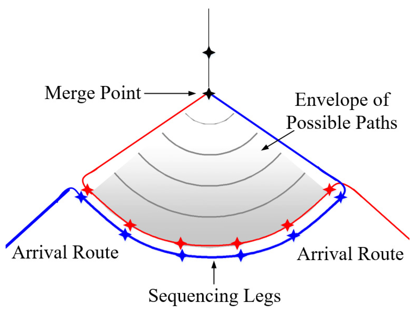
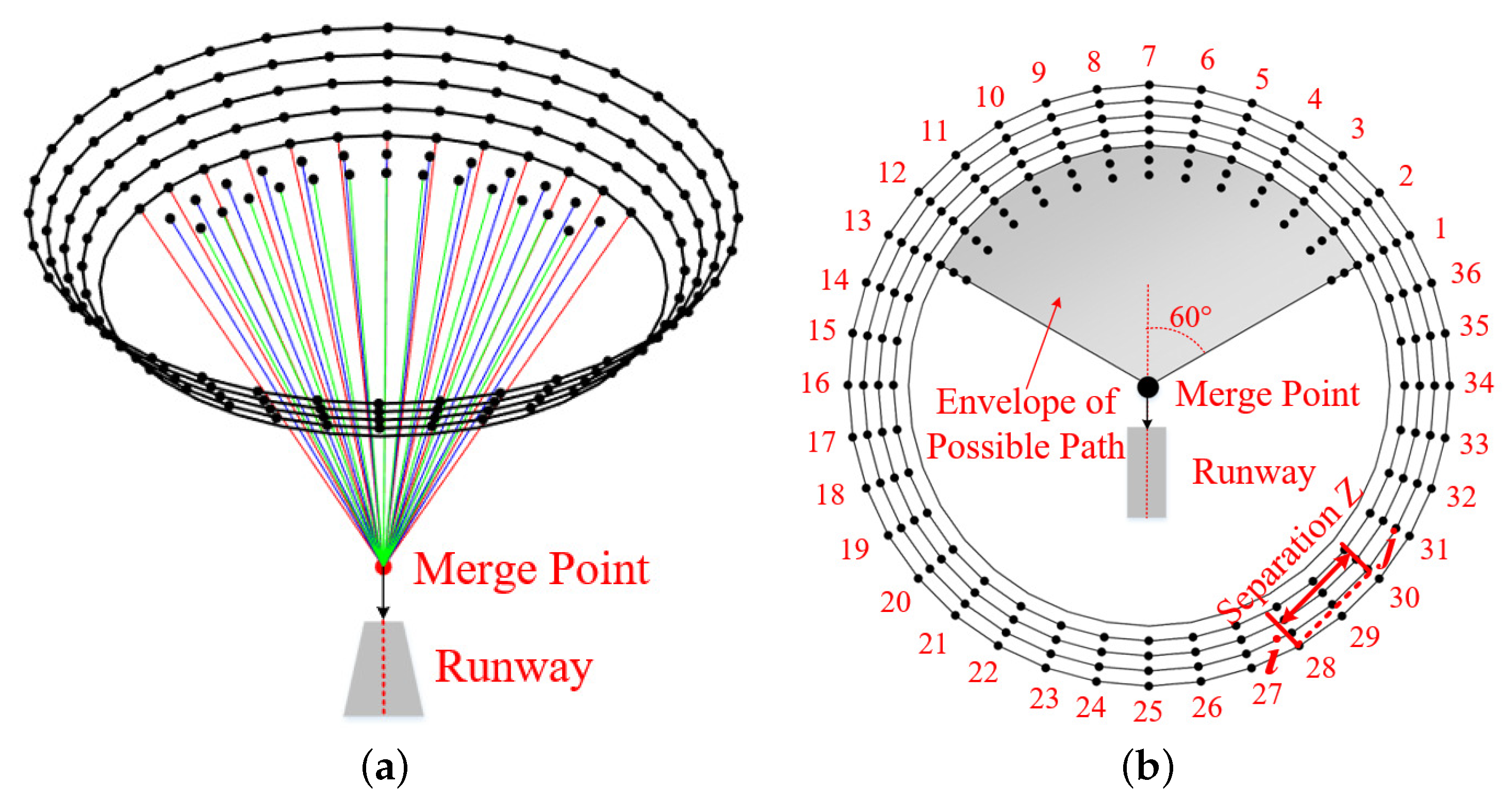
• The design of ICSAA with intuitional operation modes: In order to increase the elasticity of traditional STAR, and the capacity of sequencing legs in the PMS, a flexible terminal airspace called ICSAA was designed to merge traffic streams from all the directions and accommodate more aircraft using circular design. Based on ICSAA, two concise and intuitive operation modes: Mode H and Mode V, were designed to ensure the predictability, safety, and transparency of automated CDO operations.
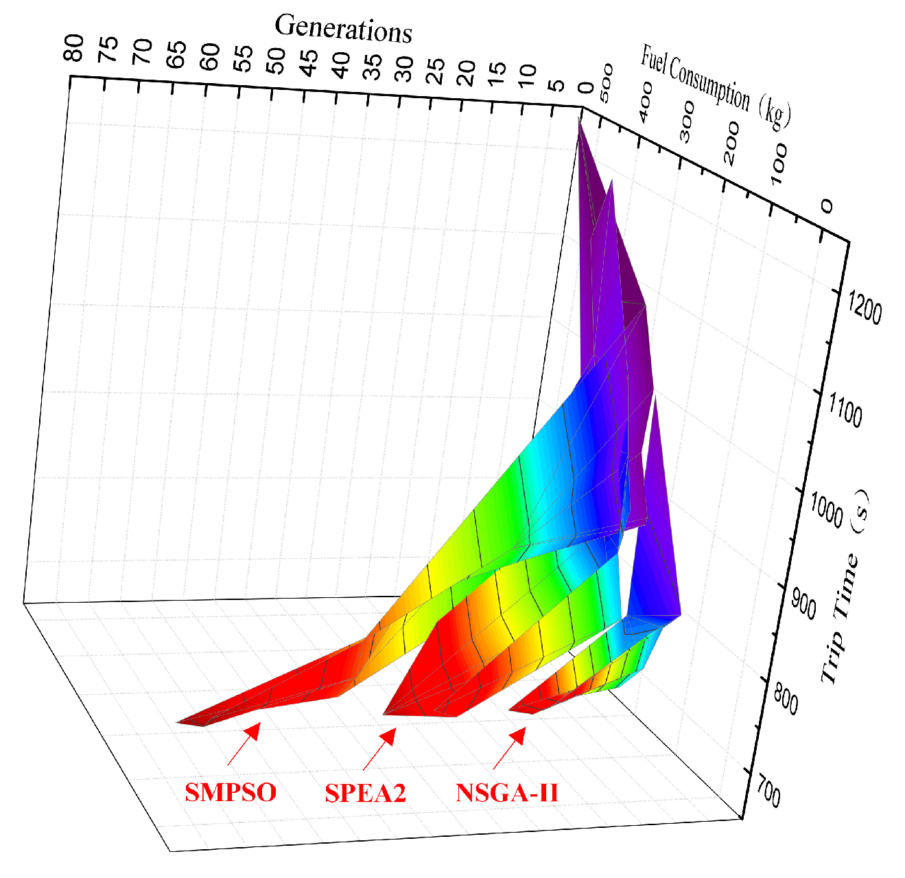
• Pareto optimal front generation for Conflict-free CDO trajectories in the ICSAA: Inside the ICSAA, a multi-objective optimization model that aims at generating conflict-free CDO trajectories with minimal fuel consumption and trip time is proposed by simulating flight dynamics. By comparing with some state-of-the-art multi-objective algorithms, the Non-dominated Sorting Genetic Algorithm with Elitist Strategy (NSGA-II) shows its best performance in convergence near the true Pareto optimal front efficiently, thus is selected to solve the proposed optimization problem.
• Multi-attribute decision-making for optimal CDO trajectories selection: In order to select the optimal trajectories among the Pareto optimal front, from the perspective of both pilots’ and controllers’ preferences, we additionally take collision risk as an attribute besides fuel consumption and trip time. The entropy-based TOPSIS method is adopted to select an unique solution by multi-attribute decision-making strategies. To validate the proposed model and algorithm, the overall performance in single-aircraft, low-density and high-density scenarios are investigated. The results verified that proposed automated CDO trajectory planning in the ICSAA are of high efficiency and strike a better trade-off in terms of economy, efficiency, and safety.

The remainder of this paper is organized as follows: We first illustrate the structure and operational procedures of the ICSAA in Section 2; then, the descriptions are made to explain the detailed trajectory planning problems to be solved in the novel airspace in Section 3. In order to derive optimization objectives, the aircraft performance model and fuel consumption model are established in Section 4 and Section 5, respectively, followed by a multi-objective optimization model in Section 6 and multi-attribute decision-making strategies in Section 7. Section 8 shows the numerical experiments of verifying the effectiveness of proposed methods in different scenarios. Conclusion and the future work are discussed in Section 9.

2. The Novel CDO Airspace Design

2.1. Basic Structure of the Inverted Crown-Shaped Arrival Airspace

According to Doc 9931 Continuous Descent Operation Manual, CDO is an aircraft operating technique aided by appropriate airspace and procedure design and reliable ATC clearances enabling the execution of an optimized trajectories with low engine thrust settings and, where possible, a low drag configuration, thereby reducing fuel burn and emissions during descent. Based on that ideology and enlightened by PMS, we proposed a novel flexible terminal airspace structure and operation procedure, named the ICSAA.

In the ICSAA, we still instruct flights with “direct to” instructions instead of radar vectoring, which could reduce the pilot-ATC communication. Given that the length and number of sequencing legs impose constraints on the performance of the PMS, we extend the arc-shaped sequencing leg to a circle. As shown in Figure 2, we define the artificial terminal area as a series of concentric sequencing rings with the merge point in the center. Each ring has preset waypoints spaced 10° apart from each other along the circumference to ensure safety separation between arriving aircraft. The artificial ICSAA has five levels of rings at different altitude. The altitude of the outermost ring is 6000 m, on which waypoints represent the entry points, while the innermost ring is at 4800 m, on which each waypoint represents the beginning of the CDO trajectory. The vertical separation between adjacent rings is 300 m. It is worth noting that, for the fifth-level ring, there are three layers at the same altitude. Departing from different waypoints on different layers, aircraft could fly to the merge point with different flight path angles ranged from 3° to 4°. In addition, to assure a smooth and efficient interception to the glide slope, the height of the merge point and the central angle of the fan-shaped envelope is set as 900 m and 120°, respectively. For the sake of simplicity, we numbered the waypoints along each ring, as shown in Figure 2b. Please note that, at the fifth level, the waypoints on the outermost layer, the second layer, and the third layer are numbered from 1 to 13, 14–26, and 27–39, respectively.

2.2. The Operational Procedure

Based on flight dynamics of aircraft in the air, two switchable operational modes are defined in the ICSAA: Mode H and Mode V, a multiphase mixed-integer optimal control approach.

Definition 1 (Mode H).

The aircraft is considered as flying into a horizontal plane in a clockwise direction (or anti-clockwise direction). Thus, flight path angle γ, the derivative of flight path angle $\dot{\gamma }$ and the derivative of height $\dot{h}$ are set to 0. In this mode, the equation also holds: $Lcos\varphi =mg$, where L is lift; ϕ is bank angle; m is the mass of aircraft, and g is the gravitational acceleration.

Definition 2 (Mode V).

The aircraft is considered as flying into the vertical plane, performing a leveled-wing descent. Therefore, flight path angle γ, the derivative of flight path angle $\dot{\gamma }$ and the derivative of height $\dot{h}$ are not equal to 0, while the bank angle ϕ is set to 0.

Furthermore, to assure trajectory predictability and operation order, aircraft should descend level by level and cannot go through the interior of ICSAA. In other words, the aircraft must always fly on the wall of the ICSAA. Therefore, we define Separation Z. If and only if the separation Z is less than a certain value, the aircraft could descend with Mode V; otherwise, the aircraft had to fly along the circumference of rings in a clockwise direction (or anti-clockwise direction) with Mode H.

Definition 3 (Separation Z).

Suppose that the present position of aircraft is at the waypoint $i(x_i,y_i,h_i)$, for any waypoint $j(x_j,y_j,h_j)$ on the adjacent inner ring, which the aircraft is going to fly to, theSeparation Zis presented in Figure 2b and defined by $Z(i,j)=\sqrt{{(x_i-x_j)}^2+{(y_i-y_j)}^2}$.

In the multi-aircraft scenario, the situation would be more complex. Not only should Separation Z be less than the certain value but also no potential conflicts exist during descending, when the aircraft could start to fly to the next inner ring. Otherwise, it would fly with Mode H until meeting descent conditions. Obviously, when flying along the circumference of rings, aircraft should keep the safety separation with preceding aircraft by adjusting speed.

Compared with traditional PMS, thanks to the circular design, the ICSAA could integrate inbound flow from all directions, and the sequencing legs (i.e., the rings of ICSAA) would accommodate more aircraft. The proposed intuitive flight modes also possess positive potentials in reducing operational complexity while simplifying automated conflict-free trajectory planning. To some extent, this design also renders more flexible segregation of the inbound and outbound flow. Furthermore, the fifth-level rings provide more continuous descending options for aircraft with different flight path angles, which would significantly affect the fuel consumption and trip time. Therefore, the proposed ICSAA has higher structural and procedural flexibility that would provide larger solution space for CDO trajectory optimization.

3. Problem Definition

In order to search optimal CDO trajectories, the airspace is modeled as a network $G=(V,E)$, and each vertex $(i,j)$ represents waypoint of ICSAA. The adjacency matrix is constructed, of which the element, $\mathsf{\Theta }=e[(i_n,j_n),(i_m,j_m)]$, represents connectivity of the directed network, in accordance with the operation rules of ICSAA mentioned above. If the edge, $(i_n,j_n)\to (i_m,j_m)$, is connected, $e[(i_n,j_n),(i_m,j_m)]=1$; otherwise, $e[(i_n,j_n),(i_m,j_m)]=+\propto$. Therefore, the path $P_{ath}$ of the aircraft $\alpha$ is expressed as a set of connected vertices in network G. The problem we studied can be stated as follows: based on the expected entry points and expected arrival time of aircraft, we would generate optimal CDO trajectories automatically in the ICSAA, aiming at achieving best performance in economy, efficiency, and safety on the promises of acceptable computation time, to support the pre-tactic operation of air traffic management.

4. Aircraft Performance Model

Aircraft performance model is used to control the flight dynamics in accordance with the flight modes in the ICSAA. Glover and Lygeros [25] came up with the Point Mass Model (PMM), derived from the Newtonian dynamics. EUROCONTROL [26] proposed the Total-Energy Model (TEM) in Base of Aircraft Data (BADA), derived from the work-energy theorem for continuous descent. In this research, in order to simplify the trajectory optimization problem, a Point-Mass performance model, adapted from the work mentioned above, is adopted to simulate the CDO flight while measuring the fuel consumption and trip time. The model can be stated as follows:

$$\begin{array}{cc}\hfill \dot{x}& =vcos\psi cos\gamma +{\omega }_1\hfill \\ \hfill \dot{y}& =vsin\psi cos\gamma +{\omega }_2\hfill \\ \hfill \dot{z}& =vsin\gamma +{\omega }_3\hfill \\ \hfill \dot{v}& =\frac{1}{m}(Tcos\tau -D-mgsin\gamma )\hfill \\ \hfill \dot{\psi }& =\frac{1}{mv}(L+Tsin\tau )sin\varphi \hfill \\ \hfill \dot{\gamma }& =\frac{1}{mv}(L+Tsin\tau )cos\varphi -mgcos\gamma )\hfill \end{array},$$

(1)

where the dotted terms are derivatives with respect to time; x, y, and h represent the position of aircraft in the three-dimension coordinate system; v is true airspeed; $\varphi$ is bank angle; $\tau$ is attack angle; $\gamma$ is flight path angle; $\psi$ is course angle; $W=({\omega }_1,{\omega }_2,{\omega }_3)\in R^3$ is wind speed; T is engine thrust; D and L is the aerodynamic drag and lift, which are modeled, respectively, as:

$$\begin{array}{cc}\hfill D& =\frac{C_D·\rho ·v^2·S}{2}\hfill \\ \hfill L& =\frac{C_L·\rho ·v^2·S}{2}\hfill \end{array},$$

(2)

where $\rho$ is air density; S is the wing reference area; and $C_D$ and $C_L$ are the drag coefficient and the lift coefficient, respectively, modeled as:

$$\begin{array}{cc}\hfill C_D& =C_{D0}+C_{D2}\times C_L^2\hfill \\ \hfill C_L& =\frac{2mg}{\rho ·v^2·S·cos\varphi }\hfill \end{array},$$

(3)

where $C_{D0}$ and $C_{D2}$ are BADA coefficients. The drag coefficient $C_D$ is expressed as a function of the lift coefficient $C_L$.

When simulating the aircraft descent, we use the standard speed profile recommended by BADA and perform curve fitting for those data, as shown in Figure 3. The goodness of curve fitting $R^2$ = 0.9820. The result is stated as follows:

$$v(h)=-1.943\times {10}^{-6}·h^2+0.03499·h+73.34.$$

(4)

In the above expressions, velocity is the function of height. In order to obtain the derivative of velocity versus time, we made the following deformations.

$$a=\frac{dv}{dt}=\frac{dv}{dh}·\frac{dh}{dt}.$$

(5)

It is worth noting that, in order to improve the accuracy of the flight descent path modeling, some atmospheric properties (temperature, pressure, density) are expressed as a function of altitude, based on the BADA reversion 3.11 issued in 2013, rather than fixed values [27].

$$\begin{array}{cc}\hfill \rho & =\frac{p}{R·T_{em}}\hfill \\ \hfill T_{em}& =T_{em,0}+▽T_{em}+\beta \ast h\hfill \\ \hfill p& =p_0·{(\frac{T_{em}-▽T_{em}}{T_{em,0}})}^{-\frac{g}{\beta ·R}}\hfill \end{array},$$

(6)

where R is real gas constant for air, the value of which is 287.05287 m²/(K · s²); $T_{em,0}$ is the standard atmospheric temperature at mean sea level, of which the value is 288.15 K; $▽T_{em}$ is temperature differential at mean sea level, which is the difference in atmospheric temperature at mean sea level between a given non-standard atmosphere and International Standard Atmosphere (ISA), and the value is set to 0; $\beta$ is ISA temperature gradient with altitude below the tropopause, the value of which is −0.0065 K/m; $p_0$ is standard atmospheric pressure at mean sea level; and g is gravitational acceleration, the value of which is 9.80665 m/s².

Based on the aircraft performance model (those equations are denoted as M), once the starting point $(i_s,j_s)$, ending point $(i_e,j_e)$, flight path $P_{ath}$, and initial speed $v_0$ are determined, the real-time position of aircraft $(x,y,h)$ at time t could be obtained following speed-altitude profile recommended by BADA, which can be expressed by the Equation (7). Such an equation enables the conflict detection of CDO trajectories.

$$H(t,(i_s,j_s),(i_e,j_e),P_{ath},v_0,M)=(x,y,h).$$

(7)

5. Fuel Consumption Model

Thrust Specific Fuel Consumption (TSFC) model in BADA is applied for fuel consumption computation. For the jet engines, the thrust specific fuel consumption is specified as a function of the true airspeed:

$$\begin{array}{cc}\hfill \eta & =C_{f1}\times \left(1+\frac{v}{C_{f2}}\right)\hfill \\ \hfill f_c& =T\times C_{fcr}\times \eta \hfill \\ \hfill F_c& ={\int }_0^{T_{ime}}{f}_{c}dt\hfill \end{array},$$

(8)

where $C_{f1}$, $C_{f2}$ are the fuel flow coefficient, and $C_{fcr}$ is the fuel flow correction factor, the value of which are given by BADA; $f_c$ is the fuel flow and the fuel consumption, and $F_c$ is the integral of fuel flow with respect to time. In the network of ICSAA, the integral can be also approximately considered as a sum of discretized fuel consumption on each link along the whole flight path.

6. Optimization Function Formulation

6.1. Decision Variables

In order to identify whether the aircraft $\alpha$ fly through the $j_{th}$ waypint of the $i_{th}$ ring in the ICSAA, the 0-1 variable, $\chi {(\alpha )}_{(i,j)}$, is introduced, as shown in Formula (9):

$$\chi {(\alpha )}_{(i,j)}=\left\{\begin{array}{cc}1,\hfill & aircraft \alpha fly by waypoint(i,j)\\ 0,\hfill & otherwise\end{array}.\right.$$

(9)

Furthermore, in order to indicate the connectivity among nodes determined by Formula (9), a variable is introduced to denote whether the aircraft chooses the edge between two nodes as a part of the CDO path. Assume two nodes are $(i_1,j_1)$ and $(i_2,j_2)$, respectively,

$$\mu {(\alpha )}_{(i_1,j_1)}^{(i_2,j_2)}=\left\{\begin{array}{cc}1,\hfill & aircraft \alpha fly by (i_1,j_1)\to (i_2,j_2)\\ 0,\hfill & otherwise\end{array}.\right.$$

(10)

6.2. Objectives

Total fuel consumption and trip time that aircraft take from entry point to Final Approach Fix (FAF) are set as two objectives for the CDO trajectory optimization. Please note that the noise abatement here is not chosen as an objective in an artificial scenario because the noise impact evaluation highly relies on the geographical features of the vicinity of airport [28].

$$min\{\sum _{\alpha }\sum _i\sum _{j}f{(\alpha )}_{(i,j)}^{\mathbb{N}(i,j)}\mu {(\alpha )}_{(i,j)}^{\mathbb{N}(i,j)},\sum _{\alpha }\sum _i\sum _{j}t{(\alpha )}_{(i,j)}^{\mathbb{N}(i,j)}\mu {(\alpha )}_{(i,j)}^{\mathbb{N}(i,j)}\},$$

(11)

where $\alpha$ names different aircraft; $f(\alpha )$ and $t(\alpha )$ are the fuel consumption and trip time, which aircraft $\alpha$ spent during flight from entry point to the FAF; and $\mathbb{N}(i,j)$ is introduced to represent the next waypoint connects with waypoint $(i,j)$ in the planed CDO trajectory.

6.3. Constraints

• Uniqueness Constraints
  The trajectory of aircraft $\alpha$ should be unique and definite, that is, for any vertex $(i_p,j_p)$ along a trajectory, one and only one following waypoint directly connects to it.

  $$\sum _i\sum _j\mu {(\alpha )}_{(i_p,j_p)}^{(i,j)}=1,(i_p,j_p)\in \left\{(i,j)\right|\chi {(\alpha )}_{(i,j)}=1\}.$$

  (12)
• Descent Constraints
  In order to assure that aircraft could descend level by level, thus, the sum of $\chi {(\alpha )}_{(i,j)}$ in the each level should be equal to or greater than 1.

  $$\sum _j\chi {(\alpha )}_{(i,j)}\ge 1,i\in \{1,2,3,4,5\}.$$

  (13)
• Connection Constraints
  The trajectory of each aircraft should be in compliance with operation mode of ICSAA mentioned above. The edge $[(i,j),\mathbb{N}(i,j)]$ along the planned trajectory shall satisfy that

  $$e[(i,j),\mathbb{N}(i,j)]=1.$$

  (14)
• Acceleration Rate
  The accelerate rate is a value that relates to the performance of aircraft. In general, in view of the comfort for passengers, the accelerate rate could not be too large. The BADA manual recommends a maximum longitudinal acceleration:

  $$a_{(i,j)}^{\alpha }\le 0.6096 {\mathrm{m}/\mathrm{s}}^2.$$

  (15)
• Final Approach Speed
  When aircraft start to land, the velocity should be decreased to intercept the glide slope. But there is a minimum speed limit. The minimum landing speed $v_{min}$ is now determined as follows:

  $$v_{MergePoint}^{\alpha }\ge 1.3\times v_{stall}\sqrt{\frac{m_{MergePoint}^{\alpha }}{m_{ref}^{\alpha }}}+10,$$

  (16)

  where 1.3 is a factor recommended by the BADA manual for all aircraft operations, $v_{stall}$ is the stall speed at the reference mass $m_{ref}$, and m is the simulated aircraft mass which is updated with fuel consumption.
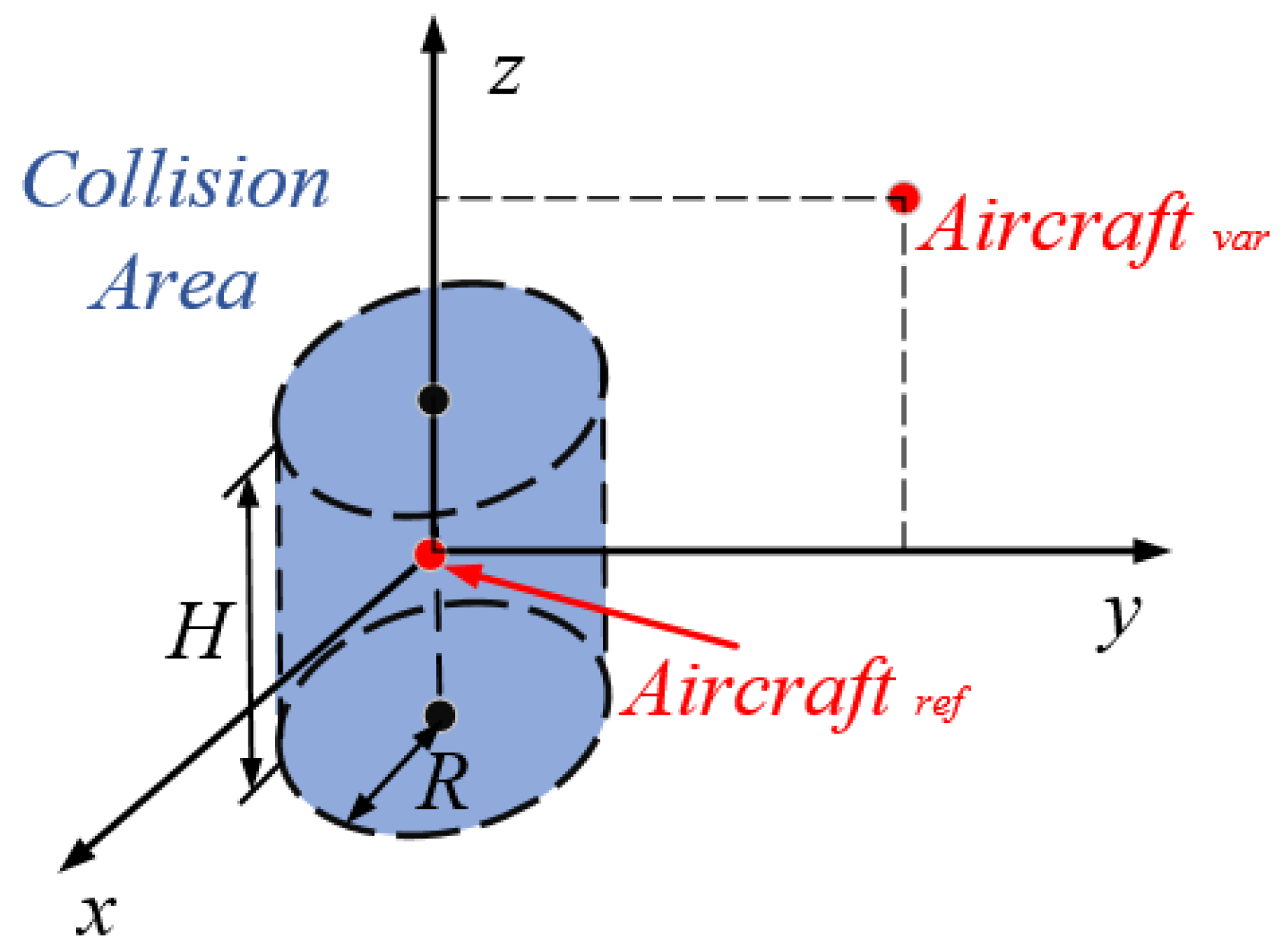
• Safety Separations
  In order to assure safety, the separation between aircraft shall be larger than the minimum. The position of aircraft ${\alpha }_1$ and aircraft ${\alpha }_2$ at time t could be obtained with the Equation (7), then we could get the horizontal separation at time t, $S_{hor}(t,{\alpha }_1,{\alpha }_2)=\sqrt{{(x_{{\alpha }_1}-x_{{\alpha }_2})}^2+{(y_{{\alpha }_1}-y_{{\alpha }_2})}^2}$, the vertical separation $S_{ver}(t,{\alpha }_1,{\alpha }_2)=\sqrt{{(h_{{\alpha }_1}-h_{{\alpha }_2})}^2}$. According to regulation, two aircraft are considered to be in a conflict if their horizontal separation is less than 10 km and vertical separation is less than 300 m. Therefore, during approach, $C(t,{\alpha }_1,{\alpha }_2)$ should always be 1.

  $$C(t,{\alpha }_1,{\alpha }_2)=\left\{\begin{array}{cc}0& S_{hor}\le 10km\wedge S_{ver}\le 300m\\ 1& others\end{array}.\right.$$

  (17)

6.4. Solution Algorithm for Generating Pareto Optimal Front

In order to solve the multi-objective optimization problem, we introduce the Non-dominated Sorting Genetic Algorithm with Elitist Strategy (NSGA-II) algorithm, which has the best performance for this particular problem, compared with the state-of-the-art multi-objective optimization algorithms, as illustrated in Section 8.2. Adaptions to the critical genetic operators are made to generate the Pareto solutions [29,30]. The framework of the NSGA-II algorithm is illustrated in Figure 4.

• Coding and Decoding Schema
  Considering the integrity and accuracy of trajectory planning, we will code all the directed edges of ICSAA, (i.e., $e[(i_n,j_n),(i_m,j_m)]=1$), with binary coding schema. Thus, for one aircraft, the chromosome composed of decision variables is denoted as $X(\alpha )=\{\mu {(\alpha )}_{(1,1)}^{(1,2)},\mu {(\alpha )}_{(1,1)}^{(2,1)},\mu {(\alpha )}_{(1,1)}^{(2,2)},\mu {(\alpha )}_{(1,1)}^{(2,3)},\mu {(\alpha )}_{(1,1)}^{(2,4)},...\mu {(\alpha )}_{(5,39)}^{Merge\hspace{1em}Point}\}$, while, in the multi-aircraft scenario, the chromosome is the splicing of chromosome for the each aircraft, that is, $C_h=\{X({\alpha }_1),X({\alpha }_2),X({\alpha }_3),\cdots ,X({\alpha }_n),F,T_{ime},r,D_{cro}\}$, where F and $T_{ime}$ are the fitness of the individual, defined as the reciprocal of objective functions, and r and $D_{cro}$ are the rank and crowding distance, respectively, which can be calculated based on Non-Dominated Sort introduced in the following part. Based on above coding schema, we can easily decode the chromosome into a trajectory of aircraft $\alpha$.
• Initial Population
  Initial population is the starting state of iteration for heuristic algorithm, which has a great effect on optimized results and computational efficiency. In the single aircraft scenario, the trajectory is optimized with a randomly generated initial population, while, in the multi-aircraft scenario, the initial population is generated by randomly combining the non-determined solutions derived in the single aircraft scenario.
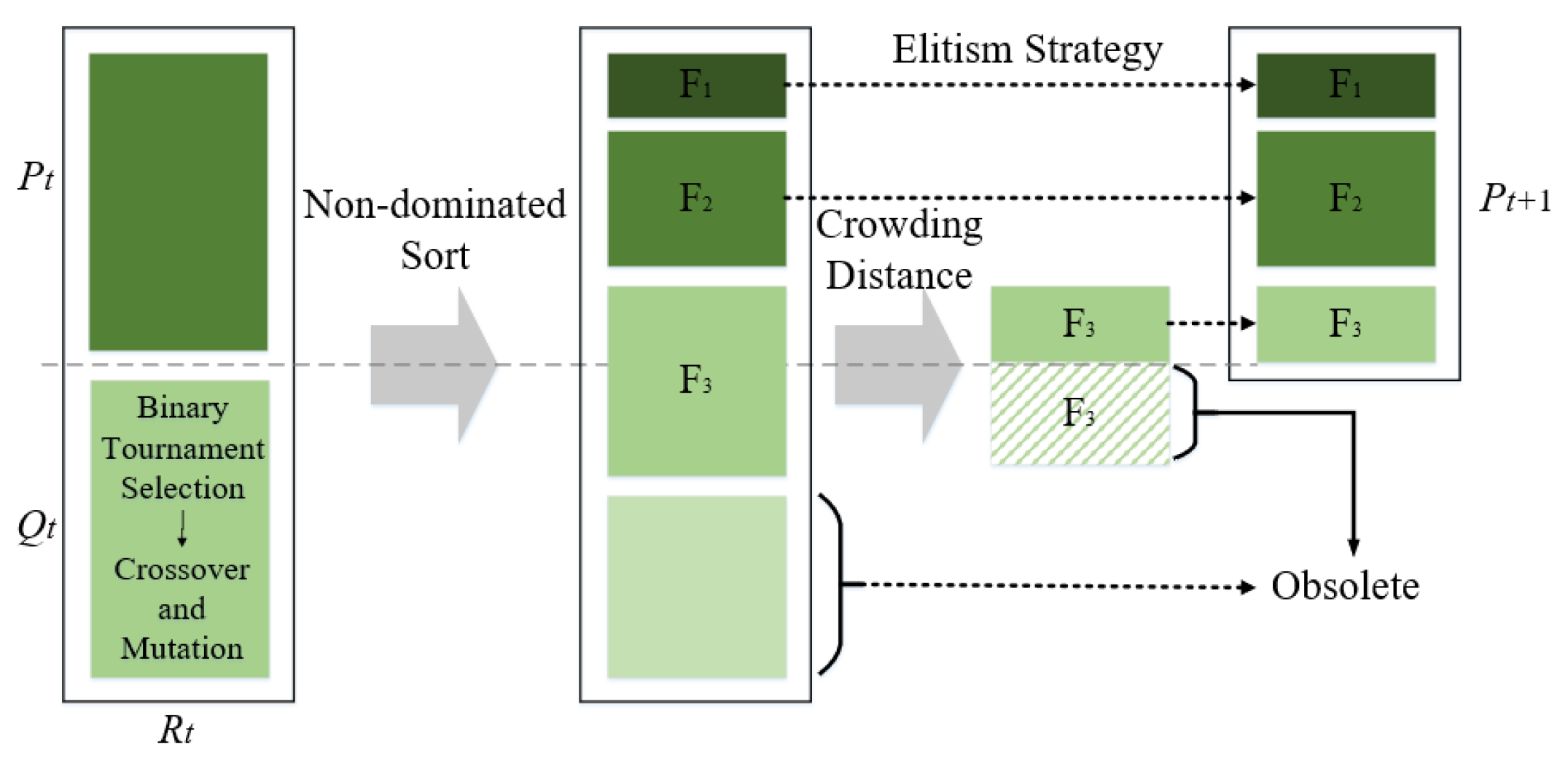
• Non-Dominated Sort and Crowding Distance
  Each chromosome of the NSGA-II corresponds to a feasible solution, by which we could get the trajectory of the aircraft inside the ICSAA through decoding. The population, composed of multiple chromosomes, is the set of feasible solutions. Based on the objective function, we could get the value of fuel consumption and trip time for each solution, as well as the fitness of the chromosomes. In order to achieve faster convergence, each population can be layered and sorted to create multiple Pareto fronts with different rankings based on fitness. Solutions with lower rankings (higher fitness) are preferred. If any two solutions belong to the same front, then the solution located in a less crowded region is regarded as a better one, by introducing crowding distance mechanism to improve diversity of the population. Obviously, solutions with larger crowding distance imply that there would be probably more unexplored solution space around them. Determined by aforementioned non-domination sort and crowding distance, the identified prospective individuals will be moved to the front of population and used to generate the next generation.
• Genetic Operations
  In this research, the elite individual is selected with binary tournament selection and elitism strategy to create the offspring with crossover and mutation. To be specific, the crossover operator is implemented pairwise. The basic unit of crossover is the gene fragment, which could represent an entire trajectory of the aircraft. Suppose we pick out two individuals $C_{h,1}$ and $C_{h,2}$ in the current population randomly; then, two new individuals will be generated in the following way:

  $$\begin{array}{cc}\hfill C_{h,1}=\{X{({\alpha }_1)}_1\cdots X{({\alpha }_{rp})}_1,\cdots ,X{({\alpha }_n)}_1,\cdots \}& \to C_{h,1}^{\prime }=\{X{({\alpha }_1)}_1\cdots X{({\alpha }_{rp})}_2,\cdots ,X{({\alpha }_n)}_1,\cdots \}\hfill \\ \hfill C_{h,2}=\{X{({\alpha }_1)}_2,\cdots X{({\alpha }_{rp})}_2,\cdots ,X{({\alpha }_n)}_2,\cdots \}& \to C_{h,2}^{\prime }=\{X{({\alpha }_1)}_2,\cdots X{({\alpha }_{rp})}_1,\cdots ,X{({\alpha }_n)}_2,\cdots \}\hfill \end{array},$$

  (18)

  where $rp$ is a random integer between 1 and n. The above crossover operation is triggered by a crossover probability.
  Mutation is operated in a simple and intuitive way. For each of individuals, once the random number is greater than the mutation probability that we set beforehand, the individual starts to mutate at a selected gene randomly. After the mutation process, if the individual does not satisfy the constraints mentioned above, the fitness of the individual will be set to 0 and the individual would be rejected automatically during solution. After the process of crossover and mutation, combine the newly generated population and parent population, and calculate fitness value of each chromosome. Use elite strategy to keep the better chromosome to generate a new population.
• Termination Conditions
  By setting the maximum number of iteration and test the convergence results of each generation population, we could terminate the heuristic algorithm. In this article, if the number of elements in the Pareto front account for 80 percent or greater, of the population size, the heuristic algorithm terminated. Otherwise, the algorithm could terminate when reaching the maximum number of iterations.

7. Optimal Trajectory Election Using Multi-Attribute Decision Making (OTE-MADM)

Based on the Pareto optimal fronts obtained by the NSGA-II algorithm, determining a unique solution from the Pareto optimal fronts is a crux in the application of the CDO. Thus, we assess each solution of Pareto front set with entropy-based TOPSIS method [31,32].

7.1. Attributes

The economy, efficiency, and safety metrics shall be considered in trajectory planing, which represent common interests among different stakeholders (e.g., pilots, ATC, airlines). Here, although the safety separation between aircraft is guaranteed during trajectory planning, with the consideration of uncertainty factors (e.g., positioning error) in real-world operation, we introduce the collision probability as an additional index to evaluate the potential risks and operational robustness of planned CDO trajectories. It is worth noting that there is no collision in the single-aircraft scenario (refer to Section 8.2), so the collision probability will not be included.

Collision probability is determined by the co-variance matrices of the position errors, shape and track of aircraft [33]. The position vector of aircraft could be obtained by the aircraft performance model, while the position error vector is usually obtained by the prediction error. Assume there are two aircraft ${\alpha }_1$ and ${\alpha }_2$ in the airspace, the real-time positions of them are denoted as $(x_{\alpha 1},y_{\alpha 1},h_{\alpha 1})$ and $(x_{\alpha 2},y_{\alpha 2},h_{\alpha 2})$, respectively. If the probability density function of collision is $f_{ca}$, the calculation of collision probability can be transformed into an integral of the probability density function of the equivalent region, $V_{area}$. The formulation is shown as follows:

$$P_{ca}={\int \int \int }_{V_{area}}{f}_{ca}(x_{\alpha 1},y_{\alpha 1},h_{\alpha 1},x_{\alpha 2},y_{\alpha 2},h_{\alpha 2})dv.$$

(19)

For each pair of aircraft, one is regarded as a reference aircraft, the other is an intruder one. When calculating collision probability, we assume the following conditions for simplicity:

• The position error of aircraft satisfies the Gauss distribution.
• The co-variance matrices of aircraft positions are not related. For each pair, the position error of the reference aircraft is $e_r$, while the position error of the intruder is $e_v$, and the relative position error of them is $e_f=e_r+e_v$. Based on position error, the co-variance matrix of the relative random error of two aircraft is expressed as a diagonal matrix:

  $$C_{ov}=\left[\begin{array}{ccc}{\sigma }_x^2& 0& 0\\ 0& {\sigma }_y^2& 0\\ 0& 0& {\sigma }_z^2\end{array}\right].$$

  (20)

Based on such assumptions, the intruder is regarded as a point and takes the center of the reference aircraft as the origin of the coordinate system, so the collision area of them regarded as a cylinder with height of $\mathbb{H}$ and radius of $\mathbb{R}$, where $\mathbb{H}$ is the sum of their height, and $\mathbb{R}$ is the sum of radius of their envelop, as shown in Figure 5. The relative position of the intruder is $({\mu }_x,{\mu }_y)$ in the horizontal plane, so the probability density function, $f_{ca,XY}(x,y)$, and collision probability, $P_{ca,XY}$, are:

$$\begin{array}{cc}\hfill f_{ca,XY}(x,y)& =\frac{1}{2\pi {\sigma }_x{\sigma }_y}exp[-\frac{1}{2}(\frac{(x-{\mu }_x^2)}{{\sigma }_x^2}+\frac{(x-{\mu }_y^2)}{{\sigma }_y^2})],\hfill \end{array}$$

(21)

$$\begin{array}{cc}\hfill P_{ca,XY}& ={\int \int }_{x^2+y^2\le {\mathbb{R}}^2}{f}_{ca,XY}(x,y)dxdy.\hfill \end{array}$$

(22)

In order to calculate the collision probability in two-dimensional space, a fast computation method based on compressed infinite series is applied to solve the problem of the probability integration. After derivation, the upper form is rewritten as follows [33]:

$$P_{ca,XY}=exp[-\frac{1}{2}(\frac{{\mu }_x^2}{{\sigma }_x^2}+\frac{{\mu }_y^2}{{\sigma }_y^2})][1-exp(-\frac{{\mathbb{R}}^2}{2{\sigma }_x{\sigma }_y})],$$

(23)

where ${\sigma }_x$ and ${\sigma }_y$ are the variance of the probability density function.

Similarly, the relative position of the intruder aircraft is ${\mu }_z$ in the vertical plane, so the probability density function $f_{ca,Z}(z)$ and collision probability $P_{ca,Z}$ are:

$$\begin{array}{cc}\hfill f_{ca,Z}(z)& =\frac{1}{\sqrt{2\pi }{\sigma }_z}exp[-\frac{{(z-{\mu }_z)}^2}{2{\sigma }_z^2}],\hfill \end{array}$$

(24)

$$\begin{array}{cc}\hfill P_{ca,Z}& ={\int }_{-\frac{\mathbb{H}}{2}\le z\le \frac{\mathbb{H}}{2}}{f}_{ca,Z}(z)dz.\hfill \end{array}$$

(25)

According to the functional nature of normal distribution, we find a rational function, in which the function characteristic is consistent with that of distribution function, and its derivative characteristic is consistent with probability density function of normal distribution. The rational function is:

$$P_{ca,Z}=\frac{exp[C_{ca,Z}(z-{\mu }_z)]}{1+exp[C_{ca,Z}(z-{\mu }_z)]},$$

(26)

where $C_{ca,Z}=\frac{4}{\sqrt{2\pi }{\sigma }_z}$, and ${\sigma }_z$ is the variance of the probability density function.

7.2. Entropy-Weights Method

In MADM, whether weights of attributes (i.e., fuel consumption, trip time, and collision probability) are reasonable or not is critical to the decision-making accuracy. Entropy Weight Method (EWM) is an important information weight model that has been extensively studied and practiced. Compared with various subjective weighting models, the most significant advantage of the EWM is the avoidance of the interference of human factors on the weight of indicators, thus enhancing the objectivity of the comprehensive evaluation results. Therefore, the EWM has been widely used in multi-criteria decision-making [34,35]. Recently, the benefits of the EWM for multi-objective optimization has been also proven [36], although the results are prone to distortion when too many zero values are in the measured indicators [37]. Considering the non-zero features of fuel consumption, trip time, and collision probability, EWM is chosen to calculate the weights of attributes in Pareto’s solutions.

Suppose there are m solutions in the Pareto optimal front; each solution is evaluated with respect to n attributes, i.e., fuel consumption, trip time, and collision probability, in which values constitute a decision matrix $Z={(z_{ij})}_{m\times n}$. Since such attributes in this paper belong to cost value, we normalize each attribute value $z_{ij}$ in decision matrix into a corresponding element $r_{ij}$ with the formulas: $r_{ij}=\frac{ma{x}_i(z_{ij})-z_{ij}}{ma{x}_i(z_{ij})-mi{n}_i(z_{ij})}$, to facilitate inter-attribute comparisons. Note that, among classic normalization methods, the minmax standardization method was validated to be a better option [38,39,40]. The normalized decision matrix is denoted as:

$$R_{m\times n}=\left[\begin{array}{cccc}{r}_{11}& r_{12}& \cdots & r_{1n}\\ r_{21}& r_{22}& \cdots & r_{2n}\\ ⋮& ⋮& \ddots & ⋮\\ r_{m1}& r_{m2}& \cdots & r_{mn}\end{array}\right].$$

(27)

Therefore, entropy and weight of each attribute are formulated as:

$$\begin{array}{cc}\hfill E_j& =-\frac{1}{lnm}\sum _{i=1}^m(P_{ij}·ln{P}_{ij}),\hfill \end{array}$$

(28)

$$\begin{array}{cc}\hfill w_j& =\frac{1-E_j}{n-{\sum }_{j=1}^n(E_j)},\hfill \end{array}$$

(29)

where $P_{ij}=\frac{r_{ij}}{{\sum }_{i=1}^m{r}_{ij}}$, if $r_{ij}=0$, $P_{ij}·ln{P}_{ij}=0$.

7.3. TOPSIS Method

According to the multi-criteria method selection strategy proposed by Wątróbski [31], TOPSIS proposed by Hwang and Yoon, in 1981 [41], was proven to be the most suitable one for this particular decision situation, where the weight of individual criteria has to be considered quantitatively and complete ranking is required. The principle of this method is to rank the alternatives by calculating the distance of each alternative from the positive ideal solution and the negative ideal solution for problems in decision-making, thus determining the optimum alternative. By applying the weights calculated by EWM, entropy-based TOPSIS is adopted to select the optimal CDO trajectories.

As mentioned above, in this paper, we suppose a decision matrix $Z={(z_{ij})}_{m\times n}$, where there are m solutions with n attributes, i.e., fuel consumption, trip time, and collision probability. The TOPSIS method consists of the following steps:

• Normalize the decision matrix. Given that all the attributes of each solution, i.e., fuel consumption, trip time, and collision probability, are cost attributes in the MADM problems, we introduce the following formulas [41] to normalize each attribute value $z_{ij}$ in decision matrix $Z={(z_{ij})}_{m\times n}$ into a corresponding element $u_{ij}$: $u_{ij}=1-\frac{z_{ij}}{\sqrt{{\sum }_{i=1}^m{(z_{ij})}^2}}$.

  $$U_{m\times n}=\left[\begin{array}{cccc}{u}_{11}& u_{12}& \cdots & u_{1n}\\ u_{21}& u_{22}& \cdots & u_{2n}\\ ⋮& ⋮& \ddots & ⋮\\ u_{m1}& u_{m2}& \cdots & u_{mn}\end{array}\right].$$

  (30)
• Calculate the weighted normalized decision matrix. Suppose that weights of attributes, $W={(w_1,w_2,w_3,\cdots ,w_n)}^T$, is obtained with Equation (28), where $w_j\ge 0$, ${\sum }_{j=1}^n{w}_j=1$, we can construct the weighted normalized decision matrix as

  $$K={(w_j{u}_{ij})}_{m\times n}={(k_{ij})}_{m\times n}=\left[\begin{array}{cccc}{k}_{11}& k_{12}& \cdots & k_{1n}\\ k_{21}& k_{22}& \cdots & k_{2n}\\ ⋮& ⋮& \ddots & ⋮\\ k_{m1}& k_{m2}& \cdots & k_{mn}\end{array}\right].$$

  (31)
• Determine the positive and negative ideal solutions. The Positive Ideal Solution (PIS) $A^{+}$ and the Negative Ideal Solution (NIS) $A^{-}$ are determined, respectively, as follows:

  $$\begin{array}{cc}\hfill A^{+}& =\{k_1^{+},k_2^{+}\cdots k_n^{+}\}\hfill \\ \hfill A^{-}& =\{k_1^{-},k_2^{-}\cdots k_n^{-}\}\hfill \end{array},$$

  (32)

  where $k_j^{+}=ma{x}_{1\le i\le m}\left\{k_{ij}\right\}$, and $y_j^{-}=mi{n}_{1\le i\le m}\left\{k_{ij}\right\}$.
• Measure the distance from each solution to PIS and NIS. The separation, $S_i^{+}$ and $S_i^{+}$, are given as:

  $$\begin{array}{cc}\hfill S_i^{+}& =\sqrt{{\sum }_{j=1}^n{(k_{ij}-k_j^{+})}^2}\hfill \\ \hfill S_i^{-}& =\sqrt{{\sum }_{j=1}^n{(k_{ij}-k_j^{-})}^2}\hfill \end{array}.$$

  (33)
• Calculate the closeness coefficient to the ideal solutions. The closeness coefficient of the $i_{th}$ solution in the Pareto optimal front with respect to the ideal solutions, $C_i$, is defined as:

  $$C_i=\frac{S_i^{-}}{S_i^{+}+S_i^{-}}.$$

  (34)
• Rank the preference order. The solutions of the Pareto optimal front can be ranked according to the descending order of $C_i$; the larger $C_i$ means the better solution.

8. Numerical Tests

In this section, numerical results with different settings of (user-defined) algorithm parameters and various scenarios were presented and discussed to validate the performance of proposed trajectory optimization method in the new airspace. The overall process is run on a 2.00 GHz, CORE i7 CPU, under Windows 10 operating system laptop based on MATLAB code.

8.1. Parameter Setting

For simplification, we assume the geopotential pressure altitude is equal to geodetic altitude; true airspeed is equal to ground speed, which implies the international standard atmosphere and no wind. Airbus A320, one of main aircraft types in the aviation industry, is selected as specific aircraft for the CDO trajectory optimization in the experiments. Performance parameters of A320 in BADA version 3.9 are presented in

Table 1. Basic parameter of A320.

Performance Parameter	Value
reference mass (kg)	64,000
surface area of wing (m2)	122.6
$C_{f1}$	0.6333
$C_{f2}$	859.03
$C_{fcr}$	0.95423

.

8.2. Algorithm Comparison

In order to verify the superiority of NSGA-II in solving proposed trajectory planning problem, two kinds of multi-objective optimization algorithms with good performance and wide application at present [30] have been selected: Speed-constrained Multi-objective Particle Swarm Optimization (SMPSO) and Improving the Strength Pareto Evolutionary Algorithm (SPEA2). Based on the two-dimensional objective function space where the fuel consumption and flight time are taken as the coordinate axes, five evaluation indexes are used to comprehensively demonstrate the performance of algorithms: general distance (GD), inverted generational distance (IGD), hypervolume (HV), Spacing, and maximum Pareto front error (MPFE) [30]. In order to compare the performance characteristics of NSGA-II, SMPSO, and SPEA2 algorithms in different problem scales, three traffic scenarios with different densities, i.e., 1/6/12 aircraft arrive at the entry points simultaneously, are designed. In order to enhance the comparability, the three algorithms have the same convergence conditions. Moreover, the population number of NSGA-II and SPEA2 is 2000, the maximum number of iterations is 80, the crossover probability is 0.3, and the mutation probability is 0.7; in SMPSO, the number of particles and archive size is 2000, and the maximum number of iterations is 80, as well. The parameters corresponding to the optimal solution performance are set as follows: initial velocity influence factor is 0.2, individual optimal influence factor is 0.2, and global optimal influence factor is 0.5. Under the above benchmark parameters, the performance of the three algorithms is shown in

Table 2. The comparison of performance of three different algorithms.

	1 Aircraft			6 Aircraft			12 Aircraft
	NSGA-II	SPEA2	SMPSO	NSGA-II	SPEA2	SMPSO	NSGA-II	SPEA2	SMPSO
GD	0.0104	0.0150	0.0159	0.0255	0.026	0.0259	0.0412	0.0533	0.0483
IGD	0.1385	0.1994	0.4233	0.1787	0.2307	0.5237	0.2136	0.2593	0.4233
HV	1.1810	1.0192	0.9999	1.4517	1.0353	1.2359	1.8325	1.2543	1.5786
Spacing	0.0694	0.0758	0.0828	0.0746	0.0784	0.0988	0.0743	0.0824	0.0988
MPFE	1.2274	1.4045	1.4019	1.5743	1.639	1.6319	1.6432	1.9043	1.8377

.

The results show that, although the performance of the three algorithms decreases with the increase of the problem size, NSGA-II is always better than the other two algorithms in various performance indicators. In addition, taking the single-aircraft scenario as an example, the convergence rate of NSGA-II is obviously better than the other two algorithms, as shown in Figure 6. Therefore, NSGA-II is capable of converging to the Pareto optimal solution set more efficiently and accurately. Based on NSGA-II algorithm, we will discuss the optimization of continuous descent trajectory in the novel flexible airspace from the perspectives of single aircraft, multi-aircraft simultaneous, and continuous arrival, respectively.

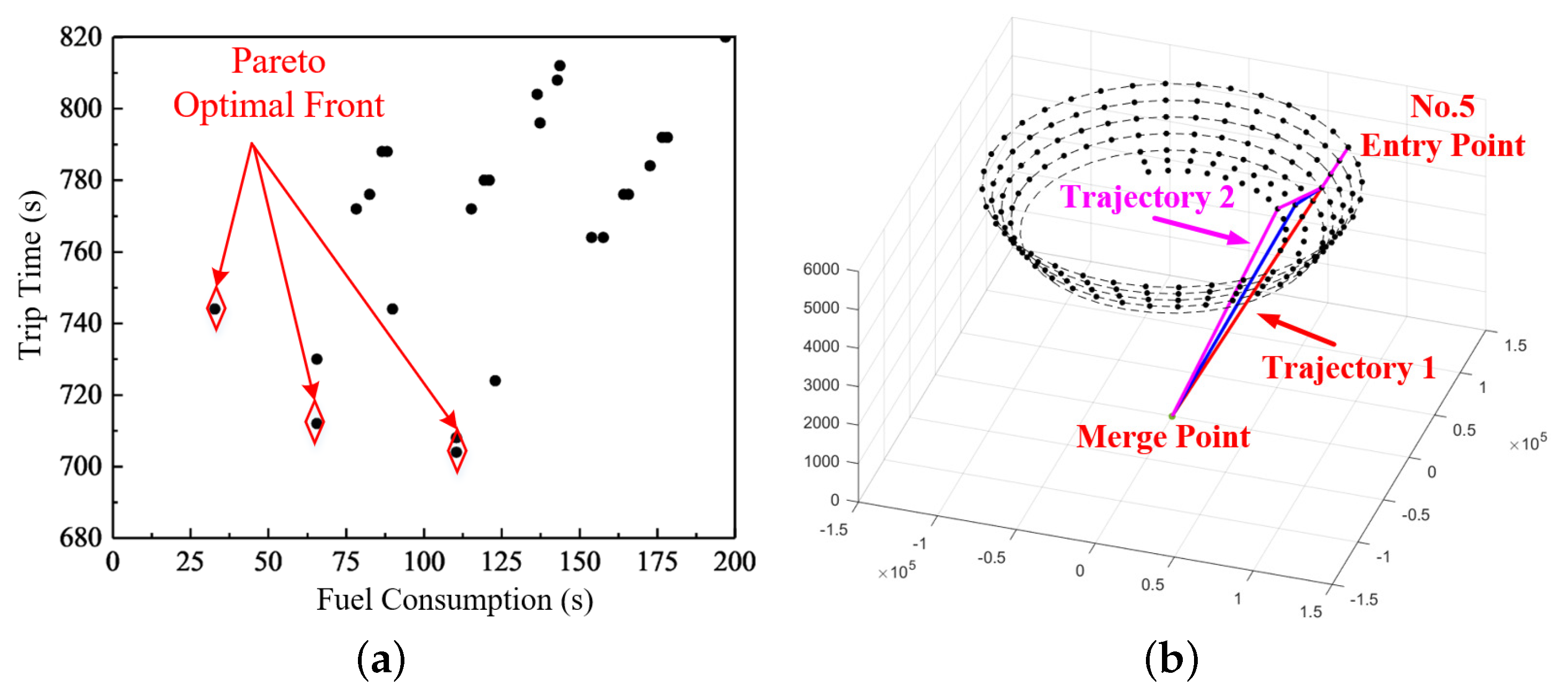
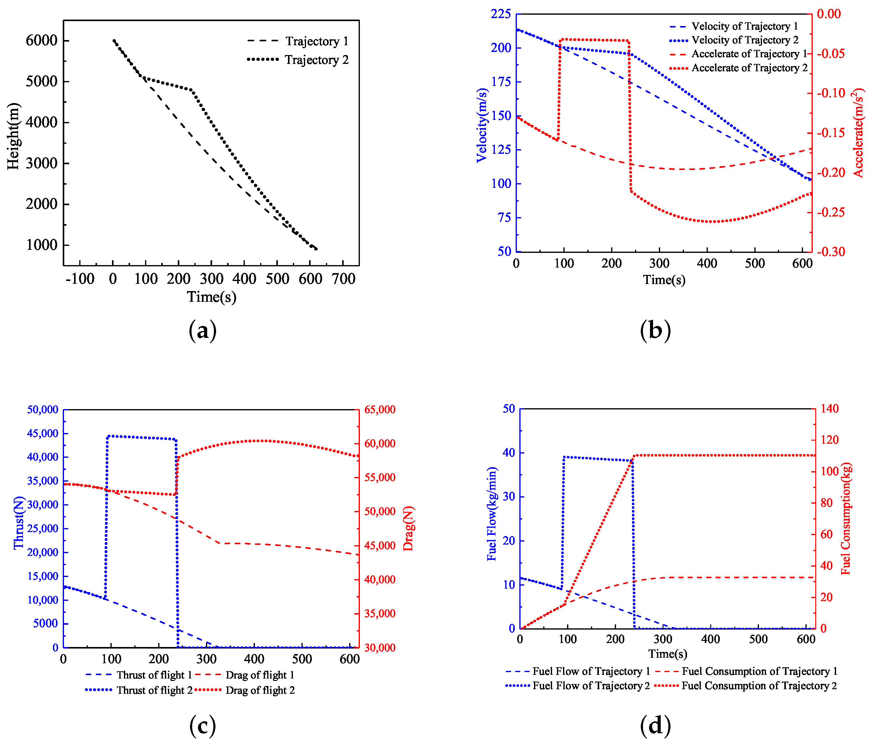
8.3. Single Aircraft Scenario

In the single aircraft scenario, the entry point is set to No.5. Some feasible solutions are shown in Figure 7a, where the Pareto-Optimal solutions are in the red diamond. The trajectories of such solutions are shown in Figure 7b. The convergence of Pareto front is shown in Figure 6.

For each Entry Point (EP), we search for the Optimal Trajectory with the least Fuel Consumption (OTFC) and the least Trip Time (OTTT) and get the Ideal Trajectory with Entropy-based TOPSIS method (ITET), respectively, as shown in

Table 3. The optimization results for each entry point.

EP	OTFC			OTTT			ITET
	FC	TT	Trajectory	FC	TT	Trajectory	FC	TT	Trajectory
1	32.8	744	1-1-1-1	110.4	704	1-1-1-27	32.8	744	1-1-1-1
2	32.8	744	2-2-2-2	110.4	704	2-2-2-28	32.8	744	2-2-2-2
3	32.8	744	3-3-3-3	110.4	704	3-3-3-29	32.8	744	3-3-3-3
4	32.8	744	4-4-4-4	110.4	704	4-4-4-30	32.8	744	4-4-4-4
5	32.8	744	5-5-5-5	110.4	704	5-5-5-31	32.8	744	5-5-5-5
6	32.8	744	6-6-6-6	110.4	704	6-6-6-32	32.8	744	6-6-6-6
7	32.8	744	7-7-7-7	110.4	704	7-7-7-33	32.8	744	7-7-7-7
8	32.8	744	8-8-8-8	110.4	704	8-8-8-34	32.8	744	8-8-8-8
9	32.8	744	9-9-9-9	110.4	704	9-9-9-35	32.8	744	9-9-9-9
10	32.8	744	10-10-10-10	110.4	704	10-10-10-36	32.8	744	10-10-10-10
11	32.8	744	11-11-11-11	110.4	704	11-11-11-37	32.8	744	11-11-11-11
12	32.8	744	12-12-12-12	110.4	704	12-12-12-38	32.8	744	12-12-12-12
13	32.8	744	13-13-13-13	110.4	704	13-13-13-39	32.8	744	13-13-13-13
14	78.3	800	14-14-14-13	122.9	720	14-14-14-39	78.3	800	14-14-14-13
15	128.3	856	15-15-14-13	153.9	760	15-15-15-39	136.44	812	15-15-15-26
16	182.1	924	16-16-14-13	196.9	816	16-16-16-39	196.9	816	16-16-16-39
17	237.6	992	16-15-14-13	247	872	17-17-16-39	247	872	17-17-16-39
18	292.8	1008	18-17-16-26	300.7	994	18-17-16-39	300.7	994	18-17-16-39
19	348.4	1076	18-17-16-26	356.1	1008	18-17-16-39	356.1	1008	18-17-16-39
20	414.5	1160	19-18-16-26	422.2	1092	19-18-16-39	422.2	1092	19-18-16-39
21	477.8	1240	20-19-16-26	485.5	1172	20-19-16-39	485.5	1172	20-19-16-39
22	545.6	1324	21-19-16-26	553.2	1256	21-19-16-39	553.2	1256	21-19-16-39
23	615.4	1412	22-19-16-26	623	1344	22-19-16-39	623	1344	22-19-16-39
24	688.8	1504	22-19-16-26	696.3	1436	22-19-16-39	696.3	1436	22-19-16-39
25	751.5	1588	26-28-31-14	759	1520	26-28-31-27	759	1520	26-28-31-27
26	682.9	1500	27-29-32-14	690.4	1432	27-29-32-27	690.4	1432	27-29-32-27
27	614.2	1412	28-30-33-14	621.8	1344	28-30-33-27	621.8	1344	28-30-33-27
28	545.6	1324	29-31-34-14	553.2	1256	29-31-34-27	553.2	1256	29-31-34-27
29	477.8	1240	30-31-34-14	485.5	1172	30-31-34-27	485.5	1172	30-31-34-27
30	414.5	1160	31-32-34-14	422.2	1092	31-32-34-27	422.2	1092	31-32-34-27
31	348.4	1076	32-33-34-14	356.1	1008	32-33-34-27	356.1	1008	32-33-34-27
32	292.8	1008	32-33-34-14	300.7	944	32-33-34-27	300.7	944	32-33-34-27
33	237.6	992	34-35-36-1	247	872	33-33-34-27	247	872	33-33-34-27
34	182.1	924	34-35-36-1	196.9	816	34-34-34-27	196.9	816	34-34-34-27
35	128.3	856	35-35-36-1	153.9	760	35-35-35-27	136.44	812	35-35-35-14
36	78.3	800	36-36-36-1	122.9	720	36-36-36-27	78.3	800	36-36-36-1

, where the “Trajectory” is named by the way-point number of each ring from the second-level to the fifth-level in the ICSAA. Please note that, for simplification, the number of level is omitted.

It is shown that fuel consumption gets higher with the trip time increasing. In view of that, we begin to gain insights into the reasons by investigating the dynamics parameters of aircraft during descent. As shown in Figure 7b, two different trajectories, Trajectory 1 (5-5-5-5) and Trajectory 2 (5-5-5-31), are generated. It is clear that the difference comes from the selection of the way-points at the fifth level, resulting in different flight path angles as mentioned in Section 2. Figure 8a shows the altitude evolves with time. It can be seen that the altitude of Trajectory 2 is always higher than that of Trajectory 1, and so is the velocity (Figure 8b), since we use the standard speed profile recommended by BADA, which shortens the trip time of Trajectory 2. In addition, for Trajectory 2, the time that the aircraft starts executing the CDO approach is around 250 s, as shown in Figure 8a, while the time for Trajectory 1 is about 150 s. Apparently, staying longer in the outside rings need more power according to the operation mode. When aircraft are executing continuous descent, the engine is idle or near-idle and the fuel burn is zero or near zero, as presented in Figure 8c,d. Therefore, more fuel burn of Trajectory 2 is observed.

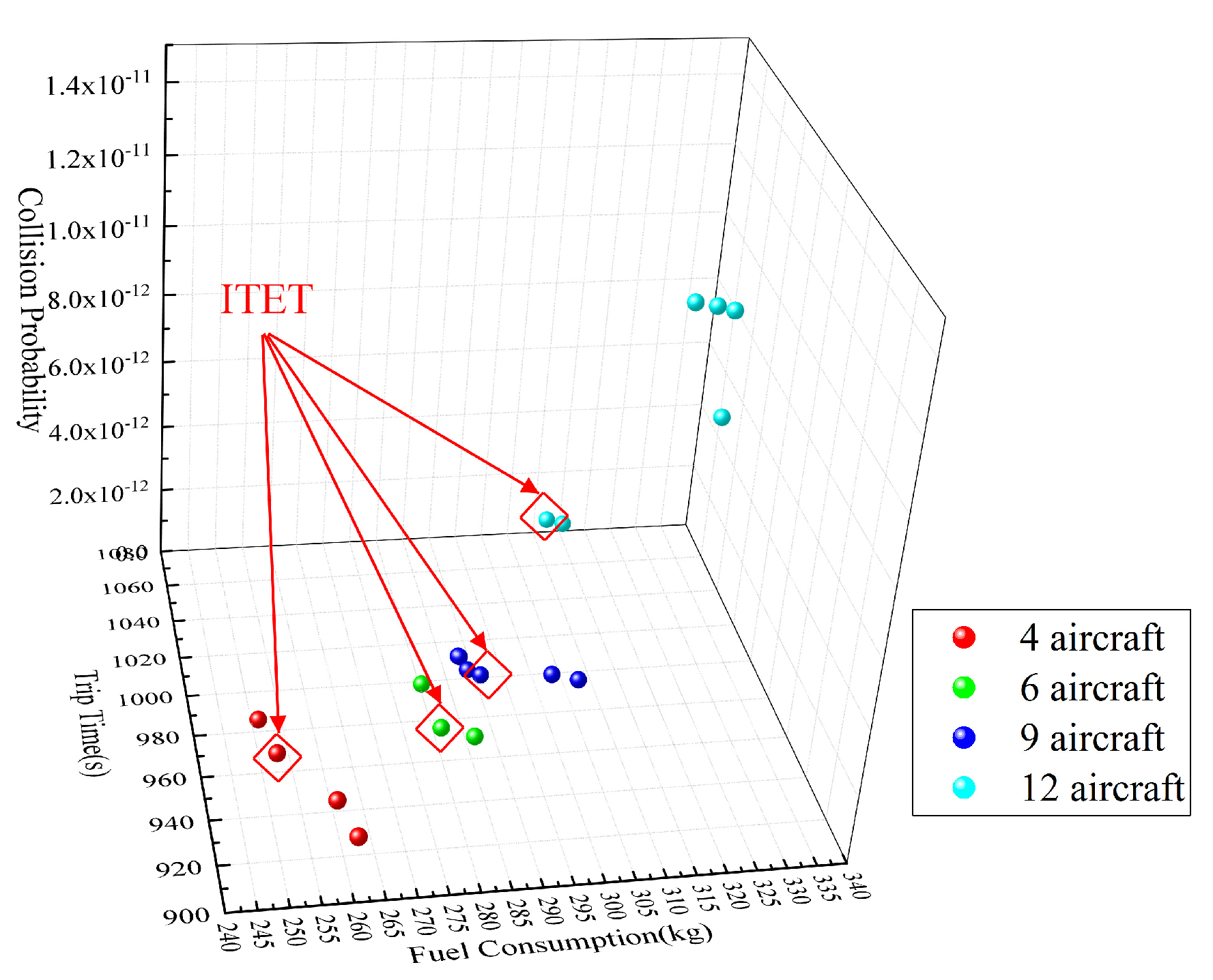
8.4. Multi-Aircraft Scenario

Safe and efficient operation in the high-density terminal area is always one of the great challenges in application of the CDO. In order to further investigate conflict-free trajectory planning based on ICSAA in the high-density situation, two traffic scenarios are designed: simultaneous arrival and continuous arrival, to explore the instantaneous and durative capacity performance of ICSAA.

8.4.1. Simultaneous Arrival

Four traffic scenarios with increasing density of 4, 6, 9, and 12 are designed to explore the transient operation performance in the ICSAA. For each scenario, the entry points are evenly spaced along the outermost ring. By estimating the time and speed of aircraft flying over the entry point in advance, optimal trajectories can be generated within 2 min. For each scenario, the Pareto optimal fronts are obtained with NSGA-II, and the collision probability of each solution is computed, as shown in Figure 9, where the solutiones of ITET, marked with red diamond, are obtained by OTE-MADM. In general, as the number of aircraft increases, average fuel consumption, average trip time and collision probability increase gradually. The results also suggest that, with the deepening of airspace congestion, the trade-off relationship is getting convergent.

Taking the scenario with 4 aircraft as an example, the trajectories corresponding to OTFC, OTTT, and ITET are shown in Figure 10. The main difference is still the choice of way-points at the fifth level of ICSAA, which also means the different flight path angles of trajectories. In the multi-aircraft scenario, choosing different flight path angle is helpful to resolve conflicts between aircraft, while having significant impact on the fuel consumption and trip time, as presented in

Table 4. The optimization results for the simultaneous arrival in the multi-aircraft scenario.

	4 Aircraft			6 Aircraft
	OTFC	OTTT	ITET	OTFC	OTTT	ITET
Total fuel consumption (kg)	1004.9	1052.5	1012.6	1682.6	1720.5	1689.3
Average fuel consumption (kg)	251.2	263.1	253.2	280.4	286.8	281.6
Reference total fuel consumption (kg)	974.9	974.9	974.9	1569.6	1569.6	1569.6
Reference average fuel consumption (kg)	243.7	243.7	243.7	261.6	261.6	261.6
Increase (kg)	7.5	19.4	9.4	18.8	25.2	20.0
Increase rate (%)	3.1	8.0	3.9	7.2	9.6	7.6
Total trip time (s)	3944.0	3712.0	3876.0	5992.0	5824.0	5856.0
Average trip time (s)	986.0	928.0	969.0	998.7	970.7	976.0
Reference total rip time (s)	3752.0	3752.0	3752.0	5768.0	5768.0	5768.0
Reference average trip time (s)	938.0	938.0	938.0	961.3	961.3	961.3
Increase (s)	48.0	−10.0	31.0	37.3	9.3	14.7
Increase rate (%)	5.1	−1.1	3.3	3.9	1.0	1.5
Collision rate	1.4 × 10−17	1.6 × 10−15	1.4 × 10−17	9.4 × 10−16	5.4 × 10−16	5.8 × 10−17
	9 Aircraft			12 Aircraft
	OTFC	OTTT	ITET	OTFC	OTTT	ITET
Total fuel consumption (kg)	2594.7	2755.9	2620.2	3680.2	3970.3	3680.2
Average fuel consumption (kg)	288.3	306.2	291.1	306.7	330.9	306.7
Reference total fuel consumption (kg)	2355.2	2355.2	2355.2	3135.4	3135.4	3135.4
Reference average fuel consumption (kg)	261.7	261.7	261.7	261.3	261.3	261.3
Increase (kg)	26.6	44.5	29.4	45.4	69.6	45.4
Increase rate (%)	10.2	17.0	11.3	17.4	26.6	17.4
Total trip time (s)	9108.0	8868.0	9012.0	12,512.0	12,140.0	12,512.0
Average trip time (s)	1012.0	985.3	1001.3	1042.7	1011.7	1042.7
Reference total rip time (s)	8584.0	8584.0	8584.0	11,400.0	11,400.0	11,400.0
Reference average trip time (s)	953.8	953.8	953.8	950.0	950.0	950.0
Increase (s)	58.2	31.6	47.6	92.7	61.7	92.7
Increase rate (%)	6.1	3.3	5.0	9.8	6.5	9.8
Collision rate	7.2 × 10−15	6.6 × 10−13	7.5 × 10−15	2.5 × 10−12	7.0 × 10−12	2.5 × 10−12

.

In order to further evaluate the optimization effect, we set ITET in the single aircraft scenario based on the Table 3 as reference. It means reference total fuel consumption is the sum of fuel consumption of each ITET and so is the reference total trip time. Then, we compare the reference value with the corresponding value of OTFC, OTTT, and ITET, as shown in Table 4, and the increase rate is shown in Figure 11. The results demonstrate that, as the number of aircraft increases, the average fuel consumption, average trip time and collision risk show an increasing trend. Under different congestion, when the ITET is picked, the increase rate of average fuel consumption is less than 20%, while the increase rate of average trip time is less than 10%. It is worth to note that there are some negative increases of fuel consumption of OTTT in some scenarios. The reason is that the ITET in the single aircraft scenario is selected as the reference, and, in some cases, the ITET in single aircraft scenario actually is the trajectory with the minimum trip time, so the fuel consumption is relatively large. But, in the multi-aircraft scenario, it is generally not possible to follow the trajectory with the maximal fuel consumption of the single aircraft scenario, since they have to take some maneuver to avoid conflicts. And such a maneuver does not take too much cost (i.e., fuel consumption and trip time) because the density of them is relatively low. Therefore, there is a path solution space with lower fuel consumption, and their fuel consumption could be less than the reference value.

In summary, when conducting CDO based on ICSAA in the simultaneous arrival, the optimization model we proposed could generate and get a set of optimized conflict-free four-dimensional trajectories for each aircraft. Based on a set of optimization results, we get a unique ideal solution by OTE-MADM, which makes accurate trade-offs among fuel consumption, trip time, and collision risk. In addition, compared the reference value, the increase of fuel consumption and trip time is optimized to an acceptable level.

8.4.2. Continuous Approach

In order to explore the continuous performance of CDO based on ICSAA, this paper has designed 4 traffic scenarios that four entry points are distributed uniformly in the outermost ring, and the number of aircraft increases from 4 to 16 by the step of 4, and the arrival time interval at the same entry point follows the Poisson distribution with the expectation of 2 min. In addition, the minimum separation at the entry points should be also guaranteed for safety.

We firstly generate planned trajectory for each aircraft based on ITET trajectory in Table 3. In order to further investigate the optimization ability of proposed models and algorithms, a Monte Carlo simulation was adopted to pick out the worst traffic pattern that contains the highest collision risk for each scenario. Flight trajectories in the ICSAA are then efficiently and optimally selected by proposed methods.

The Pareto optimal fronts and collision probability of each solution were obtained within 3 min, as presented in Figure 12, where the solution of ITET is marked with the red diamond. In general, with the increase of traffic density, the trade-off decision space between fuel consumption and trip time compresses. In the low-density scenario, the potential conflict between aircraft is less, so they have more choices, while, in the high-density scenario, the coupling degree among aircraft is high, and the airspace situation is complex, the solution space of conflict-free trajectories is reduced. For such optimization results, ITET is obtained with OTE-MADM, as presented in

Table 5. The optimization results for continuous arrival in the multi-aircraft scenario.

	4 Aircraft			8 Aircraft
	OTFC	OTTT	ITET	OTFC	OTTT	ITET
Total fuel consumption (kg)	1018.3	1127.2	1082.4	2075.9	2341.6	2111.2
Average fuel consumption (kg)	254.6	281.8	270.6	259.5	292.7	263.9
Reference total fuel consumption (kg)	974.9	974.9	974.9	1949.8	1949.8	1949.8
Reference average fuel consumption (kg)	243.7	243.7	243.7	243.7	243.7	243.7
Increase (kg)	10.9	38.1	26.9	15.8	49	20.2
Increase rate (%)	4.47	15.63	11.04	6.48	20.11	8.29
Total trip time (s)	4020	3824	3840	7972	7744	7872
Average trip time (s)	1005	956	960	996.5	968	984
Reference total rip time (s)	3752	3752	3752	7504	7504	7504
Reference average trip time (s)	938	938	938	938	938	938
Increase (s)	67	18	22	58.5	30	46
Increase rate (%)	7.14	1.92	2.35	6.24	3.20	4.90
Collision rate	2.9 × 10−14	1.2 × 10−18	1.8 × 10−18	6.3 × 10−13	1.2 × 10−15	7.2 × 10−15
	12 Aircraft			16 Aircraft
	OTFC	OTTT	ITET	OTFC	OTTT	ITET
Total fuel consumption (kg)	3415.5	3662.7	3585.1	5033.4	5143.8	5066.1
Average fuel consumption (kg)	284.6	305.2	298.8	314.6	321.5	316.6
Reference total fuel consumption (kg)	2924.7	2924.7	2924.7	3899.6	3899.6	3899.6
Reference average fuel consumption (kg)	243.7	243.7	243.7	243.7	243.7	243.7
Increase (kg)	40.9	61.5	55.1	70.9	77.8	72.9
Increase rate (%)	16.78	25.24	22.61	29.09	31.92	29.91
Total trip time (s)	12,248	11,832	11,872	16,840	16,776	16,816
Average trip time (s)	1020.7	986	989.3	1052.5	1048.5	1051
Reference total rip time (s)	11,256	11,256	11,256	15,008	15,008	15,008
Reference average trip time (s)	938	938	938	938	938	938
Increase (s)	82.7	48	51.3	114.5	110.5	113
Increase rate (%)	8.82	5.12	5.47	12.21	11.78	12.05
Collision rate	3.4 × 10−12	1.9 × 10−15	1.8 × 10−14	2.5 × 10−12	7.0 × 10−12	2.5 × 10−12

. The results demonstrate that the average fuel consumption and the average trip time present an increasing trend with the number of aircraft rises. Similar to the previous subsection, compared with the reference value (i.e., reference total fuel consumption, reference total trip time, etc.), as shown in the Figure 13, all the increase rate of the fuel consumption and the trip time is less than 30% and 15%, respectively, with the number of aircraft increasing.

In conclusion, in the continuous approach scenario, the proposed algorithm is still efficient and reliable. Although the additional ratio of average fuel consumption and trip time after optimization continue to increase with the increase of traffic density, it is still at an acceptable level. OTE-MADM could also make a good trade-off among fuel consumption, trip time, and collision probability. It can effectively support the high-performance operation requirements of high-density terminal area and help to promote the level of coordination between ATC and airlines under TBO mode.

9. Conclusions and Future Work

Improving flexibility of approach airspace is one of cornerstone for implementing CDO especially in high-density traffic scenarios. Inspired by traditional PMS, this paper broke through the traditional rigid terminal airspace structure by designing ICSAA and its operational procedures to deliver Omni-directional CDO. A multi-objective trajectory optimization model aiming at minimizing fuel consumption and trip time was solved by NSGA-II. In order to provide decision-making support to air traffic controller, the best trade-off was determined using entropy-based TOPSIS from the perspective of safety, efficiency and economy.

The proposed models and algorithms were validated in the single aircraft scenario, the multi-aircraft scenarios with simultaneous and continuous arrivals to gain insights into the interplay of traffic demand and given objectives. The results verified the effectiveness and efficiency of optimal CDO operation in ICSAA dealing with complex traffic patterns, which demonstrates the potential of CDO operation in high-density terminal area and enables the application of TBO.

This paper is a preliminary exploration of CDO trajectory planning in the novel airspace. Further research shall be carried out to solve the limitations and to facilitate the transition from theoretical studies to real-world practice.

• The ICSAA was designed based on an artificial airspace irrespective to terrain, obstacles, noise abatement, airspace restriction and runway configurations, etc. The very essential work is to adapt the ICSAA to a real airport and thoroughly validate the effectiveness by both fast-time simulations and Human-In-The-Loop (HITL) experiments.
• Aircraft positioning error was considered in trajectory selection in this paper. However, more realistic uncertain factors, like flight control error, meteorological conditions, stochastic runway scheduling, etc., shall also be included in robust CDO trajectory planning and implementation.
• Human-machine system is another emerging topic in future autonomous ATM. The decision-making by machine shall be transparent and understandable, which allows air traffic controllers and pilots to take over automated equipment at any time safely. It means the cognition of human and machine needs to be strongly synchronized [42]. For automated CDO trajectory planning and negotiation in flexible airspace, designing transparent Decision Support System (DSS) based on explainable Artificial Intelligence(AI) would be an indispensable approach to enhance human cognition, operational efficiency, and safety, especially for a high-density traffic scenario.

References

1. Sáez, R.; Prats, X.; Polishchuk, T.; Polishchuk, V.; Schmidt, C. Automation for Separation with Continuous Descent Operations: Dynamic Aircraft Arrival Routes. J. Air Transp. 2020, 28, 1–11. [Google Scholar] [CrossRef]
2. Sun, M.; Rand, K.; Fleming, C. 4 Dimensional waypoint generation for conflict-free trajectory based operation. Aerosp. Sci. Technol. 2019, 88, 350–361. [Google Scholar] [CrossRef]
3. Clarke, J.P.B.; Ho, N.T.; Ren, L.; Brown, J.A.; Elmer, K.R.; Tong, K.O.; Wat, J.K. Continuous descent approach: Design and flight test for Louisville Inter-national Airport. J. Aircr. 2004, 41, 1054–1066. [Google Scholar] [CrossRef]
4. SheHRESTA, S.; Neskovic, D.; Williams, S.S. Analysis of continuous descent benefits and impacts during daytime operations. In Proceedings of the 8th USA/Europe Air Traffic Management Research and Development Seminar (ATM2009), Napa, CA, USA, 29 June–2 July 2009. [Google Scholar]
5. ICAO. Continuous Descent Operations (CDO) Manual; International Civil Aviation Organization: Montréal, QC, Canada, 2010. [Google Scholar]
6. Jin, L.; Cao, Y.; Sun, D. Investigation of potential fuel savings due to continuous-descent approach. J. Aircr. 2013, 50, 807–816. [Google Scholar] [CrossRef] [Green Version]
7. Turgut, E.T.; Usanmaz, O.; Cavcar, M.; Dogeroglu, T.; Armutlu, K. Effects of Descent Flight-Path Angle on Fuel Consumption of Commercial Aircraft. J. Aircr. 2018, 56, 313–323. [Google Scholar] [CrossRef]
8. Fricke, H.; Seiß, C.; Herrmann, R. Fuel and energy benchmark analysis of continuous descent operations. Air Traffic Control. Q. 2015, 23, 83–108. [Google Scholar] [CrossRef]
9. Andreeva-Mori, A.; Suzuki, S.; Itoh, E. Scheduling of arrival aircraft based on minimum fuel burn descents. ASEAN Eng. J. 2011, 1, 25–38. [Google Scholar]
10. Enea, G.; Bronsvoort, J.; Mcdonald, G. Trade-Off between Optimal Profile Descents, Runway Throughput and Net Fuel Benefit, Preliminary Discussion and Results. In Proceedings of the 17th AIAA Aviation Technology, Integration, and Operations Conference, Denver, CO, USA, 5–9 June 2017; p. 4486. [Google Scholar]
11. Park, S.G.; Clarke, J.P. Optimal control based vertical trajectory determination for continuous descent arrival procedures. J. Aircr. 2015, 52, 1469–1480. [Google Scholar] [CrossRef]
12. Jia, Y.; Cai, K. The Trade-off Between Trajectory Predictability and Potential Fuel Savings for Continuous Descent Operations. In Proceedings of the 2018 IEEE/AIAA 37th Digital Avionics Systems Conference (DASC), London, UK, 23–27 September 2018; pp. 1–6. [Google Scholar]
13. Murrieta-Mendoza, A.; Ruiz, H.; Botez, R.M.; Supérieure, T. Vertical reference flight trajectory optimization with the particle swarm optimisation. In Proceedings of the 36th IASTED International Conference on Modelling, Identification and Control (MIC 2017), Innsbrunck, Austria, 20–21 February 2017. [Google Scholar]
14. Samà, M.; D’Ariano, A.; Palagachev, K.; Gerdts, M. Integration methods for aircraft scheduling and trajectory optimization at a busy terminal manoeuvring area. OR Spectr. 2019, 41, 641–681. [Google Scholar] [CrossRef]
15. Tian, Y.; He, X.; Xu, Y.; Wan, L.; Ye, B. 4D Trajectory Optimization of Commercial Flight for Green Civil Aviation. IEEE Access 2020, 8, 62815–62829. [Google Scholar] [CrossRef]
16. Zhang, M.; Filippone, A.; Bojdo, N. Using Trajectory Optimization to Minimize Aircraft Noise Impact. INTER-NOISE and NOISE-CON Congress and Conference Proceedings. Inst. Noise Control Eng. 2017, 255, 4003–4013. [Google Scholar]
17. Rosenow, J.; Förster, S.; Lindner, M.; Fricke, H. Multicriteria-Optimized Trajectories Impacting Today’s Air Traffic Density, Efficiency, and Environmental Compatibility. J. Air Transp. 2019, 27, 8–15. [Google Scholar] [CrossRef]
18. Dalmau, R.; Prats, X.; Baxley, B. Fast sensitivity-based optimal trajectory updates for descent operations subject to time constraints. In Proceedings of the 2018 IEEE/AIAA 37th Digital Avionics Systems Conference (DASC), London, UK, 23–27 September 2018; pp. 1–10. [Google Scholar]
19. Seenivasan, D.B.; Olivares, A.; Staffetti, E. Multi-aircraft optimal 4D online trajectory planning in the presence of a multi-cell storm in development. Transp. Res. Part C Emerg. Technol. 2020, 110, 123–142. [Google Scholar] [CrossRef]
20. Kendall, A.P.; Clarke, J.P. Stochastic Optimization of Area Navigation Noise Abatement Arrival and Approach Procedures. J. Guid. Control Dyn. 2020, 43, 863–869. [Google Scholar] [CrossRef]
21. Alam, S.; Nguyen, M.H.; Abbass, H.A.; Lokan, C. Multi-aircraft dynamic continuous descent approach methodology for low-noise and emission guidance. J. Aircr. 2011, 48, 1225–1237. [Google Scholar] [CrossRef]
22. Favennec, B.; Symmans, T.; Houlihan, D.; Vergne, K.; Zeghal, K. Point Merge Integration of Arrival Flows Enabling Extensive RNAV Application and Continuous Descent–Operational Services and Environment Definition. 2010. Available online: https://www.eurocontrol.int/sites/default/files/2019-06/point-merge-osed-v2.0-2010_1.pdf (accessed on 26 January 2021).
23. Errico, A.; Di Vito, V. Aircraft operating technique for efficient sequencing arrival enabling environmental benefits through CDO in TMA. In Proceedings of the AIAA Scitech 2019 Forum, San Diego, CA, USA, 7–11 January 2019; p. 1363. [Google Scholar]
24. Hong, Y.; Choi, B.; Lee, K.; Kim, Y. Dynamic robust sequencing and scheduling under uncertainty for the point merge system in terminal airspace. IEEE Trans. Intell. Transp. Syst. 2017, 19, 2933–2943. [Google Scholar] [CrossRef]
25. Glover, W.; Lygeros, J. A multi-aircraft model for conflict detection and resolution algorithm evaluation. HYBRIDGE Deliv. D 2004, 1, 3. [Google Scholar]
26. Center, E.E. User Manual for the Base of Aircraft Data (BADA); Revision 3.11; EEC Note: Belgium, 2013; Available online: https://www.eurocontrol.int/publication/user-manual-base-aircraft-data-bada (accessed on 26 January 2021).
27. Seenivasan, D.B.; Olivares, A.; Staffetti, E. Optimal 4D Trajectory Planning for Multiple Aircraft in Continuous Descent Operations. In Proceedings of the 8th European Conference for Aeronautics and Aerospace Science (EUCASS), Madrid, Spain, 1–4 July 2019; Available online: https://www.eucass.eu/doi/EUCASS2019-0544.pdf (accessed on 26 January 2021).
28. Filippone, A. Aircraft noise prediction. Prog. Aerosp. Sci. 2014, 68, 27–63. [Google Scholar] [CrossRef]
29. Deb, K.; Pratap, A.; Agarwal, S.; Meyarivan, T.A.M.T. A fast and elitist multi-objective genetic algorithm: NSGA-II. IEEE Trans. Evol. Comput. 2002, 6, 182–197. [Google Scholar] [CrossRef] [Green Version]
30. Yu, X.; Lu, Y.Q.; Yu, X. Evaluating Multi-objective Evolutionary Algorithms Using MCDM Methods. IEEE Math. Probl. Eng. 2018, 2018, 1–14. [Google Scholar]
31. Wątróbski, J.; Jankowski, J.; Ziemba, P.; Karczmarczyk, A.; Zioło, M. Generalised framework for multi-criteria method selection. Omega 2019, 86, 107–124. [Google Scholar] [CrossRef]
32. Dos Santos, B.M.; Godoy, L.P.; Campos, L.M.S. Performance evaluation of green suppliers using entropy-TOPSIS-F. J. Clean. Prod. 2019, 207, 498–509. [Google Scholar] [CrossRef]
33. Wu, Z.; Li, J.; Zuo, J.; Li, S. Path planning of UAVs based on collision probability and Kalman filter. IEEE Access 2018, 6, 34237–34245. [Google Scholar] [CrossRef]
34. Zou, Z.; Yun, Y.; Sun, J. Entropy method for determination of weight of evaluating indicators in fuzzy synthetic evaluation for water quality assessment. J. Environ. Sci. 2006, 18, 1020–1023. [Google Scholar] [CrossRef]
35. Taheriyoun, M.; Karamouz, M.; Baghv, A. Development of an entropy-based fuzzy eutrophication index for reservoir water quality evaluation. Iran. J. Environ. Health Sci. Eng. 2010, 7, 1–14. [Google Scholar]
36. Kumar, R.; Singh, S.; Bilga, P.S.; Jatin, K.; Singh, J.; Singh, S.; Scutaru, S.-M.; Pruncu, C.I. Revealing the Benefits of Entropy Weights Method for Multi-Objective Optimization in Machining Operations: A Critical Review. J. Mater. Res. Technol. 2021, 10, 1471–1492. [Google Scholar] [CrossRef]
37. Zhu, Y.; Tian, D.; Yan, F. Effectiveness of Entropy Weight Method in Decision-Making. Math. Probl. Eng. 2020, 2020, 1–5. [Google Scholar] [CrossRef]
38. Sałabun, W. The mean error estimation of TOPSIS method using a fuzzy reference models. J. Theor. Appl. Comput. Sci. 2013, 7, 40–50. [Google Scholar]
39. Sałabun, W.; Wątróbski, J.; Shekhovtsov, J. Are MCDA Methods Benchmarkable? A Comparative Study of TOPSIS, VIKOR, COPRAS, and PROMETHEE II Methods. Symmetry 2020, 12, 1549. [Google Scholar] [CrossRef]
40. Chen, P. Effects of normalization on the entropy-based TOPSIS method. Expert Syst. Appl. 2019, 136, 33–41. [Google Scholar] [CrossRef]
41. Hwang, C.L.; Yoon, K.P. Multiple Attribute Decision Making: Methods and Applications; Springer: New York, NY, USA, 1981. [Google Scholar]
42. Sáez Nieto, F.J. The long journey toward a higher level of automation in ATM as safety critical, sociotechnical and multi-Agent system. Proc. Inst. Mech. Eng. Part G J. Aerosp. Eng. 2016, 230, 1533–1547. [Google Scholar] [CrossRef]
Figure 1. The route structure of Point Merge.
Sustainability 13 01354 g001
Figure 2. The 3-dimensional graph (a) and the top view (b) of the Inverted Crown-Shaped Arrival Airspace (ICSAA).
Sustainability 13 01354 g002
Figure 3. The fitting curve of the speed profile.
Sustainability 13 01354 g003
Figure 4. Non-dominated Sorting Genetic Algorithm with Elitist Strategy (NSGA-II) procedure.
Sustainability 13 01354 g004
Figure 5. The collision area of aircraft.
Sustainability 13 01354 g005
Figure 6. The comparison of convergence of different algorithms.
Sustainability 13 01354 g006
Figure 7. Trajectory optimization in the single aircraft scenario: (a) Pareto fronts. (b) Optimized trajectories.
Sustainability 13 01354 g007
Figure 8. The performance parameter of aircraft implementing Continuous Descent Operations (CDO): (a) The height change; (b) the velocity and acceleration rate change; (c) the thrust and drag change; (d) the fuel consumption and fuel flow rate change.
Sustainability 13 01354 g008
Figure 9. Pareto optimal fronts for simultaneous arrival in the multi-aircraft scenario.
Sustainability 13 01354 g009
Figure 10. Comparison of the optimized trajectories.
Sustainability 13 01354 g010
Figure 11. Increased proportion of fuel consumption and trip time comparing with the ideal ones (for the simultaneous arrivals).
Sustainability 13 01354 g011
Figure 12. Pareto optimal fronts for continuous arrival in the multi-aircraft scenario.
Sustainability 13 01354 g012
Figure 13. Increased proportion of fuel consumption and trip time for continuous arrival in the multi-aircraft scenario.
Sustainability 13 01354 g013