Article

Sustainability Assessment of Public Transport, Part II—Applying a Multi-Criteria Assessment Method to Compare Different Bus Technologies

Environmental Technology and Management and Biogas Research Center (BRC), Department of Management and Engineering, Linköping University, SE-581 83 Linköping, Sweden
*
Author to whom correspondence should be addressed.
Sustainability 2021, 13(3), 1273; https://doi.org/10.3390/su13031273
Submission received: 17 December 2020 / Revised: 11 January 2021 / Accepted: 22 January 2021 / Published: 26 January 2021
(This article belongs to the Special Issue Multi-criteria Decision Making and Sustainable Transport)

Abstract

:
Many Swedish regional transport authorities want bus fleets driven on renewable fuels. However, it may be difficult to know what technology, or combination of technologies, to choose. There is a need for improved knowledge and supportive methods for sustainability assessments that can support public procurement processes. In the companion article (Part I), a multi-criteria assessment (MCA) method for assessments of public bus technologies’ sustainability was established, consisting of four key areas and 12 indicators. In this article, the purpose is to apply the method established in part I on different bus technologies by looking at a general Swedish case and assessing buses driven on diesel, Hydrotreated Vegetable Oil (HVO), Fatty Acid Methyl Ester (FAME), ethanol, natural gas, biomethane and electricity. Each technology is assessed on a scale from Very Poor to Very Good according to the indicators: technical maturity, daily operational availability, total cost of ownership, need for investments in infrastructure, cost stability, non-renewable primary energy efficiency, greenhouse gas emission savings, air pollution, noise, local/regional impact on land and aquatic environments, energy security and sociotechnical systems services. The results show the strengths and weaknesses of each technology, which are later discussed. We also critically reflect upon the usefulness and accuracy of the MCA method.

1. Introduction

Transport systems have a wide range of negative sustainability effects [1], for example, contributing to global warming [2]; pollution of air, water and land causing health problems and other impacts [3,4]; noise [5,6]; and loss of biodiversity (e.g., [7,8,9]). To deal with such challenges, organizations of different kinds take measures to transform the transport system in a sustainable direction. One such type of organization, which is focused on in this article, is public transport authorities. Public transport authorities are responsible for the procurement of regional public transports such as bus transports, which is often an important public transport mode.
When studying public transport authorities, Sweden is an interesting case to explore. In line with national and EU objectives, most regional public transport authorities in Sweden have transformed the bus fleet in a renewable direction. Using green public procurement (GPP), they have managed to significantly lower the share of fossil fuels [10]. However, there are several renewable bus technologies available to choose between, such as biomethane, ethanol, FAME (Fatty Acid Methyl Ester), HVO (Hydrotreated Vegetable Oil) and electric vehicles, and the regions and other actors struggle with how to know which alternative, or combination of alternatives, is best suited for them.
This article is the second of two associated articles. According to the literature review presented in the first article (Part I, Ammenberg and Dahlgren, 2020 (“Part I” is used to refer to this first article in the remaining parts of the article)), there are important barriers to overcome to further strengthen the uptake and application of green or sustainable public procurement (GoSPP) practices (e.g., [11,12,13]). Important challenges include the lack of knowledge and trustworthy information, and there is a need for simple but broad assessment tools [14] with relevant procurement criteria that help the GoSPP process (e.g., [15]).
Part I motivates that multi-criteria assessment (MCA) methods can be used as appropriate tools for supporting GoSPP and lists criteria for effectiveness and efficiency of such methods. Further on, it establishes an MCA method for sustainability assessment of different bus technologies.

Aim and Scope

The purpose of this article, Part II, is to apply the multi-criteria assessment (MCA) method, developed in Part I, on different bus technologies to do the following:
  • Test the method and critically reflect upon its application and usefulness,
  • Compare the different bus technologies, including buses driven on biomethane, ethanol, FAME, HVO and electricity, and diesel and natural gas as reference technologies.
This article thus deals with the general methodological problem of how to conduct sustainability assessments of transport technologies and intends to contribute to improved knowledge of the sustainability performance of different bus technologies.

2. Methods

The methodology used to develop the MCA method is thoroughly presented and motivated in Part I. This MCA method includes four key areas covered by twelve indicators (Table 1). Each indicator has a scale, from Very Poor to Very Good, which is used to assess the different bus technologies. In this chapter, the bus technologies that are assessed are specified and the assessment process is presented, including data collection and uncertainty assessment.

2.1. Assessed Bus Technologies

Seven bus technologies have been assessed, as they are all reasonable options for regional public bus transport in Sweden, namely, biomethane, diesel, electricity, ethanol, FAME, HVO and natural gas. All buses are assumed to be new 12-m Euro VI buses. However, a difference from reality is that all fuels are assumed to be used unblended, that is, no blending of, for example, diesel and RME. In reality (at least in a Swedish context), biomethane (there is a high biomethane content in the Swedish vehicle gas on average—the share is over 90%) can be mixed with natural gas and diesel is sold with different shares of FAME and HVO and so forth, and there are electric hybrid buses that can mix the use of electricity with, for example, HVO or biomethane.
For each technology, some assumptions have been made in relation to the indicators to mirror Swedish conditions, for example, regarding electricity production and substrates for biogas production (Table 2). In several cases, however, alternative assumptions and how they would affect the results are mentioned and discussed. Worth noting is that we have assumed HVO to have a content of Palm Fatty Acid Distillate (PFAD), but due to new regulations, this may change. For electric buses, the “extreme” cases of large batteries and night charging as well as small batteries and fast charging have been used to show the large span. When only one result is showed, it has been estimated that the results are quite similar no matter the battery size or recharging infrastructure.

2.2. Assessment Process

In the assessment process, each indicator was assessed for the respective bus technology, largely based on literature studies. This mainly included information from journal articles, theses, technical reports and governmental statistics. Inputs from the participating stakeholders (Appendix A) were also contributed, chosen to complement the knowledge of the authors and other participants. The assessment was done from the current Swedish context.
As described in Part I, the method development process started with two student projects that contributed to early versions of the MCA method, and the students also carried out assessments that were discussed with stakeholders. The method was then further developed (in several steps) and additional data collected, considering the input from the participants. This improved version of the method and the results were sent out on a review round to a number of relevant actors who got the chance to comment. These actors are experts in their areas, chosen to complement the knowledge of the authors and other participants. Considering this input, the authors updated the method and results again.
In addition to the assessment of the scales, that is, from Very Poor (red) to Very Good (dark green), the certainty was also assessed for each indicator and technology. The focus here was on to what extent we found enough relevant and trustworthy information. For this assessment, we used a three-step scale:
  • ***; low uncertainty;
  • **; some uncertainty;
  • *; high uncertainty.

3. Results

In this section, the results from the assessment are presented for each key area and indicator. The indicators are briefly introduced—further information on their relevance, formulation and scales for assessment can be found in Part I. Commonly, each section starts with diesel, as it is a kind of reference technology that dominated the public bus transportation earlier. Next follows the technologies most similar to diesel (i.e., HVO, FAME and ethanol), and finally, natural gas, biomethane and electricity are addressed.

3.1. Technical Performance

Two indicators deal with the technical performance: technical maturity and daily operational availability.

3.1.1. Technical Maturity

The indicator of technical maturity assesses the stage of development and implementation of the bus technologies. The scale goes from possibly coming technologies (Very Poor) to well-established technologies on both the national and international market (Very Good).
Diesel was long the standard option for buses in Sweden [18,19,20], and in many parts of the world, it still is [21]. Therefore, diesel received the score Very Good (Table 3). Diesel buses are also used for HVO and FAME, the latter with some slight modifications of the bus engine. Therefore, these two alternatives are also assessed as Very Good. Buses using ethanol and methane gas (i.e., compatible with biomethane and natural gas) have both been used for several decades in Sweden [18,19], and there are experiences of these buses in several different regions across the country. Buses using vehicle gas are still popular, while the number of ethanol buses has decreased in recent years. Several other countries also have gas buses [22], while the number of ethanol buses is generally smaller [21,22]. Because of their more widespread use, biomethane and natural gas were considered Very Good. To use ethanol for bus transportation is a well-proven technology, but the lower degree of use means less-developed support networks, and, therefore, this technology was judged as Good. Electric buses are relatively new, but the technology is commercially implemented and proven to work well in several cases. The number of buses is relatively low in Sweden—less than 1% of all buses [19]—and the situation is similar in the majority of the world [23]. This resulted in Satisfactory. However, the number of electric buses is increasing worldwide, especially in China [21,24]. Thus, the technical readiness level could improve fast.
The technical functionality also depends on the availability of fuels or electricity of desirable quality. It should be noted that HVO has only been used in Sweden since 2015 [25]. Back then, HVO represented 1% of the fuel used for public buses, then rapidly increasing to over 40% in 2017 [18]. In many countries, natural gas is the norm, while the use of biomethane for transportation is less common or non-existing (cf. [26]). Limitations on the capacity of the electricity production and distribution (systems) can, in some regions, influence the possibilities to expand large-scale electric transportation projects [27]. Such considerations can be critical in connection with a real case assessment, and such context-specific fuel aspects should then complement the relatively generic results in Table 3.

3.1.2. Daily Operational Availability

The indicator of daily operational availability gauges if, and to what extent, refueling or recharging negatively influence the preferred timetable and if additional vehicles are needed due to this. A three-step scale was used, where Very Poor means that refueling and recharging have a significant negative impact on the desired timetables or require additional buses, while Very Good means that there are no such negative effects related to refueling or recharging. A medium-sized European city usually requires a bus driving range of around 300 km/day to be able to carry out the daily duties without refueling/recharging [28], which is well in line with information on Linköping city [29], the largest city among the participating regions (Linköping city has about 160,000 inhabitants and is situated in the region of Östergötland). Thus, 300 km/day is used as a reference range.
Diesel buses have a range of somewhere between 450 and 900 km [28,30,31,32,33] (throughout the article, intervals presented like this indicate that the referenced sources had values somewhere in between those values. All sources did not have the same value; instead, the interval is a range of likely values), leading to the score Very Good (Table 4). HVO, FAME and ethanol can all be used in diesel buses with similar tanks, while their lower energy contents can lead to shorter ranges [28], especially for ethanol, which has the lowest energy content and an estimated range of 400–600 km [28]. Nevertheless, all three qualify as Very Good. Natural gas and biomethane give shorter ranges than the liquid fuels, and commonly used tank volumes provide ranges of 250–400 km [28,30,31]. For these gaseous fuels, there are two different refueling options—either refueling slowly at night or refueling quickly, similar to the liquid fuels [34]. It is thus possible for natural gas and biomethane to be either Satisfactory or Very Good. For electricity, there are also two main options: to use buses with small batteries that need fast charging for a few minutes at selected stops on the route, or to use large batteries and slow depot charging during the night. Fast charging requires time during routes, which may negatively influence timetables or require additional buses. This reduces the flexibility—for example, it may not be possible to gain lost time by skipping the planned pause (extra time) at the end-stop if recharging is required. However, with a well-adapted infrastructure and depending on the desirable timetables, the negative impact may become acceptable. Slow charging with a large battery can provide ranges of around 300 km [35,36]. Consequently, depending on what technique is chosen and the regional conditions and expectations, the score for electric buses ranges between Very Poor and Very Good.
It should be noted that the results regarding daily operational availability are very dependent on what daily range is needed and used for the assessment. If longer ranges are required (cf. [37]), the liquid fuels will turn out as most favorable. From our communication with the bus providers, there seems to be some flexibility regarding their bus models’ design and capacity when a large number of buses are bought. For example, it may be possible to adapt the tank and battery sizes to fit local requirements.

3.2. Economic Performance

For comparison of economic performance, three indicators were included: total cost of ownership, need for investments in infrastructure and cost stability.

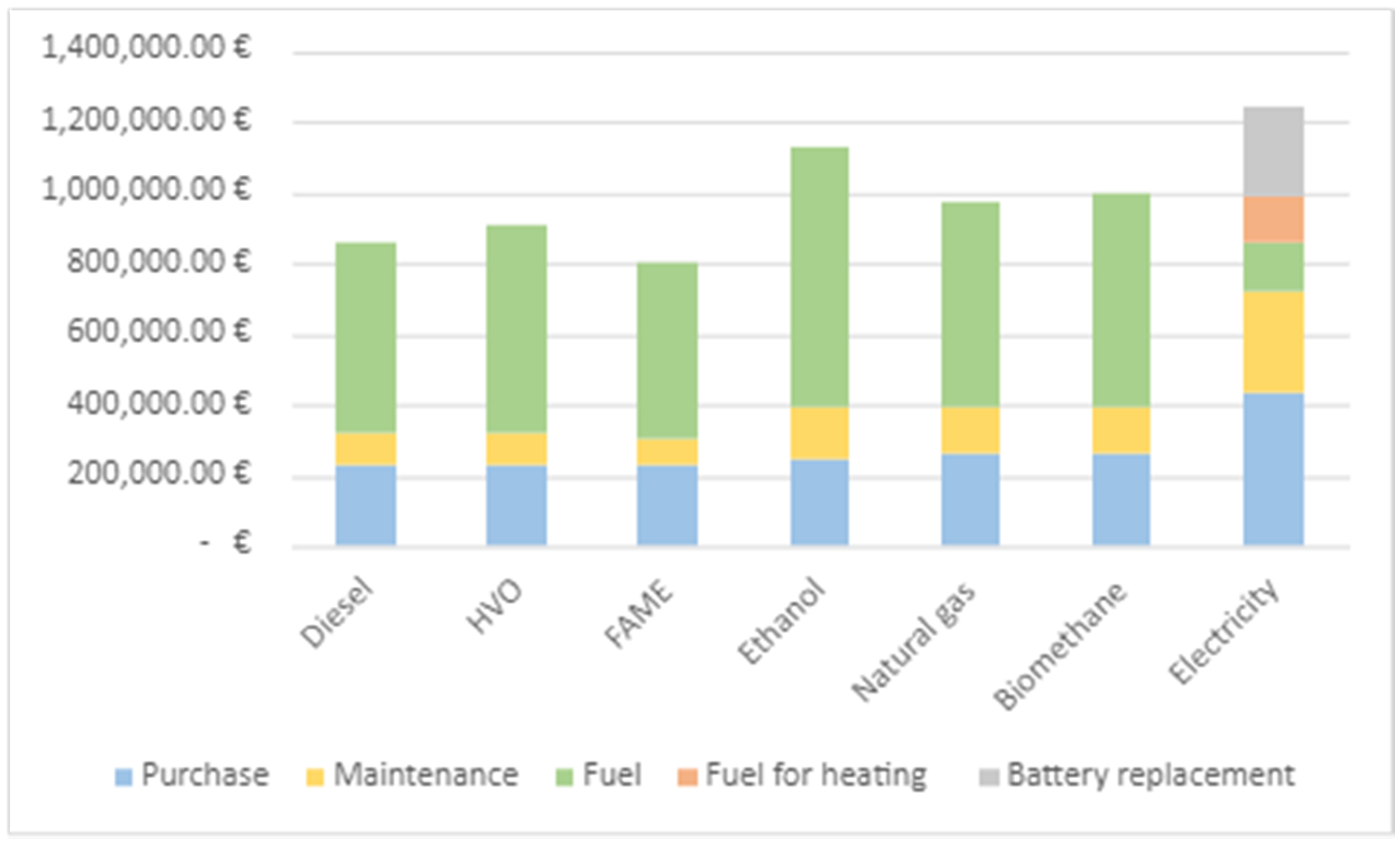
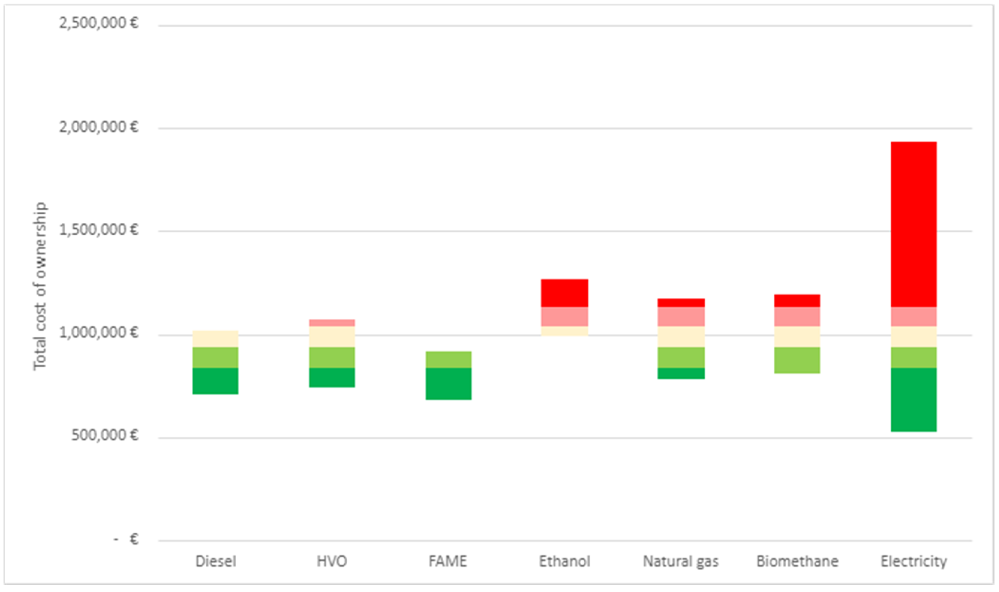
3.2.1. Total Cost of Ownership

Total cost of ownership comprises costs related to vehicle purchase, fuel consumption and maintenance/repair over the 10-year period and accounts for the residual value. The scale is based on a comparison of the studied alternatives, with the least expensive option set to Very Good.
Diesel buses, starting with purchasing, cost around 220,000–260,000 euro, and the range is similar for HVO and FAME [28,32,38,39,40,41,42]. Methane- and ethanol-powered buses seem to be slightly more expensive (240,000–290,000 euro [28,32,38,41]). Electric buses can be significantly more expensive than diesel buses, but there is a large variation, with prices ranging from 290,000 euro for a fast-charging bus with a very limited battery to about 570,000 euro for a slow-charging bus with a large battery [28,32,41,42,43,44,45].
Maintenance costs differ much between sources but range from 0.04–0.16 euro/km for diesel buses [32,38,45,46,47]. Generally, the maintenance costs for methane- and FAME-powered buses seem to be slightly higher than for diesel, and for ethanol much higher [38,45,46,47,48]. Fewer sources were found for electric alternatives, but they indicate a mix of much lower maintenance costs than diesel as well as fairly high maintenance costs [45,48,49]. Electric buses were assumed to require from none up to two battery replacements during their lifetime, with a cost of 500–750 euro/kWh [32,43,49]. Depending on the size of the battery, such replacements thus cost up to 260,000 euro. However, there are large uncertainties regarding both battery replacements and costs due to the ongoing battery development and lacking statistics on lifetimes. Previous studies have used very different assumptions: Tong et al. [49] estimated a 50% risk of required battery replacement in a 12-year period, while Laizāns et al. [43] assumed replacements every third year.
Regarding fuel efficiency, we assumed the yearly driving distance at 90,000 km, the estimated depreciation period of the bus at 10 years (the general public procurement contract time for buses in Sweden) and used mean fuel prices from some large fuel sellers in Sweden in 2019. The liquid alternatives (diesel, FAME, HVO and ethanol) (all these four alternatives are based on a diesel motor, and the producers of the vehicles state that they require the same fuel efficiency in kWh/km) required 3.2–4.1 kWh/km [28,46,50]. Methane-powered buses had lower fuel efficiencies with 3.76–5.47 kWh/km [28,38,46,50], and electric buses were much more efficient with 1.12–1.6 kWh/km [28,49,50]. However, they also require fuel (assumed to be HVO) for heating, corresponding to between 83,000 and 170,000 euro during the 10 years (more information can be found in Section 3.3.1 Energy efficiency on required heating).
Figure 1 shows how the mean values of the costs related to purchasing, maintenance and fuel/electricity build up the total cost of ownership. It should be noted that the fuel costs dominate the total costs for all the combustion engines (i.e., all technologies but electric buses). Apart from fuel prices, fuel consumption, and thereby fuel costs, are influenced by the characteristics of a city [50], like the amount of traffic, traffic patterns, infrastructure and terrain.
Accounting for the ranges for each cost, Figure 2 shows how the total cost of ownership can vary for each technology. The costs range from 520 k€–1.9 M€. Clearly, there seems to be a large span for all alternatives, meaning that they score across several levels on the scale (Table 5):
  • Diesel—Satisfactory to Very Good.
  • HVO scores a bit worse, mainly due to higher fuel costs—Poor to Very Good.
  • FAME scores slightly better than diesel, mainly due to lower fuel costs—Good to Very Good.
  • Ethanol seems to be the most expensive technology due to both higher maintenance costs and higher fuel costs—Very Poor to Satisfactory.
  • Natural gas scores worse than diesel due to slightly higher purchase and fuel costs—Very Poor to Very Good.
  • Biomethane scores a bit worse than natural gas due to slightly higher fuel costs—Very Poor to Good.
  • Electricity has the largest spectrum due to large cost differences depending on the size of the battery. Electricity has the lowest fuel costs, but the total cost is very sensitive to the battery size and number of battery replacements. The lowest part of the span corresponds to a bus with a small battery (i.e., a large need for infrastructure) and no needed battery replacement; the highest part of the span corresponds to a bus with a large battery with several needed battery replacements. This results in Very Poor to Very Good.
As shown in Table 5, all the results concerning total cost of ownership have been assigned either some uncertainty (**) or high uncertainty (*). This is motivated by diverging costs in the literature for all the technologies and that the costs deal with vehicle models from different years and parts of the world. There were particularly large uncertainties for FAME, ethanol and electricity. For FAME, there were few sources that described the cost of 100% FAME. In contrast to HVO and diesel, FAME requires adjusted maintenance. Regarding ethanol, the added uncertainty is because there are very few studies on ethanol use in heavy vehicles. For electricity, the added uncertainty is especially due to the unknown number of battery replacements needed. Accordingly, the results regarding total cost of ownership can give some indications, but in an actual case the procurer can use more specific and accurate costs. A few studies were excluded since their reported purchase costs differed dramatically and were judged unrealistic.
To consider longer lifetimes of the buses (and extended total distances) would be influential. Electric buses would probably gain from this, due to high initial costs and lower costs related to the use. However, batteries are expensive, and there seem to be significant uncertainties related to their lifetime—an extended time-period might require an extra battery replacement. Several studies have used 12 years of depreciation time [32,40,44], and Dyr et al. [46] used a 14-year lifetime. Policies can also influence the costs for certain actors. For example, Sweden currently has a grant for electric buses to reduce the purchaser’s costs [51].

3.2.2. Need for Investments in Infrastructure

The indicator of need for investments in infrastructure is used to consider and assess infrastructure-related costs using a three-step scale.
Diesel, HVO, FAME and ethanol all need refueling infrastructure for liquid fuels. Börjesson et al. [52], focusing on a Swedish context, found diesel-fuels to have a cost for distribution and refueling stations of around 0.1–0.15 euro/liter, and the corresponding figures to be 20–30% higher for ethanol. There is a different type of refueling infrastructure for the gaseous fuels, a pressurized system to reduce the volumes. There are two different methods to refuel methane-powered buses: the first is a fast-filling dispenser similar to that used with liquid fuels with a refuel time of a few minutes; the second a slow-filling system where each bus is connected to an individual fuel hose during the night [34]. Börjesson et al. [52] found the costs for methane refueling to be around 0.2 euro/liter, but also that the cost can be much lower if there are gas pipelines. Others report methane refueling infrastructure costs around 10,000–77,000 euro/bus [34,49,53]. The cost difference between fast and slow refueling systems is marginal [34]. Regarding electric buses, there are two main methods used in different combinations: slow overnight charging at the bus depot or charging during the route/at end stations [32,41]. Previous studies have estimated infrastructure costs for electric buses to be somewhere between 24,000 euro/bus and 240,000 euro/bus [49,54,55]—depending on different scenarios (number of vehicles, charging techniques, etc.). Some find the fast-charging infrastructure much more expensive than that for overnight charging [41,42], while one study reports smaller differences [49]. Chen et al. [54] compared charging stations, charging lanes and a swapping station (Instead of charging the batteries that are in the bus, swapping stations replace the empty batteries with charged batteries) and found charging lanes to be almost 4–5 times as expensive (per bus) as the other options.
If there is no existing infrastructure, all alternatives require significant investments (i.e., Very Poor). However, such a rough and generic assessment is not that relevant, which is why we have not provided any results in Table 6. In real cases, the specific needed investments in infrastructure can be estimated and compared in a more meaningful way.

3.2.3. Cost Stability

The indicator of cost stability is essential as it is important for the procurer to avoid unexpected increased costs of a significant magnitude. A five-step scale has been used, where Very Poor represents a situation with risks for significantly increased costs, in relation to the budget, during the contracted time, while Very Good oppositely indicates opportunities for significantly lowered costs. The assessment has focused on three different areas based on a 10-year contract time: resources/production, demand and policies. Costs due to unplanned maintenance and repairs could also have a significant influence, but this is covered by the indicator technical maturity.
There are relatively large reserves of oil, but there is also an agreed physical scarcity in the long term (cf. [56]). There is a high demand [57], and the extraction is moving towards less-accessible petroleum reserves with lower energy return on energy investment [58] and/or ecologically sensitive areas [59,60]. Haugom et al. [58] have modelled future oil prices and predict yearly increases ranging from 1.4–12.5% in the coming decades. Diesel and other oil products have also been historically strongly affected by the global market in which they are sold, and there have been periods with unexpected rapid price changes in fossil fuels [61]. Commonly, there are smaller fluctuations, but even in the last ten years, there have been some larger fluctuations like the doubled price between 2016 and 2018 on the Swedish market or the almost 20% decreased price in the first months of 2020 [62]. Diesel can become significantly affected by national and international efforts to mitigate climate change (e.g., [63,64]). Studies that take expected policy measures into account (e.g., [65]) indicate that it is likely that fossil fuel prices will increase continuously. This implies higher costs for diesel-based public transport. Thus, diesel is judged as either Very Poor or Poor (Table 7), and the many contingencies motivate high uncertainty.
Regarding HVO, the current global production is smaller than for the other liquid biofuels [66]. In 2018, about 30% of the global production was used for the Swedish transport fleet [66] after a rapid increase in demand since 2016 due to a competitive price and the possibility of using it directly in old diesel vehicles. An increased demand risks causing significantly higher prices, and this risk is particularly large for HVO. This has already started to happen in Sweden due to changed regulations that demand HVO for low blends [67,68,69]. Prices might also be affected by the recent requirements for PFAD-based HVO to be traceable and fulfill the RED sustainability criteria in order to be granted tax exemption. There are also uncertainties regarding future costs due to the time-limited exemption from EU rules [70] regarding the current tax exemption in Sweden [71]. Combining this information, HVO was assessed as Very Poor, but with medium uncertainty.
The available resource basis for producing FAME and ethanol in Sweden is also relatively small, but there have been no rapid changes in the demand [16]. Both the FAME and ethanol used in Sweden are primarily produced from crops (rapeseed, maize and wheat) [16]. Recent EU policy on fuels from cultivated crops limits the possibilities to subsidize such fuels [72,73], which may bring higher prices. There are also price fluctuations depending upon the harvest: for example, the dry summer of 2018 brought an increase in the FAME price [66]. FAME and ethanol are assessed to be in the range of Very Poor to Satisfactory, with a medium level of uncertainty.
Natural gas is a finite resource, but advances in drilling technology have made the shale gas extraction economically viable and huge additional amounts of ”cheap” gas accessible [74]. In parallel, the gas demand has increased considerably [75]. The share of natural gas in the fuel mix has become larger in many countries, and in the near future, it will overtake oil as the dominant fuel [76]. There is commonly a geographical separation between supply and demand, where liquefaction plays an important role as the higher energy content of the liquefied gas makes export more viable [76]. Natural gas is often promoted as a better environmental alternative than other fossil fuels due to lower emissions of both greenhouse gases and air pollutants (e.g., [46,77,78,79]). However, shale gas extraction is associated with a significant negative environmental impact [80,81]. Environmental policy may limit access to natural gas, but this depends on the extent to which decision-makers regard natural gas as a favorable or acceptable option. The introduction of natural gas technology is sometimes defended by the argument that it can be substituted by biomethane in the future [46]. Like diesel, it is difficult to predict future price levels [82], but future climate change policies will likely not affect natural gas as strongly. Natural gas is judged as Poor or Satisfactory, with a high level of uncertainty.
Biomethane can be produced from a wide array of organic resources. When focusing on wastes, the resource base is limited but far from fully utilized in many countries [83], which is also the case in Sweden [84]. Since there is no gas grid in most parts of Sweden, the gas is used relatively close to the production [85], which is often dependent upon nearby organic waste resources. The biomethane used for bus transports in Sweden has commonly been in gaseous form. However, recently, liquefaction has been introduced, which provides increased opportunities. This may transform the system from mainly being local/regional toward national and international levels, that is, a transformation towards a “real market” [86]. The local character, within a relatively steady system influenced by a low number of actors and commonly involving public organizations (cf. [87]), can provide good opportunities for stable prices. Public actors in Sweden are, for example, responsible for wastewater treatment facilities and can assign biomethane produced there to public transport [88] and thus enable long-term contracts on feedstock for biogas production. It is also possible for other types of biogas production to have fixed prices, such as agricultural-based [89]. However, a lack of competition among regional actors can also lead to higher prices. The development towards larger markets can bring increased supply and demand, and the demand for biogas in the world is commonly increasing [90]. Globally, there is a large increase in natural gas vehicles [91]. If just a small part of the shipping sector that currently uses natural gas would shift to biomethane, the demand could rapidly exceed the current biomethane production [92]. Regarding policies, it should be mentioned that imports of large amounts of double subsidized biomethane from Denmark have significantly decreased the biogas prices in Sweden and led to increased demand. There seems to be a consensus among leading Swedish politicians to support biomethane for transport, indicating that the support systems will be strengthened, including prolonged tax exemptions. Biomethane is considered to be in the range from Poor to Satisfactory, with a high level of uncertainty.
Electricity can be produced from several resources. The Swedish electricity production is dominated by nuclear power and hydropower, complemented by combined heat and power plants, wind power, and other sources [17]. As the system partly uses flow resources like wind and water, it is not that limited from a natural resource perspective. The challenges in Sweden are more of a technical character, involving the amount of energy that can be used but especially related to the supply and demand of electric power [93]. Some electric grid companies have already started to change towards a price on power rather than energy (e.g., [94,95,96]). However, with the transfer links to neighboring countries in all directions, the electricity system is international [97]. Regarding electricity prices, Rydén et al. [98] state that two factors strongly influence future price volatility: (1) the shift to intermittent renewable sources in combination with the phase-out of more controllable thermal electricity production such as nuclear power [99,100], and (2) expanded connections to other production areas with higher volatility, as in Germany. With increasing shares of intermittent sources that are weather dependent, the production side has a growing influence on the prices. A large-scale introduction of electric vehicles (in parallel with other anticipated developments expected to increase the demand) may risk increasing variations in the power demand unless these effects are compensated by smart and well-functioning solutions for recharging (ibid.) or planned charging according to when the power demand is not as high. Clearly, different regions have different possibilities regarding the power situation, but a significant expansion of electric vehicles will (in general) require measures on many different levels [93]. Based on an analysis of future scenarios, the Swedish Energy Agency [97] concludes that the electricity prices in Sweden will be significantly influenced by the future price of carbon dioxide emissions despite the large share of renewables. The prices are expected to vary a lot daily, but the greater weather dependency brings other challenges, for example, during cold and dry years [97]. Looking at the daily price variations, it will be important when, during the day, the electricity used for buses is bought. However, the electricity costs are expected only to represent a small part of the total costs of ownership (TCO, Figure 1). Regarding electric buses, there is also a risk of needing unplanned battery replacements [101], and the costs of future batteries are difficult to estimate. More efficient production may reduce the battery production costs [102], but this may be compensated by a limited total production capacity in relation to the demand and the price of scarce resources that are used in the batteries. In conclusion, there are many uncertainties, but it is possible that some electric bus solutions can be run on budgets lower than expected. However, this depends on how well-working and well-designed societal electricity systems are and if it will be possible to buy cheaper electricity than budgeted (or other options). However, there can also be cases with unexpected cost increases related to high electricity prices or costs due to the extra replacement of expensive batteries. Thus, the assessment ranged from Poor to Good, with high uncertainty.

3.3. Environmental Performance

Five indicators were selected to compare the environmental performance: non-renewable primary energy efficiency, greenhouse gas savings, air pollution, noise and local/regional impact on land and aquatic environments.

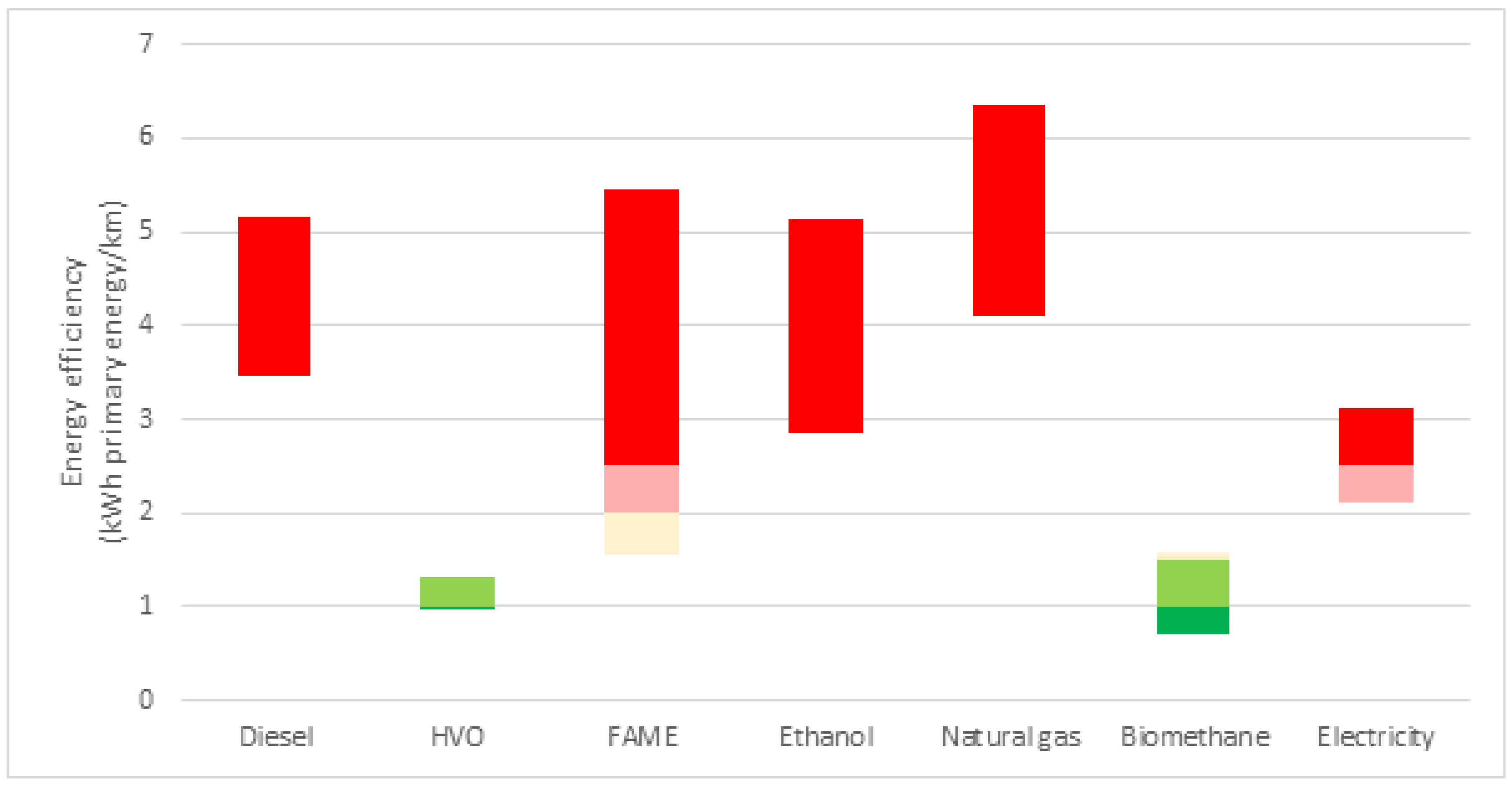
3.3.1. Non-Renewable Primary Energy Efficiency

Non-renewable primary energy efficiency comprises the amount of well-to-wheel primary energy use. The scale focuses on the amount of primary energy (kWh) per vehicle kilometer, based on the work of Gustafsson et al. [103]. However, the available data was too limited to make complete life-cycle estimations that also included the production of vehicles and infrastructure. The estimations thus deal with the energy efficiency in the fuel production and use of vehicles.
For diesel, the fuel production efficiency is in the range of 1.1–1.2 kWh primary energy/kWh fuel [104,105], while the vehicle efficiency (Vehicle efficiency in this section is the same as the fuel efficiency used in, for example, Section 3.2.1 Total cost of ownership and Section 3.3.2 Greenhouse gas emissions savings) corresponds to 3.2–4.1 kWh/km [28,46,50]. The combined result is Very Poor (Figure 3, Table 8).
HVO, FAME and ethanol all have the same vehicle efficiency as diesel buses. HVO, with a fuel production efficiency of 0.3 kWh primary energy/kWh from the mix of slaughterhouse waste and palm oil [104], could be either Good or Very Good. For FAME, there are fuel production efficiencies from 0.5 [104] to 1.3 kWh/kWh fuel [105], giving results ranging from Very Poor to Satisfactory. Ethanol is Very Poor due to a fuel production efficiency of between 0.9 and 1.3 kWh/kWh fuel based on a 50/50 mix of wheat [104,105] and maize [104].
Methane buses have a vehicle efficiency of 3.8–5.5 kWh/km [28,38,46,50]. Using natural gas gives a fuel production efficiency of 1.1–1.2 kWh/kWh fuel, corresponding to Very Poor. The fuel production efficiency, using biomethane from a mix of wastewater treatment sludge, manure and food waste, is 0.2–0.3 kWh/kWh fuel [104,105,106] and the resulting energy efficiency ranges from Satisfactory to Very Good.
Electric vehicles have the best vehicle efficiency of between 1.1 and 1.6 kWh/km [28,49,50]. But their performance is also influenced by the electricity production efficiency based on a mix of 40% nuclear power, 40% hydropower and 20% wind power, which is around 1.4 kWh/kWh fuel [105]. Apart from the efficiency of the vehicle, electric vehicles also need extra heating since the engine does not in itself generate heat that can be used. Previous experience of heating electric buses in Sweden [107] and temperature data from 1960–1990 [108] suggests that the yearly average of heating will be between 0.54 kWh/km in the warmest parts of Sweden and 1.1 kWh/km in its coldest parts. These heaters can use all the different diesel fuels, but it is assumed that HVO is used (which was also used in the buses that Jerksjö studied). Based on the fuel production efficiency of HVO, the heating adds from 0.17 to 0.35 kWh primary energy/km. In summary, this gives the result Very Poor or Poor.
There are both uncertainties regarding vehicle efficiency and fuel production efficiency. The vehicle efficiency differs depending upon the driving conditions: more hilly landscapes and more starts and stops require, for example, more energy. Different bus models also have slightly different energy efficiencies depending on, for example, the construction of the vehicle and the motor. For electric buses, there will also be added uncertainties of the vehicle efficiency due to the lack of maturity. Regarding fuel production efficiency, there will be differences in the production efficiency depending on, for example, the scale of the production plants, the technologies used in the production plants and so forth. Due to these uncertainties, all alternatives except diesel are assessed as **.
Other assumptions, or regional conditions, could yield significantly different results. If electricity production were only based on wind power (less than 0.1 kWh/kWh), electric buses would be lifted to the level Very Good, while 100% nuclear power (above 3 kWh/kWh) would mean Very Poor. For specific cases, it is recommended to use specific data/assessments.

3.3.2. Greenhouse Gas Emission Savings

The indicator of greenhouse gas emission savings is based on the total life cycle greenhouse gas emissions for each technology, which are compared to the corresponding emissions for diesel. The scale focuses on the emission savings in percent, with even steps in the range of 0–100%.
Diesel, estimated to emit 1241 g CO2-eq/vehicle km (based on emissions from [109]), is assessed as Very Poor (Table 9) since it, by definition, has 0% savings. HVO was estimated to have GHG emissions between 170 and 720 g/km (i.e., a savings of 29–84%), which corresponds to a range from Satisfactory to Very Good (Figure 4). These estimates include emissions from production (50% tallow oil and 50% palm oil) and use according to Börjesson et al. [52], Edwards et al. [104] and Prussi et al. [109] with the same fuel efficiencies as in Section 3.2.1. Similarly, FAME (based on rapeseed) was estimated to have emissions of around 200–900 g/km [52,104,105], corresponding to a savings of 29–84%, ranging from Poor to Very Good. Based on 50% maize and 50%, wheat ethanol was estimated to have GHG emissions of 540–1120 g/vehicle km [52,104,105,109], meaning savings of 9–56% and thus Very Poor to Satisfactory. Natural gas use emits 760–1460 g/km [104,105,109,110,111], giving up to 39% savings and thus is Very Poor to Poor. Biomethane, with 33% wastewater treatment sludge, 33% manure and 33% food waste, was estimated from 240–500 g/km [52,104,105,106,109], corresponding to savings from 81% up to above 100%, which is Very Good. Electric buses, based on 40% nuclear power, 40% hydropower and 20% wind power, were estimated to have emissions between 5 and 40 g/km [105,112,113], as well as 29–190 g/km (Based on the need for heating found by Jerksjö [107], temperature data from the Swedish Meteorological and Hydrological Institute [108] and on the emission data found for HVO [52,104,109]) of added emissions due to the use of HVO in heaters, corresponding to Very Good.
These literature-based estimations of GHG emissions vary considerably, especially for renewable fuels, and are therefore assessed to have medium certainty (**). The GHG emissions differ depending on the resource mix, characteristics of the production plants, transport distances, distribution and so forth. The assessment is based on assumptions corresponding to a Swedish context. Like the other indicators, the results would be different with other assumptions. For example, ethanol production only based on wheat straw would mean 90% lower GHG emissions [104], and there is ethanol produced in Sweden that is claimed to perform on this level [114]. On the contrary, ethanol based on 100% maize can have worse performance than fossil fuels [104]. Likewise, an EU or international electricity mix would lead to significantly worse results for electric buses [115].

3.3.3. Air Pollution

The indicator of air pollution regards emissions to air with a negative impact on health and the environment. The scale is primarily based on the definitions of low emission zones in Sweden and the Euro classifications for buses.
As the focus is on new buses, all alternatives should comply with the Euro VI requirements. However, for earlier versions of the Euro guidelines (Euro V and older), the emissions have been found to significantly exceed the standards’ limits in real-world driving [116,117]. The emissions have been especially high in connection with urban driving when the after-treatment needs to operate at lower engine temperatures [116,117,118,119], and during periods with cold outdoor temperatures [120]. Similar problems have been noted for Euro VI diesel buses [121,122,123], and these problems increase during periods with cold outdoor temperatures [120]. However, Euro VI vehicles seem to have significantly reduced overall emissions in contrast to older vehicles, also at lower road speeds, that is, in central city environments [121,123,124]. Thus, it seems like Euro VI diesel buses can range from Poor to Satisfactory (Table 10).
FAME appears to have lower emissions than diesel of, for example, particulate matter (PM), hydrocarbons and CO, while emissions of NOx are higher [125,126,127] (based on studies and modelling on Euro III-Euro VI buses). Liu et al. [125] found similar results for HVO—although the NOx emissions were above the level for diesel, they were not as high as for FAME. Buses that run on FAME and HVO may, similar to diesel, live up to Euro VI, but can sometimes have emissions at the Euro V level. They are thus assessed as either Poor or Satisfactory.
Regarding ethanol, no studies have been found on real-world driving emissions that focus on ED95 buses. However, a previous study on E85 Euro V-Euro VI buses found NOx and PM emissions to be lower than the emissions from diesel buses [126]. Since a major part of the fuel is the same (i.e., ethanol), ethanol is assessed as Satisfactory.
For methane-powered buses, that is, natural gas and biomethane, two previous studies found that NOx emissions are lower than for diesel buses ([119] (Euro V), [126] (Euro V-Euro VI)) and that the emissions did not increase as much when the average speed was less than 20 km/h [119]. PM emissions were also found to be lower than for diesel [118,126,128] as well as HC emissions [126]. For CO emissions, Chen et al. [118] found reduced emissions, while Moldanova et al. [126] found that emissions increased. Napolitano et al. [129] found that the emissions of particulate matter in SI Euro VI engines were within the prescribed limits. According to the scale of the indicator, both natural gas and biomethane are assessed as Good since they are driven by gas engines fulfilling the Euro VI requirements.
Due to the lack of studies on air pollution from real driving with new buses, and the sometimes-mixed results of different studies or with some pollutants having higher emissions and other lower emissions, all combustion engine alternatives have a high uncertainty (*).
Electric buses have no tailpipe emissions, but the electricity is assumed to be produced by 40% nuclear power, so they are thus assessed as Good.

3.3.4. Noise

The scale for the indicator of noise is based on the noise limits for new buses according to EU regulation 540/2014, which sets limits (in dBA) related to the engine power. This regulation, which became valid in 2016, included a stepwise sharpening with decreased limits in 2020 and 2024. The Satisfactory in the assessment scale corresponds to the 2016 limits, while Good and Very Good match the levels for 2020 and 2024, respectively. Very Poor and Poor were chosen with the same interval of dBA as the levels for Satisfactory and above.
As new buses (in EU) must comply with EU regulation 540/2014, all alternatives should reach the level of Good. The Swedish Transport Agency provided registered noise values for different bus models (Euro VI buses), including models for all the studied fuels with the exception of ethanol (no Euro VI 12-m ethanol bus was found) and electricity. Some models had noise levels just below the limit at the time, while others had registered noise levels that were several decibels quieter (Appendix B). The registered noise levels seemed more connected to the specific bus model than the type of fuel used.
However, previous research has found differences between some of the technologies. Noise differences are most obvious at lower speeds, as tire, road and wind noise even out the differences at higher speeds, and at bus stops [130,131,132]. Differences in noise between the alternatives are thus primarily affecting urban areas or the areas where buses start and stop. Laib et al. [130] found that buses have to represent at least 2% of the traffic flow in order for electric buses to make an impact on overall noise level on roads with heavy traffic. Thus, more silent buses may have a very limited impact on the overall noise levels on most roads, where other vehicles dominate.
In an older test with three buses (from 2012–2014), diesel-powered buses had an average acceleration noise corresponding from Satisfactory to Very Good [133] (Table 11). No studies were found on differences between the alternative fuels used in a diesel motor. HVO, FAME and ethanol are assumed to have the same noise levels as fossil diesel (i.e., Satisfactory to Very Good). Due to the lack of data found on tests of the real-world noise level of new buses, the uncertainty is assessed as high (*).
For methane-powered buses, previous studies provide a mixed picture. Several state that methane-powered heavy vehicles have lower noise levels than corresponding diesel vehicles [134,135,136,137], but some studies claim the opposite [131,133,138]. However, several of the studies are limited in that they use older buses than Euro VI and/or base the results on only a small number of vehicles. Natural gas and biomethane are both assessed as Satisfactory to Very Good, with a high uncertainty due to the mixed picture and to the lack of data on the real-world noise level of new buses.
For electric-powered buses, it is commonly found that they make much less noise than diesel at slower speeds [132,133,135,136,138,139,140]. Electric buses are assessed as Very Good.

3.3.5. Local/Regional Impact on Land and Aquatic Environments

The indicator of local/regional impact on land and aquatic environments deals with environmental impacts not covered by the other indicators by considering whether the total local/regional environmental impacts are positive or negative.
Diesel has negative local/regional impacts in that the production, and oil spills, can contaminate water and land [141,142] and negatively impact wildlife [143]. Diesel is linked to several significant negative local and/or regional environmental effects and is thus judged as Very Poor (Table 12).
The HVO used in Sweden 2018 was based on slaughterhouse waste, but also a significant share of PFAD [16], which since a few years back is re-classified by the Swedish Government as a co-product (not as waste anymore). Since PFAD comes from palm oil production, it is associated with effects such as deforestation of rainforests and biodiversity loss [144]. No environmental effects have been allocated from the animal production to the slaughterhouse waste (standard procedure, for wastes). HVO was found to be associated with a significantly negative local and/or regional environmental impact, with no significant positive effects, and is therefore judged as Very Poor. However, if the HVO was only based on slaughterhouse waste, the result would be Satisfactory. The governmental reclassification will likely lead to lowered use of PFAD in the coming years. All HVO made from PFAD must be traceable and meet biofuel sustainability criteria in order to be able to qualify for tax exemptions [144].
In line with our assumptions, FAME and ethanol are both based on cultivated crops—maize, wheat or rapeseed. Cultivated crops for energy purposes, such as ethanol and RME from conventional farming, often have negative impacts (such as eutrophication and acidification) on the local environments [145,146,147,148,149]. Common fertilization practices with mineral phosphorous can also cause increased levels of heavy metals in the soils [150]. Common agricultural practices also have negative effects on the land used, with a degradation of the land [150] as well as negative effects on biodiversity [148]. However, the by-products from both ethanol and FAME production can be used as protein-rich fodder for cattle, which can reduce the need for imported soy protein [151,152,153]. Soy products can negatively impact the local land where the soy is produced [154,155]. Thus, both ethanol and FAME are associated with significantly negative local and/or regional environmental impact associated with conventional farming, but the reduced impact linked to soy production leads to both FAME and ethanol being assessed as Poor.
Like diesel, natural gas production can be associated with significant negative local/regional impacts, such as the contamination of water [141,142]. As no positive environmental effects were found, it was judged as Very Poor.
Biogas is based on wastewater treatment sludge, manure and food waste according to the assumptions. When food waste or sewage sludge is digested and the digestate used as a fertilizer, nutrients are recycled [156,157,158,159]. This improves the local and regional nutrient supply and can reduce nutrient leakage in comparison with conventional fertilization practices [158,160]. Assuming that the manure would have been recycled anyway, biogas production does not increase the recirculation for that source. However, the digestion process positively influences the nutrient plant availability for manure and food waste [161], which is positive. Furthermore, anaerobic digestion of manure reduces problems of bad odors [162,163,164]—although the biogas plants themselves can have difficulties with bad odors [156]. The digestate returned to the fields has a lower amount of carbon [165], which may lead to relatively lower soil organic carbon levels in comparison with recycling without anaerobic digestion. However, studies have shown that the negative effects of using digested materials on soil fertility are low [165,166] or can even be positive due to more stabilized organic matter after the digestion [165]. To use digested wastewater treatment sludge as a fertilizer is politically contested in Sweden due to the risk of spreading substances that can have a negative impact [167]. Although there are, for example, metals, antibiotic-resistant genes and organic substances in the digested sludge that could have a negative effect, the same elements and compounds are found in fertilizers such as manure or in food waste [167]. Studies made on plants fertilized with digested sludge have not shown higher concentrations of those substances than for plants from other agricultural lands [167]. In summary, biogas solutions are associated with several positive local and regional environmental effects, with some negative (but still acceptable) effects, and is thus assessed as Good.
Three different energy sources were considered for electricity production—water, wind and nuclear power. Wind power development has negative local effects on both animals and humans via noise, visual impacts [168] and collisions [169]. Regarding hydropower (water), it has also been found that flora and fauna are negatively affected (e.g., [170]). Nuclear power is associated with potential risks for significant negative local, regional and international environmental effects [171]. It also uses radioactive materials that, like materials used in batteries in the vehicles, are mined in different ways—which causes a number of different negative local/regional environmental effects [171]. Nuclear power also produces radioactive waste [172], which has to be very carefully stored for thousands of years. Electric vehicles can also have negative local and regional impacts from battery production since there are often negative impacts from mining [173] (Although the battery production for electric buses is included, the production of the rest of the buses (including the production of the electric buses themselves) is not included since it is supposed to be the same for all of the alternatives). The management of used batteries from electric buses will likely also have local environmental effects. However, as no commercial scales of battery management exist yet, it is not clear what the effects will be. Electric buses are associated with significant negative local/regional environmental effects but no significant positive effects; they are thus judged as Very Poor.
The assessments for all biobased fuels and electricity have been assigned some uncertainty (**) due to the complexity of the production systems, making it difficult to correctly consider all local/regional environmental effects.
The results concerning local/regional impact on land and aquatic environments are very dependent on specific conditions. For example, biogas produced from energy crops, which is not common in Sweden, have similar negative impacts as those stressed for ethanol or FAME. On the other hand, all fuels based on energy crops would have better assessment results if the crops were produced by ecological farming, which is more favorable regarding biodiversity than conventional farming [174]. Thus, case-specific assessments are needed to provide an accurate picture for a particular context.

3.4. Social Performance

The indicators of energy security and employment and sociotechnical systems services were assessed to also cover some social performance.

3.4.1. Energy Security

The indicator of energy security focuses on where the production of the fuel or electricity takes place and the origin of the resources (such as feedstock for biofuels), considering geographical proximity.
No extraction of fossil fuels takes place in Sweden; they are imported [16]. During 2018, oil was primarily imported from Russia, Norway and Nigeria [16]. The refining of the oil to diesel is done almost exclusively in the EU—only 1–2% of the oil is refined outside the EU [16]. However, since the resources originate from outside of the EU, the assessment of diesel is Very Poor (Table 13).
Only 5% of the resources for HVO production originated from Sweden in 2018 [16]; the majority was imported from countries outside the EU. Indonesia, Malaysia and the USA accounted for more than 50% of the total production, while around 30% came from a number of other countries—including, for example, Russia, Uruguay, El Salvador, Gabon, Thailand and Vietnam [16]. Like diesel, HVO is thus assessed as Very Poor.
A majority of the resources for FAME used in Sweden in 2018 came from EU countries [16]. However, 10% came from Australia and 25% from other non-EU countries, including Russia, Bahrain, Taiwan and Kazakhstan [16]. FAME is thus also assessed as Very Poor.
For ethanol, all resources originated from within the EU during 2018, with 16% from Sweden [16]. Ethanol is assessed as Satisfactory.
Natural gas used in Sweden primarily comes from Denmark [175,176], but some gas is also imported as LNG from Norway [175]. No specific numbers could be found of exactly how much natural gas is imported from each country, but it is assumed that the share of the two neighboring countries is above 90% of the total imports. Natural gas is thus assessed as Satisfactory, but the uncertainty is judged as high due to the missing information (*).
The biogas sold in Sweden during 2018 came from both Sweden (71%) and Denmark (24%) [16], which provides the basis for the assessment Satisfactory.
According to the assumptions, 60% of the electricity is produced from renewable national wind and hydropower sources. However, the rest (40%) is assumed to be based on nuclear power, and the radioactive material used in nuclear plants is imported. No newly updated source could be found on where the nuclear fuel used in Sweden is mined, but older sources have stated countries like Australia, Canada, Namibia, Russia and Kazakhstan [177,178]. Electricity is thus assessed as Very Poor. Due to the age of the sources, the uncertainty is high (*).
The results regarding energy security are generic, applying a Swedish perspective. More specific considerations could give very different outcomes. For example, a large share of the biogas used in Sweden is based on local/regional sources and is locally produced and used [16]. There are more local/regional solutions for other technologies, such as electric solutions only based on local wind or solar power.

3.4.2. Sociotechnical System Services

The indicator of sociotechnical system services accounts for the public bus transport system’s impact on other sociotechnical systems, like the energy, water and waste management systems. It is considered whether each bus technology affects other sociotechnical systems positively or negatively.
Most of the bus technologies do not have any significant effects on any regional or municipal sociotechnical systems services, disregarding what has been covered by the other indicators (such as water pollution, etc.). This goes for diesel, FAME, HVO, ethanol and natural gas, all assessed as Satisfactory (Table 14).
For the included biogas solutions, there are, however, several positive links to sociotechnical systems [87]. For example, anaerobic digestion is an important treatment method for different types of waste that reduces waste volumes [151,179,180], stabilizes sewage sludge and reduces the amount of volatile compounds [180,181]. Biogas production can thus significantly facilitate the waste and wastewater management in a region/municipality and is thus assessed as Very Good.
Regarding electricity, battery electric vehicles can have some effect on the local grid via how the vehicles are used. If a large number of buses in a city need fast recharging during the day, there can be significant problems with effect peaks and the infrastructure for the electricity system. However, if the vehicles charge when there is low demand, for example, overnight, it can reduce the peak needed in the system [182] and thus the impact on the system. It can even be beneficial to the system to have plug-in vehicles charging at hours with otherwise low electricity consumption as it can even out the peaks that already exist and thus enable a more even production [183], as well as using a surplus of renewable electricity generation [184]. Electricity is assessed as Very Poor to Good.

4. Concluding Discussion

Researchers within the field of sustainability assessment emphasize the need to better integrate sustainability into central decision-making processes [185,186]. Well-managed GoSPP constitutes a great opportunity [187,188], but there is a need for guidelines and supportive tools [188,189,190,191]. We have established an MCA method for broad assessments of bus technologies’ sustainability, focusing on a regional public procurement context. The ongoing development of transport technologies demands regular sustainability assessments (including the development of suitable methods). As exemplified by this study, the introduction of electric vehicles, new gas engines, the rapid shift to HVO and the relatively novel use of ethanol are all examples that motivate continuous work with assessments.
In the first article (Part I), the MCA method is established and discussed in relation to criteria regarding effective and efficient sustainability assessments. In this concluding discussion, we start by discussing the overarching results from having applied the MCA method on the selected bus technologies, focusing on Swedish conditions but also, to some extent, local/regional and international perspectives. We also continue the discussion in Part I by then problematizing the MCA method’s usefulness for practitioners and its accuracy from a scientific perspective.

4.1. Discussion of the Assessment Results

Table 15 provides an overview of the assessment results. Generally, the alternatives using diesel engines have the best technical scores. The gas engines also perform well, while the electric vehicles have a lower technical maturity. For all the technical indicators, the level of uncertainty was low (***).
The picture is relatively scattered concerning the economic performance, and the level of certainty significantly lower. Starting with TCO, the literature contained data ranging over 3–5 levels for most of the alternatives due to, for example, different possible fuel efficiencies and purchase costs. For all the diesel fuels and electricity, there were reported costs on the level of Very Good, but HVO and electricity could also be Very Poor. Biomethane and natural gas vehicles may be Good, but data that would bring them down to the lowest level were also found. For ethanol, the little data found only reached the two lower scores, mainly due to relatively high costs for fuel and maintenance. Even though it is difficult to draw definite conclusions regarding the cost stability, the expected high demand and limited raw material base indicate especially high risks of increased costs for HVO. Regarding the need for investments in infrastructure, all the alternatives require significant investments (Very Poor). However, this is not indicated in Table 15, as the main point is to make case-specific assessments and then consider existing infrastructure (that new alternatives may be more expensive). It should be noted that the economic indicators are focused on the “procurement budget” and costs related to infrastructure, that is, a relatively narrow scope. To better understand the socioeconomic implications, one also needs to consider the environmental and social performance.
When considering the environmental dimension, fossil fuels are, as expected (and for some indicators directly based on their definition) and supported by many other studies (e.g., [192,193]), clearly non-sustainable alternatives. They are linked to many negative impacts, although natural gas sometimes performs a bit less poorly than diesel. All the renewable alternatives can contribute importantly towards improved sustainability if they are smartly produced, used and combined [194,195]. Among the renewable alternatives, HVO and biomethane have the highest non-renewable primary energy efficiencies. Biomethane outperforms the others from a generic environmental perspective, and more specifically, being the only option able to provide negative GHG emission levels. However, electric vehicles can be favorable in central city areas due to their low noise levels and as there are no local exhausts emissions, and given the technology’s energy efficiency benefits are most relevant in city areas. It should be emphasized that environmental performance is very dependent on the underlying sociotechnical and agricultural systems. Renewable and waste-based systems commonly perform very well [15,196]. Applying a marginal perspective on electricity, which may be reasonable in Northern Europe, would lead to far worse results for electric buses [197]. Ecological farming would strengthen the results for the crop-based fuels, as they are pulled down by conventional farming with non-sustainable links to mineral fertilizers and pesticides [174,198,199]. The level of certainty varied substantially for the environmental indicators.
Regarding social performance, biomethane comes out best due to positive links to other sociotechnical systems and energy supply services. Electric buses can both bring positive and negative effects. Regarding energy security, biogas, natural gas and ethanol all scored on the Satisfactory level, with the rest being considered Very Poor. Generally, there was a low level of uncertainty (***), with the exception of natural gas and electricity in the indicator Energy security, due to lack of recent data.

4.2. Usability and Accuracy

In addition to the assessment results, testing the MCA method on seven bus technologies brought interesting observations and questions. On an overarching level, a majority of the indicators worked relatively well, meaning that they provided usable questions and scales for assessment, and we found matching data. For those indicators, the assessment was fairly straightforward.
However, data from many different studies and the focus on the Swedish market, in general, led to a wide range of values for several indicators and technologies. This largely explains the scattered picture in Table 15, which makes it difficult to conclude what alternative is best, although much interesting information is provided. If the MCA method, as intended, is used for a particular public procurement, it would be possible to use specific data for each technology (or tender for each actor), which would provide more clear-cut answers with a higher level of certainty. This is not only true for more quantitative indicators like total cost of ownership, but also for more qualitative indicators like cost stability—for example, due to fixed price agreements or insurances.
While some indicators seemed fairly well defined, it was challenging to find trustworthy data. For both the indicators noise and air pollution, there seems to be a lack of studies looking at real-life conditions of new Euro VI buses. Thus, it is uncertain to what extent registered values on noise and air pollution are actually correct, not least as the transport sector historically has used many test values with significantly underestimated impacts [200,201].
In addition, a few indicators were more difficult to assess, both related to their definition and information availability. Cost stability has the inherent challenge of estimating future costs, which is very complicated. Furthermore, the indicator local/regional impact on land and aquatic environments includes a wide range of different impacts that commonly vary due to local conditions, for example, where and how a fuel is produced, making it more difficult to conduct well-based assessments. The qualitative character of these two indicators also complicates the assessment. However, the assessment was not experienced as difficult for all qualitative indicators. To include qualitative indicators is imperative for focusing on essential issues rather than only on what can be easily measured or quantified [186,202]. Documentation and references are essential for all the assessment results to ensure transparency, but the qualitative indicators may require extra careful motivations in relation to the terms of the scales. Our ambition has been to establish scales that are easy to understand, but linguistic imprecisions leave room for interpretations to assessors—for example, in specific cases to decide what is considered to be “minor” or “significant” investments.
For quantitative scales, using numbers may indicate a higher certainty than is the case. To reduce this problem, we have used intervals when relevant, instead of answering with a single number, and indicated the level of uncertainty.
Despite all the challenges and opportunities to provide more specific results, we have established an MCA tool that could be used to support public procurement processes. It is challenging to establish a sustainability assessment method that is both broad and simple, as requested [14]. The MCA method is based on 12 sustainability indicators of relevance for all technologies, selected based on literature reviews and stakeholder input, to balance these diverging needs. Although several other studies using MCA have included a similar number of indicators, or even more [203], this is a broad stance from the perspective of GoSPP [15]—the MCA method can contribute towards broadened GoSPP. The developed MCA method can importantly contribute to improved knowledge on the sustainability of different bus technologies, as it helps in structuring relevant information, thereby facilitating overview and more informed decision making.

4.3. Future Research

It would be fruitful to study actual cases where the method is used to support public procurement in different ways (improved knowledge, formulation of requirements, etc.) to learn more about the MCA method’s usability and how to further develop it. As the method has been developed and applied in a Swedish context, it would be interesting to learn from adaptions to other contexts and assessments there, for example in other countries outside EU. Another opportunity would be to study a certain bus model to be used in different parts of the world to see how the sustainability of a certain technology varies between different geographical regions. The method can also be used to study different versions of a fuel, for example, to indicate the importance of different types of biomass/feedstock, underlying farming systems and local versus international production. There are also other bus technologies that could be studied, such as buses using hydrogen or hybrid buses. The MCA method can also be developed to address similar decision-making challenges. For example, heavy-duty trucks have many similarities with buses, and only minor changes to the method might be needed to assess such vehicles.

Author Contributions

Conceptualization, S.D. and J.A.; methodology, S.D. and J.A.; validation, S.D. and J.A.; formal analysis, S.D. and J.A.; investigation, S.D. and J.A.; writing—original draft preparation, S.D. and J.A.; writing—review and editing, S.D. and J.A.; visualization, S.D. and J.A.; supervision, S.D. and J.A.; project administration, S.D. and J.A.; funding acquisition, J.A. All authors have read and agreed to the published version of the manuscript.

Funding

This research was performed within the Biogas Research Center (BRC), which is funded by the Energy Agency of Sweden, Linköping University and the Swedish University of Agriculture, and more than 20 private and public partners.

Institutional Review Board Statement

Not applicable.

Informed Consent Statement

Not applicable.

Data Availability Statement

The data presented in this study are available on request from the corresponding author. The data are not publicly available due to privacy.

Acknowledgments

We want to thank the five students who, during 2018, contributed to this project—Jacob Dahlstedt, Agnes Lundgren, Éamon Magorrian, Linnea Orsholm, and Anders Wilzén. We are also very grateful for the input from participants, stakeholders, and reviewers.

Conflicts of Interest

The authors declare no conflict of interest.

Appendix A

Table A1. Actors that have been involved in the MCA method development process, more actively as participants (P) in research projects, and stakeholders (S) that have been given the opportunity to provide input at meetings and conferences.
Project Participants (P, p (a Capital Letter Indicates Participation through the Whole MCA Method Establishment Process or a Large Contribution in Any Stage, while a Lowercase Letter Indicates a Smaller Contribution, Often in the Later Stages)) and Involved Stakeholders (S)Relevance, CompetencesComment
Region Östergötland (P), part in BRCEnvironmental strategist with long term experience regarding bus technologies, sustainability issues and public procurement processesHas participated in the whole MCA establishment process and has been part of several workshops to establish what indicators and scales can be relevant for assessing bus technologies. The region is the case of study
Other regions (p)Long-term experience regarding public bus transports and other relevant issuesThe regions of Gotland, Kalmar and Jönköping participated in later stages of the process (the last two years). They, e.g., provided input at a dedicated workshop
Gasum (P), part in BRCRepresented by a business development specialist and a civil engineer specialized in environmental and energy management. Also represented by a business development managerParticipated in the whole MCA establishment process and has been part of several workshops to establish what indicators and scales can be relevant for assessing bus technologies
Linköping University (P, p), part in BRCExperts in:
-environmental systems analysis and biofuels (P)
-business administration (p)
-socio-technical systems (p)
Four researchers participated through the whole MCA establishment process, the authors and two other colleagues. Researchers with expertise in business administration and socio-technical systems provided input in later stages
Municipalities (p), part in BRCLong term experience regarding public bus transports and other relevant issuesThe municipalities of Linköping and Norrköping participated in later stages of the MCA establishment process (the last year) They, e.g., provided input at a dedicated workshop
Tekniska Verken (p), part in BRCA municipally owned utility company, e.g., with expertise in energy and waste management. Long-term experience in biogas production and use for public bus transportsProvided input at the later stages of the MCA establishment process (the last year)
Scania (p), part in BRCThis company provides transport solutions. Manufacturer of buses and trucks, with expertise regarding all the studied vehicle types and fuelsProvided input at the later stages of the MCA establishment process (the last year). They, e.g., provided input at a dedicated workshop
Borlänge energi (p), part in BRCA municipally owned utility company, e.g., with expertise in energy and waste management. Experience in biogas production and use for public bus transportsThey provided input at a dedicated workshop
JES (S)A management consultancy firm that has been working with, e.g., biogas and public transportThey provided input at a dedicated workshop
Vattenfall (S)A state-owned energy utility company operating in Europe. E.g. expertise in electrificationTook part in a research project called “Miljöbuss”, in which the authors participated. Provided input in relation to two presentations of the MCA method
Other partners of BRC (S)Other than the already listed organizations taking part in this transdisciplinary research center. Expertise within many areas related to socio-technical systems, fuels, transport, etc. The project and MCA method were presented at large BRC meetings during poster sessions, which resulted in relevant input from people with different backgrounds and competences
Table A2. Competences of actors involved in reviewing the articles in the final stages of the process.
Competence Areas of Actors
Sustainability systems analysis
-
Multi-Criteria Assessment
-
Life Cycle Analysis
-
Life Cycle Costing
-
Energy Analysis
Transportation
-
Especially regarding other fuels than biomethane to complement the competency profile of the authors
Sociotechnical systems
-
Especially in connection to the indicator sociotechnical system services
Environmental innovations
-
Especially in connection to the indicators of technical maturity and cost stability

Appendix B

Table A3. The Swedish Transportation Agency database on registered vehicles was used to check examples of registered values of 12-m Euro VI buses. The buses found were all registered between 2017 and 2019.
BrandModelTechnologyMotorNoise
BYDEbusElectricity250 kW71 dB
MANLion’s CityMethane228 kW77 dB
Mercedes-BenzCitaroMethane222 kW73 dB
Mercedes-BenzEcitaroElectricity252 kW72 dB
ScaniaCitywideDiesel235 kW77 dB
ScaniaCitywideMethane235 kW77 dB
ScaniaCitywideElectricity210/290 kW77 dB
Volvo7900Electricity186 kW67 dB
Volvo8900Diesel/Biodiesel240 kW73 dB
Volvo9700Diesel285 kW76 dB

References

  1. Banister, D.; Button, K. Transport, the Environment and Sustainable Development; Routledge: Oxfordshire, UK, 2015; ISBN 978-1-135-15517-9. [Google Scholar]
  2. Sims, R.; Schaeffer, R.; Creutzig, F.; Cruz-Núñez, X.; D’Agosto, M.; Dimitriu, D.; Figueroa Meza, M.J.; Fulton, L.; Kobayashi, S.; Lah, O.; et al. Transport. In Climate Change 2014: Mitication of Climate Change. Contribution of Working Group III fo the Fifth Assessment Report of the Intergovernmental Panel on Climate Change; Cambridge University Press: Cambridge, UK; New York, NY, USA, 2014. [Google Scholar]
  3. Anenberg, S.; Miller, J.; Henze, D.; Minjares, R. A Global Snapshot of the Air Pollution-Related Health Impacts of Transportation Sector Emissions in 2010 and 2015; The International Council on Clean Transportation: Washington, DC, USA, 2019; p. 55. [Google Scholar]
  4. Xia, T.; Nitschke, M.; Zhang, Y.; Shah, P.; Crabb, S.; Hansen, A. Traffic-Related Air Pollution and Health Co-Benefits of Alternative Transport in Adelaide, South Australia. Environ. Int. 2015, 74, 281–290. [Google Scholar] [CrossRef]
  5. Braubach, M.; Tobollik, M.; Mudu, P.; Hiscock, R.; Chapizanis, D.; Sarigiannis, D.A.; Keuken, M.; Perez, L.; Martuzzi, M. Development of a Quantitative Methodology to Assess the Impacts of Urban Transport Interventions and Related Noise on Well-Being. Int. J. Environ. Res. Public Health 2015, 12, 5792–5814. [Google Scholar] [CrossRef] [PubMed] [Green Version]
  6. Lercher, P. Noise in Cities: Urban and Transport Planning Determinants and Health in Cities. In Integrating Human Health into Urban and Transport Planning: A Framework; Nieuwenhuijsen, M., Khreis, H., Eds.; Springer International Publishing: Cham, Switzerland, 2019; pp. 443–481. ISBN 978-3-319-74983-9. [Google Scholar]
  7. Li, T.; Shilling, F.; Thorne, J.; Li, F.; Schott, H.; Boynton, R.; Berry, A.M. Fragmentation of China’s Landscape by Roads and Urban Areas. Landsc. Ecol. 2010, 25, 839–853. [Google Scholar] [CrossRef] [Green Version]
  8. Shannon, G.; Angeloni, L.M.; Wittemyer, G.; Fristrup, K.M.; Crooks, K.R. Road Traffic Noise Modifies Behaviour of a Keystone Species. Anim. Behav. 2014, 94, 135–141. [Google Scholar] [CrossRef]
  9. Danielsen, F.; Beukema, H.; Br, C.A.; Reijnders, L.; Struebig, M. Biofuel Plantations on Forested Lands: Double Jeopardy for Biodiversity and Climate. Conserv. Biol. 2009, 23, 12. [Google Scholar] [CrossRef]
  10. Xylia, M.; Silveira, S. On the Road to Fossil-Free Public Transport: The Case of Swedish Bus Fleets. Energy Policy 2017, 100, 397–412. [Google Scholar] [CrossRef] [Green Version]
  11. Cheng, W.; Appolloni, A.; D’Amato, A.; Zhu, Q. Green Public Procurement, Missing Concepts and Future Trends—A Critical Review. J. Clean. Prod. 2018, 176, 770–784. [Google Scholar] [CrossRef]
  12. Testa, F.; Annunziata, E.; Iraldo, F.; Frey, M. Drawbacks and Opportunities of Green Public Procurement: An Effective Tool for Sustainable Production. J. Clean. Prod. 2016, 112, 1893–1900. [Google Scholar] [CrossRef]
  13. von Oelreich, K.; Philp, M. Green Procurement: A Tool for Achieving National Environmental Objectives (Translated); Swedish EPA: Stockholm, Sweden, 2013.
  14. Hüging, H.; Glensor, K.; Lah, O. Need for a Holistic Assessment of Urban Mobility Measures–Review of Existing Methods and Design of a Simplified Approach. Transp. Res. Procedia 2014, 4, 3–13. [Google Scholar] [CrossRef] [Green Version]
  15. Lindfors, A.; Ammenberg, J. Using National Environmental Objectives in Green Public Procurement: Method Development and Application on Transport Procurement in Sweden. J. Clean. Prod. 2020, 124821. [Google Scholar] [CrossRef]
  16. Swedish Energy Agency. Drivmedel 2018; Swedish Energy Agency: Eskilstuna, Sweden, 2019.
  17. Swedish Energy Agency. Energiläget i Siffror 2019; Swedish Energy Agency: Eskilstuna, Sweden, 2019.
  18. Fridas Användarförening FRIDA Miljö-Och Fordonsdatabas. Available online: http://www.frida.port.se/hemsidan/default.cfm (accessed on 12 February 2020).
  19. Statistics Sweden Fordonsbestånd 2018 [Vehicle Stock 2018]. 2019. Available online: https://www.scb.se/contentassets/4bf97f768344433f85bd81fcf0ce9b7b/fordon_2018_20200311.xlsx (accessed on 12 February 2020).
  20. Trafikanalys. Lokal Och Regional Kollektivtrafik 2009; Trafikanalys: Stockholm, Sweden, 2010; p. 82. [Google Scholar]
  21. International Association of Public Transport Global Bus Survey. Available online: https://www.uitp.org/sites/default/files/cck-focus-papers-files/Statistics%20Brief_Global%20bus%20survey%20%28003%29.pdf (accessed on 6 February 2020).
  22. UNECE New Vehicle Registrations by Fuel Type, Type of Vehicle, Country and Year. Available online: https://w3.unece.org/PXWeb2015/pxweb/en/STAT/STAT__40-TRTRANS__03-TRRoadFleet/08_en_TRRoadNewVehF_r.px/table/tableViewLayout1/ (accessed on 22 April 2020).
  23. Bloomberg New Energy Finance Electric Vehicle Outlook 2020. Available online: https://bnef.turtl.co/story/evo-2020/ (accessed on 28 May 2020).
  24. Sustainable Bus. Electric Bus, Main Fleets and Projects around the World 2019. Available online: https://www.sustainable-bus.com/electric-bus/electric-bus-public-transport-main-fleets-projects-around-world/ (accessed on 12 February 2020).
  25. Swedish Petroleum and Biofuel Institute. Utlevererad Volym Av Drivmedel 2020. Available online: https://www.petrolplaza.com/organisations/937 (accessed on 28 May 2020).
  26. Scarlat, N.; Dallemand, J.-F.; Fahl, F. Biogas: Developments and Perspectives in Europe. Renew. Energy 2018, 129, 457–472. [Google Scholar] [CrossRef]
  27. Vassileva, I.; Campillo, J. Adoption Barriers for Electric Vehicles: Experiences from Early Adopters in Sweden. Energy 2017, 120, 632–641. [Google Scholar] [CrossRef]
  28. Civitas. Smart Choices for Cities: Alternative Fuel Buses; Civitas: Brussels, Belgium, 2016. [Google Scholar]
  29. Lindgren, L. Electrification of City Bus. Traffic—A Simulation Study Based on Data from Linköping; Department of Industrial Electrical Engineering and Automation, Lund Institute of Technology: Lund, Sweden, 2017. [Google Scholar]
  30. Ally, J.; Pryor, T. Life-Cycle Assessment of Diesel, Natural Gas and Hydrogen Fuel Cell Bus Transportation Systems. J. Power Sources 2007, 170, 401–411. [Google Scholar] [CrossRef] [Green Version]
  31. Caban, J.; Ignaciuk, P. Technical-Economic Aspects of CNG Gas Usage in Buses of Urban Communication. In Proceedings of the 17 International Scientific Conference “Engineering For Rural Development”, Jelgava, Latvia, 23–25 May 2018. [Google Scholar]
  32. Lajunen, A.; Lipman, T. Lifecycle Cost Assessment and Carbon Dioxide Emissions of Diesel, Natural Gas, Hybrid Electric, Fuel Cell Hybrid and Electric Transit Buses. Energy 2016, 106, 329–342. [Google Scholar] [CrossRef]
  33. Stempien, J.P.; Chan, S.H. Comparative Study of Fuel Cell, Battery and Hybrid Buses for Renewable Energy Constrained Areas. J. Power Source 2017, 340, 347–355. [Google Scholar] [CrossRef]
  34. Sweco. Innovative Biogas Fuelling System Alternatives for Buses; Baltic Biogas Bus: Bergen, Norway, 2012. [Google Scholar]
  35. Aldenius, M.; Khan, J.; Nikoleris, A. Elektrifiering av stadsbussar: En Genomgång av Erfarenheter i Sverige Och Europa; K2-Sveriges nationella centrum för forskning och utbildning om kollektivtrafik: Lund, Sweden, 2016; p. 66. [Google Scholar]
  36. Borén, S.; Nurhadi, L.; Ny, H.; Andersson, M.; Nilsson, S.; Lööf, J. GreenCharge—Demotest i Fält Med. Elbuss; Blekinge Tekniska Högskola: Karlskrona, Sweden, 2015. [Google Scholar]
  37. Ahmadi Moghaddam, E.; Ahlgren, S.; Hulteberg, C.; Nordberg, Å. Energy Balance and Global Warming Potential of Biogas-Based Fuels from a Life Cycle Perspective. Fuel Process. Technol. 2015, 132, 74–82. [Google Scholar] [CrossRef]
  38. Ecotraffic. Kunskapssammanställning—Stadsbussar Euro VI. 2015. Available online: http://www.ecotraffic.se/media/13180/kunskapspm-euro_vi-bussar_-g_teborg_20_nov_2015.pdf (accessed on 12 February 2020).
  39. Guslén, B. Volvo Bussar har fått stororder. Göteborgs-Posten, 29 April 2015. [Google Scholar]
  40. Harris, A.; Soban, D.; Smyth, B.M.; Best, R. Assessing Life Cycle Impacts and the Risk and Uncertainty of Alternative Bus Technologies. Renew. Sustain. Energy Rev. 2018, 97, 569–579. [Google Scholar] [CrossRef] [Green Version]
  41. Lundström, A.-C.; Ninasdotter Holmström, M.; Torstensson, E.; Eriksson, M. Elbussar i Sveriges Kollektivtrafik—En Kartläggning av Trafikförvaltningen Stockholm, Skånetrafiken och Västtrafik Utifrån Fyra Perspektiv; Trafikverket: Solna, Sweden, 2019; p. 132.
  42. Mahmoud, M.; Garnett, R.; Ferguson, M.; Kanaroglou, P. Electric Buses: A Review of Alternative Powertrains. Renew. Sustain. Energy Rev. 2016, 62, 673–684. [Google Scholar] [CrossRef]
  43. Laizāns, A.; Graurs, I.; Rubenis, A.; Utehin, G. Economic Viability of Electric Public Busses: Regional Perspective. Procedia Eng. 2016, 134, 316–321. [Google Scholar] [CrossRef] [Green Version]
  44. Rogge, M.; van der Hurk, E.; Larsen, A.; Sauer, D.U. Electric Bus Fleet Size and Mix Problem with Optimization of Charging Infrastructure. Appl. Energy 2018, 211, 282–295. [Google Scholar] [CrossRef] [Green Version]
  45. Topal, O.; Nakir, İ. Total Cost of Ownership Based Economic Analysis of Diesel, CNG and Electric Bus Concepts for the Public Transport in Istanbul City. Energies 2018, 11, 2369. [Google Scholar] [CrossRef] [Green Version]
  46. Dyr, T.; Misiurski, P.; Ziółkowska, K. Costs and Benefits of Using Buses Fuelled by Natural Gas in Public Transport. J. Clean. Prod. 2019, 225, 1134–1146. [Google Scholar] [CrossRef]
  47. Scania. Scania E-Mail Conversation with Senior Engineer at Scania; Scania: Södertälje, Sweden, 2018. [Google Scholar]
  48. Eudy, L.; Jeffers, M. Foothill Transit Agency Battery Electric Bus Progress Report Data Period Focus: Jan. 2019 through Jun. 2019. Available online: https://www.osti.gov/biblio/1573208-foothill-transit-agency-battery-electric-bus-progress-report-data-period-focus-jan-through-jun (accessed on 12 February 2020).
  49. Tong, F.; Hendrickson, C.; Biehler, A.; Jaramillo, P.; Seki, S. Life Cycle Ownership Cost and Environmental Externality of Alternative Fuel Options for Transit Buses. Transp. Res. Part Transp. Environ. 2017, 57, 287–302. [Google Scholar] [CrossRef]
  50. DahlÖberg, J.; Vehabovic, A. Well-to-Wheel Greenhouse Gas Emissions of Heavy-Duty Vehicles Using Different Energy Carriers—Dependent on Electricity Carbon Intensity and Vehicle Applications. Master’s Thesis, Linköping University, Linköping, Sweden, 2018. [Google Scholar]
  51. Swedish Energy Agency Elbusspremie. Available online: https://www.energimyndigheten.se/klimat--miljo/transporter/transporteffektivt-samhalle/elbusspremie/ (accessed on 13 February 2020).
  52. Börjesson, P.; Lundgren, J.; Ahlgren, S.; Nyström, I. Dagens Och Framtidens Hållbara Biodrivmedel—I Sammandrag. Rapport f3. 18 June 2013, p. 209. Available online: https://www.energimyndigheten.se/globalassets/klimat--miljo/transporter/oppet-forum/f3/sammandrag_hallbara-biodrivmedel_160512.pdf (accessed on 25 January 2021).
  53. Smith, M.; Gonzales, J. Costs Associated with Compressed Natural Gas Vehicle Fueling Infrastructure; Technical Report DOE/GO-102014-4471; National Renewable Energy Lab. (NREL): Golden, CO, USA, 2014.
  54. Chen, Z.; Yin, Y.; Song, Z. A Cost-Competitiveness Analysis of Charging Infrastructure for Electric Bus Operations. Transp. Res. Part C Emerg. Technol. 2018, 93, 351–366. [Google Scholar] [CrossRef]
  55. Kunith, A.; Mendelevitch, R.; Goehlich, D. Electrification of a City Bus Network—An Optimization Model for Cost-Effective Placing of Charging Infrastructure and Battery Sizing of Fast-Charging Electric Bus Systems. Int. J. Sustain. Transp. 2017, 11, 707–720. [Google Scholar] [CrossRef] [Green Version]
  56. Bai, Y.; Okullo, S.J. Understanding Oil Scarcity through Drilling Activity. Energy Econ. 2018, 69, 261–269. [Google Scholar] [CrossRef]
  57. Banerjee, R.; Benson, S.M.; Bouille, D.H.; Brew-Hammond, A.; Cherp, A.; Coelho, S.T.; Emberson, L.; Figueroa, M.J.; Grubler, A.; Jaccard, M.; et al. Global Energy Assessment; Cambridge University Press: Cambridge, UK; New York, NY, USA; International Institute for Applied Systems Analysis: Laxenburg, Austria, 2012; p. 1865. [Google Scholar]
  58. Haugom, E.; Mydland, Ø.; Pichler, A. Long Term Oil Prices. Energy Econ. 2016, 58, 84–94. [Google Scholar] [CrossRef]
  59. Arzaghi, E.; Abbassi, R.; Garaniya, V.; Binns, J.; Khan, F. An Ecological Risk Assessment Model for Arctic Oil Spills from a Subsea Pipeline. Mar. Pollut. Bull. 2018, 135, 1117–1127. [Google Scholar] [CrossRef]
  60. Suprenand, P.M.; Hoover, C.; Ainsworth, C.H.; Dornberger, L.N.; Johnson, C.J. Preparing for the Inevitable: Ecological and Indigenous Community Impacts of Oil Spill-Related Mortality in the United States’ Arctic Marine Ecosystem. In Scenarios and Responses to Future Deep Oil Spills: Fighting the Next War; Murawski, S.A., Ainsworth, C.H., Gilbert, S., Hollander, D.J., Paris, C.B., Schlüter, M., Wetzel, D.L., Eds.; Springer International Publishing: Cham, Switzerland, 2020; pp. 470–493. ISBN 978-3-030-12963-7. [Google Scholar]
  61. Caldara, D.; Cavallo, M.; Iacoviello, M. Oil Price Elasticities and Oil Price Fluctuations. J. Monet. Econ. 2019, 103, 1–20. [Google Scholar] [CrossRef] [Green Version]
  62. Swedish Petroleum and Biofuel Institute. Diesel—Priser Och Skatter; SPBI: Stockholm, Sweden, 2020. [Google Scholar]
  63. European Commission 2030 Climate & Energy Framework. Available online: https://ec.europa.eu/clima/policies/strategies/2030_en (accessed on 27 February 2020).
  64. Swedish Environmental Protection Agency Sveriges Klimatmål Och Klimatpolitiska Ramverk. Available online: https://www.naturvardsverket.se/Miljoarbete-i-samhallet/Miljoarbete-i-Sverige/Uppdelat-efter-omrade/Klimat/Sveriges-klimatlag-och-klimatpolitiska-ramverk/ (accessed on 27 February 2020).
  65. Kallis, G.; Sager, J. Oil and the Economy: A Systematic Review of the Literature for Ecological Economists. Ecol. Econ. 2017, 131, 561–571. [Google Scholar] [CrossRef] [Green Version]
  66. Swedish Petroleum and Biofuel Institute SPBI Branschfakta 2019. Available online: https://spbi.se/wp-content/uploads/2019/07/SPBI_branschfakta_2019_DIGITAL-online1.pdf (accessed on 2 June 2020).
  67. Hjort, A.; Hansson, J.; Lönnqvist, T.; Nilsson, J. Utsikt För Förnybar Flytande Metan i Sverige till År 2030; f3. 2019. Available online: https://f3centre.se/app/uploads/f3-2019-05_Hjort-et-al-FINAL-191204.pdf (accessed on 3 June 2020).
  68. OKQ8 Prishistorik Företag 2020. Available online: https://www.okq8.se/~/media/dokument-foretag/drivmedel/prishistorik-foretag_2.xlsx (accessed on 2 June 2020).
  69. Weimar, A. HVO Kan få en Prislapp på 27 Kronor per Liter. Available online: https://www.atl.nu/entreprenad/hvo-kan-fa-en-prislapp-pa-27-kronor-per-liter/ (accessed on 3 June 2020).
  70. Swedish Petroleum and Biofuel Institute Skatter Förnybara Drivmedel 2020. Available online: https://spbi.se/statistik/skatter/skatter-fornybara-drivmedel/ (accessed on 28 February 2020).
  71. Swedish Tax Agency Ändrade Bestämmelser om Skattebefrielse för Biodrivmedel. Available online: https://www.skatteverket.se/foretagochorganisationer/skatter/punktskatter/energiskatter/energiskatterpabranslen/skattebefrielseforbiodrivmedel.4.2b543913a42158acf800021393.html (accessed on 28 February 2020).
  72. European Commission Sustainability Criteria for Biofuels Specified. Available online: https://ec.europa.eu/commission/presscorner/detail/en/MEMO_19_1656 (accessed on 3 June 2020).
  73. European Commission Renewable Energy—Recast to 2030 (RED II). Available online: https://ec.europa.eu/jrc/en/jec/renewable-energy-recast-2030-red-ii (accessed on 3 June 2020).
  74. Wang, Q.; Chen, X.; Jha, A.N.; Rogers, H. Natural Gas from Shale Formation—The Evolution, Evidences and Challenges of Shale Gas Revolution in United States. Renew. Sustain. Energy Rev. 2014, 30, 1–28. [Google Scholar] [CrossRef]
  75. Šebalj, D.; Mesarić, J.; Dujak, D. Predicting Natural Gas Consumption—A Literature Review. In Proceedings of the 28th International Conference “Central European Conference on Information and Intelligent Systems”, Varazdin, Croatia, 27–29 September 2017. [Google Scholar]
  76. Kan, S.Y.; Chen, B.; Wu, X.F.; Chen, Z.M.; Chen, G.Q. Natural Gas Overview for World Economy: From Primary Supply to Final Demand via Global Supply Chains. Energy Policy 2019, 124, 215–225. [Google Scholar] [CrossRef]
  77. Mouette, D.; Machado, P.G.; Fraga, D.; Peyerl, D.; Borges, R.R.; Brito, T.L.F.; Shimomaebara, L.A.; dos Santos, E.M. Costs and Emissions Assessment of a Blue Corridor in a Brazilian Reality: The Use of Liquefied Natural Gas in the Transport Sector. Sci. Total Environ. 2019, 668, 1104–1116. [Google Scholar] [CrossRef] [PubMed]
  78. Pfoser, S.; Aschauer, G.; Simmer, L.; Schauer, O. Facilitating the Implementation of LNG as an Alternative Fuel Technology in Landlocked Europe: A Study from Austria. Res. Transp. Bus. Manag. 2016, 18, 77–84. [Google Scholar] [CrossRef]
  79. Thomson, H.; Corbett, J.J.; Winebrake, J.J. Natural Gas as a Marine Fuel. Energy Policy 2015, 67, 153–167. [Google Scholar] [CrossRef] [Green Version]
  80. Michalski, R.; Ficek, A. Environmental Pollution by Chemical Substances Used in the Shale Gas Extraction—A Review. Desalination Water Treat. 2016, 57, 1336–1343. [Google Scholar] [CrossRef]
  81. Visschedijk, A.J.H.; Denier van der Gon, H.A.C.; Doornenbal, H.C.; Cremonese, L. Methane and Ethane Emission Scenarios for Potential Shale Gas Production in Europe. Adv. Geosci. 2018, 45, 125–131. [Google Scholar] [CrossRef] [Green Version]
  82. Tamba, J.G.; Essiane, S.N.; Sapnken, E.F.; Koffi, F.D.; Nsouandélé, J.L.; Soldo, B.; Njomo, D. Forecasting Natural Gas: A Literature Survey. Int. J. Energy Econ. Policy 2018, 8, 216–249. [Google Scholar]
  83. IEA. Outlook for Biogas and Prospects for Organic Growth; International Energy Agency: Paris, France, 2020.
  84. Ammenberg, J.; Feiz, R. Assessment of Feedstock for Biogas Production, Part II: Results for Strategic Decision Making. Resour. Conserv. Recycl. 2017. [Google Scholar] [CrossRef]
  85. Larsson, M.; Grönkvist, S.; Alvfors, P. Upgraded Biogas for Transport in Sweden—Effects of Policy Instruments on Production, Infrastructure Deployment and Vehicle Sales. J. Clean. Prod. 2016, 112, 3774–3784. [Google Scholar] [CrossRef]
  86. Ottosson, M.; Magnusson, T.; Andersson, H. Shaping Sustainable Markets—A Conceptual Framework Illustrated by the Case of Biogas in Sweden. Environ. Innov. Soc. Transit. 2020, 36, 303–320. [Google Scholar] [CrossRef]
  87. Fallde, M.; Eklund, M. Towards a Sustainable Socio-Technical System of Biogas for Transport: The Case of the City of Linköping in Sweden. J. Clean. Prod. 2015, 98, 17–28. [Google Scholar] [CrossRef]
  88. Ammenberg, J.; Anderberg, S.; Lönnqvist, T.; Grönkvist, S.; Sandberg, T. Biogas in the Transport Sector—Actor and Policy Analysis Focusing on the Demand Side in the Stockholm Region. Resour. Conserv. Recycl. 2018, 129, 70–80. [Google Scholar] [CrossRef]
  89. Karlsson, N.P.E.; Halila, F.; Mattsson, M.; Hoveskog, M. Success Factors for Agricultural Biogas Production in Sweden: A Case Study of Business Model Innovation. J. Clean. Prod. 2017, 142, 2925–2934. [Google Scholar] [CrossRef]
  90. Gustafsson, M.; Ammenberg, J.; Murphy, J.D. Country Reports Summaries 2019; IEA Bioenergy: Paris, France, 2019; p. 78. [Google Scholar]
  91. Le Fevre, C. A Review of Prospects for Natural Gas as a Fuel in Road Transport; Oxford Institute for Energy Studies: Oxford, UK, 2019. [Google Scholar]
  92. Dahlgren, S.; Kanda, W.; Anderberg, S. Drivers for and Barriers to Biogas Use in Manufacturing, Road Transport and Shipping: A Demand-Side Perspective. Biofuels 2019, 1–12. [Google Scholar] [CrossRef] [Green Version]
  93. Taljegard, M.; Göransson, L.; Odenberger, M.; Johnsson, F. Impacts of Electric Vehicles on the Electricity Generation Portfolio—A Scandinavian-German Case Study. Appl. Energy 2019, 235, 1637–1650. [Google Scholar] [CrossRef]
  94. Eskilstuna Energi & Miljö Effektpris—En Mer Rättvis Elnätsavgift. Available online: https://www.eem.se/globalassets/privat/elnat/dokument/effektpris---en-mer-rattvis-elnatsavgift.pdf (accessed on 3 June 2020).
  95. Skellefteå Kraft Priser för Anslutning till Elnät Och Abonnemang. Available online: https://www.skekraft.se/foretag/elnat/priser/ (accessed on 3 June 2020).
  96. Tekniska Verken Världsunikt Samarbete när Toyota Tar Ett Stort Kliv Mot Fossilfrihet Med Flytande Biogas [Unique Collaboration When Toyota Takes a Big Step towards Fossil Freedom with Liquefied Biogas]. Available online: http://www.mynewsdesk.com/se/tekniskaverken/pressreleases/toyota-tar-stort-kliv-mot-fossilfrihet-med-flytande-biogas-2414206 (accessed on 15 January 2019).
  97. Swedish Energy Agency. Fyra Framtider—Energisystemet Efter 2020. Explorativa Scenarier (Eng.: Four Futures—The Energysystem after 2020. Explorative Scenarios); 2016. Available online: https://www.energimyndigheten.se/globalassets/klimat--miljo/fyra-framtider/fyra-framtider-for-skarmlasning.pdf (accessed on 25 January 2020).
  98. Rydén, B.; Sköldberg, H.; Unger, T.; Göransson, A.; Linnarsson, J.; Badano, A.; Montin, S. Elanvändningen i Sverige 2030 Och 2050—Slutrapport, Oktober 2015 (Eng.: The Use of Electricity in Sweden 2030 and 2050—Final Report, October 2015). 2015. Available online: https://www.nepp.se/etapp1/pdf/20_resultat_elanv.pdf (accessed on 25 January 2021).
  99. Carrara, S. Reactor Ageing and Phase-out Policies: Global and European Prospects for Nuclear Power Generation. SSRN Electron. J. 2019. [Google Scholar] [CrossRef] [Green Version]
  100. Hake, J.-F.; Fischer, W.; Venghaus, S.; Weckenbrock, C. The German Energiewende—History and Status Quo. Energy 2015, 92, 532–546. [Google Scholar] [CrossRef]
  101. Li, S.; He, S.; Wang, S.; He, T.; Chen, J. Data-Driven Battery-Lifetime-Aware Scheduling for Electric Bus Fleets. Proc. ACM Interact. Mob. Wearable Ubiquitous Technol. 2019, 3, 1–22. [Google Scholar] [CrossRef]
  102. Nykvist, B.; Nilsson, M. Rapidly Falling Costs of Battery Packs for Electric Vehicles. Nat. Clim. Chang. 2015, 5, 329–332. [Google Scholar] [CrossRef]
  103. Gustafsson, M.; Svensson, N.; Anderberg, S. Energy Performance Indicators as Policy Support for Public Bus Transport—The Case of Sweden. Transp. Res. Part. Transp. Environ. 2018, 65, 697–709. [Google Scholar] [CrossRef]
  104. Edwards, R.; Mahieu, V.; Griesemann, J.-C.; Larivé, J.-F.; Rickeard, D.J. WELL-TO-TANK Appendix 2—Version 4a. 2014. Available online: https://ec.europa.eu/jrc/sites/jrcsh/files/wtt_appendix_2_v4a.pdf (accessed on 2 March 2020).
  105. Gode, J.; Martinsson, F.; Hagberg, L.; Öman, A.; Höglund, J.; Palm, D. Uppskattade Emissionsfaktorer för Bränslen, el, Värme Och Transporter; Värmeforsk: Stockholm, Sweden, 2011; p. 165. [Google Scholar]
  106. Palm, D.; Ek, M. Livscykelanalys av Biogas Från Avloppsverksslam; Svenskt Gastekniskt Center: Malmö, Sweden, 2010; p. 26. [Google Scholar]
  107. Jerksjö, M. En Kunskapsinventering om Utsläpp Från Bränslevärmare i Elbussar; IVL (Svenska miljöinstitutet): Stockholm, Sweden, 2018; p. 18. [Google Scholar]
  108. Swedish Meteorological and Hydrological Institute Yearly and Monthly Statistics. Available online: https://www.smhi.se/klimat/klimatet-da-och-nu/manadens-vader-och-vatten-sverige/manadens-vader-i-sverige/ars-och-manadsstatistik (accessed on 28 August 2020).
  109. Prussi, M.; Yugo, M.; De Prada, L.; Padella, M.; Edwards, R. JEC Well-To-Wheels Report V5; JRC Science for Policy Report; Publications Office of the European Union: Luxembourg, 2020. [Google Scholar]
  110. Khan, M.I.; Shahrestani, M.; Hayat, T.; Shakoor, A.; Vahdati, M. Life Cycle (Well-to-Wheel) Energy and Environmental Assessment of Natural Gas as Transportation Fuel in Pakistan. Appl. Energy 2019, 242, 1738–1752. [Google Scholar] [CrossRef]
  111. Yuan, J.-H.; Zhou, S.; Peng, T.-D.; Wang, G.-H.; Ou, X.-M. Petroleum Substitution, Greenhouse Gas Emissions Reduction and Environmental Benefits from the Development of Natural Gas Vehicles in China. Pet. Sci. 2018, 15, 644–656. [Google Scholar] [CrossRef] [Green Version]
  112. Siddiqui, O.; Dincer, I. Comparative Assessment of the Environmental Impacts of Nuclear, Wind and Hydro-Electric Power Plants in Ontario: A Life Cycle Assessment. J. Clean. Prod. 2017, 164, 848–860. [Google Scholar] [CrossRef]
  113. Wang, L.; Wang, Y.; Du, H.; Zuo, J.; Yi Man Li, R.; Zhou, Z.; Bi, F.; Garvlehn, M.P. A Comparative Life-Cycle Assessment of Hydro-, Nuclear and Wind Power: A China Study. Appl. Energy 2019, 249, 37–45. [Google Scholar] [CrossRef]
  114. LM Agroetanol ED95. Available online: https://www.lantmannenagroetanol.se/produkter/etanol/ed95/ (accessed on 12 March 2020).
  115. Prussi, C.M.; Yugo, M.; Prada, L.D.; Padella, M.; Edwards, R.; Lonza, L. JRC Sciency for Policy Report. JEC Well-to-Tank Report v5. Well-to-Wheels Analysis of Future Automotive Fuels and Powertrains in the European Context. 2020. Available online: https://publications.jrc.ec.europa.eu/repository/bitstream/JRC121213/jec_wtw_v5_121213_final.pdf (accessed on 26 October 2020).
  116. Carslaw, D.C.; Rhys-Tyler, G. New Insights from Comprehensive On-Road Measurements of NOx, NO2 and NH3 from Vehicle Emission Remote Sensing in London, UK. Atmos. Environ. 2013, 81, 339–347. [Google Scholar] [CrossRef] [Green Version]
  117. Rosero, F.; Fonseca, N.; López, J.-M.; Casanova, J. Real-World Fuel Efficiency and Emissions from an Urban Diesel Bus Engine under Transient Operating Conditions. Appl. Energy 2020, 261, 114442. [Google Scholar] [CrossRef]
  118. Chen, L.; Wang, Z.; Liu, S.; Qu, L. Using a Chassis Dynamometer to Determine the Influencing Factors for the Emissions of Euro VI Vehicles. Transp. Res. Part Transp. Environ. 2018, 65, 564–573. [Google Scholar] [CrossRef]
  119. Zhang, S.; Wu, Y.; Hu, J.; Huang, R.; Zhou, Y.; Bao, X.; Fu, L.; Hao, J. Can Euro V Heavy-Duty Diesel Engines, Diesel Hybrid and Alternative Fuel Technologies Mitigate NO X Emissions? New Evidence from on-Road Tests of Buses in China. Appl. Energy 2014, 132, 118–126. [Google Scholar] [CrossRef]
  120. Söderena, P.; Nylund, N.-O.; Pettinen, R.; Mäkinen, R. Real Driving NOx Emissions from Euro VI Diesel Buses; VTT Technical Research Center of Finland, Helsinki Region Transport: Helsinki, Finland, 2018. [Google Scholar]
  121. Grigoratos, T.; Fontaras, G.; Giechaskiel, B.; Zacharof, N. Real World Emissions Performance of Heavy-Duty Euro VI Diesel Vehicles. Atmos. Environ. 2019, 201, 348–359. [Google Scholar] [CrossRef]
  122. Mendoza-Villafuerte, P.; Suarez-Bertoa, R.; Giechaskiel, B.; Riccobono, F.; Bulgheroni, C.; Astorga, C.; Perujo, A. NOx, NH3, N2O and PN Real Driving Emissions from a Euro VI Heavy-Duty Vehicle. Impact of Regulatory on-Road Test Conditions on Emissions. Sci. Total Environ. 2017, 609, 546–555. [Google Scholar] [CrossRef] [PubMed]
  123. Moody, A.; Tate, J. In Service CO2 and NOX Emissions of Euro 6/VI Cars, Light- and Heavy- Dutygoods Vehicles in Real London Driving: Taking the Road into the Laboratory. J. Earth Sci. Geotech. Eng. 2017, 12, 51–62. [Google Scholar]
  124. Järvinen, A.; Timonen, H.; Karjalainen, P.; Bloss, M.; Simonen, P.; Saarikoski, S.; Kuuluvainen, H.; Kalliokoski, J.; Dal Maso, M.; Niemi, J.V.; et al. Particle Emissions of Euro VI, EEV and Retrofitted EEV City Buses in Real Traffic. Environ. Pollut. 2019, 250, 708–716. [Google Scholar] [CrossRef] [PubMed]
  125. Liu, Q.; Hallquist, Å.M.; Fallgren, H.; Jerksjö, M.; Jutterström, S.; Salberg, H.; Hallquist, M.; Le Breton, M.; Pei, X.; Pathak, R.K.; et al. Roadside Assessment of a Modern City Bus Fleet: Gaseous and Particle Emissions. Atmospheric Environ. X 2019, 3, 100044. [Google Scholar] [CrossRef]
  126. Moldanova, J.; Tang, L.; Gustafsson, M.; Blomgren, H.; Wisell, T.; Fridell, E.; Forsberg, B. Emissions from Traffic with Alternative Fuels—Air Pollutants and Health Risks in 2020. Available online: https://www.ivl.se/download/18.7e136029152c7d48c201a6a/1461592220439/C130.pdf2015 (accessed on 9 June 2020).
  127. Murtonen, T.; Aakko-Saksa, P.; Kuronen, M.; Mikkonen, S.; Lehtoranta, K. Emissions with Heavy-Duty Diesel Engines and Vehicles Using FAME, HVO and GTL Fuels with and without DOC+POC Aftertreatment. SAE Int. J. Fuels Lubr. 2009, 2, 147–166. [Google Scholar] [CrossRef]
  128. Khan, M.I.; Yasmeen, T.; Khan, M.I.; Farooq, M.; Wakeel, M. Research Progress in the Development of Natural Gas as Fuel for Road Vehicles: A Bibliographic Review (1991–2016). Renew. Sustain. Energy Rev. 2016, 66, 702–741. [Google Scholar] [CrossRef]
  129. Napolitano, P.; Alfè, M.; Guido, C.; Gargiulo, V.; Fraioli, V.; Beatrice, C. Particle Emissions from a HD SI Gas Engine Fueled with LPG and CNG. Fuel 2020, 269, 117439. [Google Scholar] [CrossRef]
  130. Laib, F.; Braun, A.; Rid, W. Modelling Noise Reductions Using Electric Buses in Urban Traffic. A Case Study from Stuttgart, Germany. Transp. Res. Procedia 2019, 37, 377–384. [Google Scholar] [CrossRef]
  131. Ross, J.C.; Staiano, M.A. A Comparison of Green and Conventional Diesel Bus Noise Levels. Noise-con 2007, 2007, 8. [Google Scholar]
  132. Scholz-Starke, K.; Fortino, A.; Hammer, J. City Buses with Alternative Power Trains under Realistic Driving Conditions. World Electr. Veh. J. 2016, 8, 139. [Google Scholar] [CrossRef] [Green Version]
  133. Borén, S.; Nurhadi, L.; Ny, H. Preferences of Electric Buses in Public Transport; Conclusions from Real Life Testing in Eight Swedish Municipalities. Int. J. Environ. Ecol. Eng. 2016, 10, 320–329. [Google Scholar]
  134. Anyogita, S.; Prakash, A.; Jain, V.K. A Study of Noise in CNG Driven Modes of Transport in Delhi. Appl. Acoust. 2004, 65, 195–201. [Google Scholar] [CrossRef]
  135. Conti, V.; Orchi, S.; Valentini, M.P.; Nigro, M.; Calò, R. Design and Evaluation of Electric Solutions for Public Transport. Transp. Res. Procedia 2017, 27, 117–124. [Google Scholar] [CrossRef]
  136. Larsson, K.; Holmes, M. Nyttoberäkningar av Minskat Buller Från Elbusstrafik i Göteborg; SP Sveriges Tekniska Forskningsinstitut: Borås, Sweden, 2016; p. 68. [Google Scholar]
  137. Osorio-Tejada, J.L.; Llera-Sastresa, E.; Scarpellini, S. A Multi-Criteria Sustainability Assessment for Biodiesel and Liquefied Natural Gas as Alternative Fuels in Transport Systems. J. Nat. Gas Sci. Eng. 2017, 42, 169–186. [Google Scholar] [CrossRef] [Green Version]
  138. Borén, S. Electric Buses’ Sustainability Effects, Noise, Energy Use, and Costs. Int. J. Sustain. Transp. 2019, 1–16. [Google Scholar] [CrossRef] [Green Version]
  139. Adheesh, S.R.; Vasisht, M.S.; Ramasesha, S.K. Air-Pollution and Economics: Diesel Bus versus Electric Bus. Curr. Sci. 2016, 110, 858–862. [Google Scholar]
  140. Nunns, P.; Varghese, J.; Adli, S. Better Bus Fleets for New Zealand: Evaluating Costs and Trade-Offs. In Proceedings of the IPENZ Transportation Group Conference, Christchurch, New Zealand, 22–24 March 2015; p. 15. [Google Scholar]
  141. Allen, L.; Cohen, M.J.; Abelson, D.; Miller, B. Fossil Fuels and Water Quality. In The World’s Water; Gleick, P.H., Ed.; Island Press/Center for Resource Economics: Washington, DC, USA, 2012; pp. 73–96. ISBN 978-1-61091-048-4. [Google Scholar]
  142. Burton, G.A.; Basu, N.; Ellis, B.R.; Kapo, K.E.; Entrekin, S.; Nadelhoffer, K. Hydraulic “Fracking”: Are Surface Water Impacts an Ecological Concern?: Hydraulic Fracturing versus Surface Waters. Environ. Toxicol. Chem. 2014, 33, 1679–1689. [Google Scholar] [CrossRef] [Green Version]
  143. Mendelssohn, I.A.; Andersen, G.L.; Baltz, D.M.; Caffey, R.H.; Carman, K.R.; Fleeger, J.W.; Joye, S.B.; Lin, Q.; Maltby, E.; Overton, E.B.; et al. Oil Impacts on Coastal Wetlands: Implications for the Mississippi River Delta Ecosystem after the Deepwater Horizon Oil Spill. BioScience 2012, 62, 562–574. [Google Scholar] [CrossRef]
  144. Soam, S.; Hillman, K. Factors Influencing the Environmental Sustainability and Growth of Hydrotreated Vegetable Oil (HVO) in Sweden. Bioresour. Technol. Rep. 2019, 7, 100244. [Google Scholar] [CrossRef]
  145. Bernesson, S.; Nilsson, D.; Hansson, P.-A. A Limited LCA Comparing Large- and Small-Scale Production of Rape Methyl Ester (RME) under Swedish Conditions. Biomass Bioenergy 2004, 26, 545–559. [Google Scholar] [CrossRef]
  146. Kim, S.; Dale, B.E. Life Cycle Assessment of Various Cropping Systems Utilized for Producing Biofuels: Bioethanol and Biodiesel. Biomass Bioenergy 2005, 29, 426–439. [Google Scholar] [CrossRef]
  147. Malça, J.; Coelho, A.; Freire, F. Environmental Life-Cycle Assessment of Rapeseed-Based Biodiesel: Alternative Cultivation Systems and Locations. Appl. Energy 2014, 114, 837–844. [Google Scholar] [CrossRef]
  148. Stoate, C.; Boatman, N.D.; Borralho, R.J.; Carvalho, C.R.; de Snoo, G.R.; Eden, P. Ecological Impacts of Arable Intensification in Europe. J. Environ. Manag. 2001, 63, 337–365. [Google Scholar] [CrossRef]
  149. von Blottnitz, H.; Curran, M.A. A Review of Assessments Conducted on Bio-Ethanol as a Transportation Fuel from a Net Energy, Greenhouse Gas, and Environmental Life Cycle Perspective. J. Clean. Prod. 2007, 15, 607–619. [Google Scholar] [CrossRef]
  150. Hijazi, O.; Munro, S.; Zerhusen, B.; Effenberger, M. Review of Life Cycle Assessment for Biogas Production in Europe. Renew. Sustain. Energy Rev. 2016, 54, 1291–1300. [Google Scholar] [CrossRef]
  151. Börjesson, P.; Mattiasson, B. Biogas as a Resource-Efficient Vehicle Fuel. Trends Biotechnol. 2008, 26, 7–13. [Google Scholar] [CrossRef]
  152. Florou-Paneri, P.; Christaki, E.; Giannenas, I.; Bonos, E.; Skoufos, I.; Tsinas, A.; Tzora, A.; Peng, J. Alternative Protein Sources to Soybean Meal in Pig Diets. J. Food Agric. Environ. 2014, 12, 655–660. [Google Scholar]
  153. Zagorakis, K.; Liamadis, D.; Milis, C.; Dotas, V.; Dotas, D. Effects of Replacing Soybean Meal with Alternative Sources of Protein on Nutrient Digestibility and Energy Value of Sheep Diets. S. Afr. J. Anim. Sci. 2018, 48, 489. [Google Scholar] [CrossRef]
  154. Garrett, R.D.; Rausch, L.L. Green for Gold: Social and Ecological Tradeoffs Influencing the Sustainability of the Brazilian Soy Industry. J. Peasant Stud. 2016, 43, 461–493. [Google Scholar] [CrossRef] [Green Version]
  155. Tomei, J.; Upham, P. Argentinean Soy-Based Biodiesel: An Introduction to Production and Impacts. Energy Policy 2009, 37, 3890–3898. [Google Scholar] [CrossRef]
  156. Holm-Nielsen, J.B.; Al Seadi, T.; Oleskowicz-Popiel, P. The Future of Anaerobic Digestion and Biogas Utilization. Bioresour. Technol. 2009, 100, 5478–5484. [Google Scholar] [CrossRef] [PubMed]
  157. Koniuszewska, I.; Korzeniewska, E.; Harnisz, M.; Czatzkowska, M. Intensification of Biogas Production Using Various Technologies: A Review. Int. J. Energy Res. 2020. [Google Scholar] [CrossRef]
  158. Koppelmäki, K.; Parviainen, T.; Virkkunen, E.; Winquist, E.; Schulte, R.P.O.; Helenius, J. Ecological Intensification by Integrating Biogas Production into Nutrient Cycling: Modeling the Case of Agroecological Symbiosis. Agric. Syst. 2019, 170, 39–48. [Google Scholar] [CrossRef]
  159. Lantz, M.; Svensson, M.; Björnsson, L.; Börjesson, P. The Prospects for an Expansion of Biogas Systems in Sweden—Incentives, Barriers and Potentials. Energy Policy 2007, 35, 1830–1843. [Google Scholar] [CrossRef]
  160. Börjesson, P.; Berglund, M. Environmental Systems Analysis of Biogas Systems—Part II: The Environmental Impact of Replacing Various Reference Systems. Biomass Bioenergy 2007, 31, 326–344. [Google Scholar] [CrossRef]
  161. Möller, K.; Müller, T. Effects of Anaerobic Digestion on Digestate Nutrient Availability and Crop Growth: A Review: Digestate Nutrient Availability. Eng. Life Sci. 2012, 12, 242–257. [Google Scholar] [CrossRef]
  162. Pain, B.F.; Misselbrook, T.H.; Clarkson, C.R.; Rees, Y.J. Odour and Ammonia Emissions Following the Spreading of Anaerobically-Digested Pig Slurry on Grassland. Biol. Wastes 1990, 34, 259–267. [Google Scholar] [CrossRef]
  163. Powers, W.J.; Wilkie, A.C.; Van Horn, H.H.; Nordstedt, R.A. Effects of Hydraulic Retention Time on Performance and Effluent Odor of Conventional and Fixed-Film Anaerobic Digesters Fed Dairy Manure Wastewaters. Trans. ASAE 1997, 40, 1449–1455. [Google Scholar] [CrossRef]
  164. Welsh, F.W.; Schulte, D.D.; Kroeker, K.J.; Lapp, H.M. The Effect of Anaerobic Digestion upon Swine Manure Odors. Can. Agric. Eng. 1977, 19, 122–126. [Google Scholar]
  165. Insam, H.; Gómez-Brandón, M.; Ascher, J. Manure-Based Biogas Fermentation Residues—Friend or Foe of Soil Fertility? Soil Biol. Biochem. 2015, 84, 1–14. [Google Scholar] [CrossRef]
  166. Wentzel, S.; Schmidt, R.; Piepho, H.-P.; Semmler-Busch, U.; Joergensen, R.G. Response of Soil Fertility Indices to Long-Term Application of Biogas and Raw Slurry under Organic Farming. Appl. Soil Ecol. 2015, 96, 99–107. [Google Scholar] [CrossRef]
  167. Swedish Government Official Reports. Hållbar Slamhantering; Elanders Sverige AB: Stockholm, Sweden, 2020; ISBN 978-91-38-25017-4.
  168. Leung, D.Y.C.; Yang, Y. Wind Energy Development and Its Environmental Impact: A Review. Renew. Sustain. Energy Rev. 2012, 16, 1031–1039. [Google Scholar] [CrossRef]
  169. Drewitt, A.L.; Langston, R.H.W. Collision Effects of Wind-Power Generators and Other Obstacles on Birds. Ann. N. Y. Acad. Sci. 2008, 1134, 233–266. [Google Scholar] [CrossRef] [PubMed]
  170. Botelho, A.; Ferreira, P.; Lima, F.; Pinto, L.M.C.; Sousa, S. Assessment of the Environmental Impacts Associated with Hydropower. Renew. Sustain. Energy Rev. 2017, 70, 896–904. [Google Scholar] [CrossRef]
  171. Pearce, J.M. Limitations of Nuclear Power as a Sustainable Energy Source. Sustainability 2012, 4, 1173–1187. [Google Scholar] [CrossRef] [Green Version]
  172. Rashad, S.M.; Hammad, F.H. Nuclear Power and the Environment: Comparative Assessment of Environmental and Health Impacts of Electricity-Generating Systems. Appl. Energy 2000, 65, 211–229. [Google Scholar] [CrossRef]
  173. Flexer, V.; Baspineiro, C.F.; Galli, C.I. Lithium Recovery from Brines: A Vital Raw Material for Green Energies with a Potential Environmental Impact in Its Mining and Processing. Sci. Total Environ. 2018, 639, 1188–1204. [Google Scholar] [CrossRef]
  174. Bengtsson, J.; Ahnström, J.; Weibull, A.-C. The Effects of Organic Agriculture on Biodiversity and Abundance: A Meta-Analysis: Organic Agriculture, Biodiversity and Abundance. J. Appl. Ecol. 2005, 42, 261–269. [Google Scholar] [CrossRef]
  175. Energigas Sverige Produktion Och Distribution. Available online: https://www.energigas.se/fakta-om-gas/naturgas/produktion-och-distribution/ (accessed on 11 April 2020).
  176. Swedegas Fakta Om Naturgas. Available online: https://www.swedegas.se/gas/naturgas/fakta_om_naturgas (accessed on 11 April 2020).
  177. Kärnkraftsäkerhet och Utbildning. Uran. 1 November 2009. Available online: https://analys.se/wp-content/uploads/2015/05/uran-bakgrund2009-1.pdf (accessed on 11 April 2020).
  178. Swedish Center for Nuclear Technology Uran som Bränsle. Available online: https://www.skc.kth.se/omkarnkraft/uran-som-bransle-1.426145 (accessed on 11 April 2020).
  179. Cherubini, F.; Bargigli, S.; Ulgiati, S. Life Cycle Assessment (LCA) of Waste Management Strategies: Landfilling, Sorting Plant and Incineration. Energy 2009, 34, 2116–2123. [Google Scholar] [CrossRef]
  180. Rulkens, W. Sewage Sludge as a Biomass Resource for the Production of Energy: Overview and Assessment of the Various Options. Energy Fuels 2008, 22, 9–15. [Google Scholar] [CrossRef]
  181. Kelessidis, A.; Stasinakis, A.S. Comparative Study of the Methods Used for Treatment and Final Disposal of Sewage Sludge in European Countries. Waste Manag. 2012, 32, 1186–1195. [Google Scholar] [CrossRef] [PubMed]
  182. Habib, S.; Kamran, M.; Rashid, U. Impact Analysis of Vehicle-to-Grid Technology and Charging Strategies of Electric Vehicles on Distribution Networks—A Review. J. Power Source 2015, 277, 205–214. [Google Scholar] [CrossRef]
  183. Göransson, L.; Karlsson, S.; Johnsson, F. Integration of Plug-in Hybrid Electric Vehicles in a Regional Wind-Thermal Power System. Energy Policy 2010, 38, 5482–5492. [Google Scholar] [CrossRef]
  184. Delgado, J.; Faria, R.; Moura, P.; de Almeida, A.T. Impacts of Plug-in Electric Vehicles in the Portuguese Electrical Grid. Transp. Res. Part D Transp. Environ. 2018, 62, 372–385. [Google Scholar] [CrossRef]
  185. Gibson, R.B. Sustainability Assessment: Basic Components of a Practical Approach. Impact Assess. Proj. Apprais. 2006, 24, 170–182. [Google Scholar] [CrossRef]
  186. Waas, T.; Hugé, J.; Block, T.; Wright, T.; Benitez-Capistros, F.; Verbruggen, A. Sustainability Assessment and Indicators: Tools in a Decision-Making Strategy for Sustainable Development. Sustainability 2014, 6, 5512–5534. [Google Scholar] [CrossRef] [Green Version]
  187. Lăzăroiu, G.; Ionescu, L.; Uță, C.; Hurloiu, I.; Andronie, M.; Dijmărescu, I. Environmentally Responsible Behavior and Sustainability Policy Adoption in Green Public Procurement. Sustainability 2020, 12, 2110. [Google Scholar] [CrossRef] [Green Version]
  188. Sönnichsen, S.D.; Clement, J. Review of Green and Sustainable Public Procurement: Towards Circular Public Procurement. J. Clean. Prod. 2020, 245, 118901. [Google Scholar] [CrossRef]
  189. Bernal, R.; San-Jose, L.; Retolaza, J.L. Improvement Actions for a More Social and Sustainable Public Procurement: A Delphi Analysis. Sustainability 2019, 11, 4069. [Google Scholar] [CrossRef] [Green Version]
  190. Liu, J.; Xue, J.; Yang, L.; Shi, B. Enhancing Green Public Procurement Practices in Local Governments: Chinese Evidence Based on a New Research Framework. J. Clean. Prod. 2019, 211, 842–854. [Google Scholar] [CrossRef]
  191. Testa, F.; Grappio, P.; Gusmerotti, N.M.; Iraldo, F.; Frey, M. Examining Green Public Procurement Using Content Analysis: Existing Difficulties for Procurers and Useful Recommendations. Environ. Dev. Sustain. 2016, 18, 197–219. [Google Scholar] [CrossRef]
  192. Kaygusuz, K. Energy for Sustainable Development: Key Issues and Challenges. Energy Sources Part B Econ. Plan. Policy 2007, 2, 73–83. [Google Scholar] [CrossRef]
  193. Nanaki, E.A.; Koroneos, C.J. Comparative LCA of the Use of Biodiesel, Diesel and Gasoline for Transportation. J. Clean. Prod. 2012, 20, 14–19. [Google Scholar] [CrossRef]
  194. Nigam, P.S.; Singh, A. Production of Liquid Biofuels from Renewable Resources. Prog. Energy Combust. Sci. 2011, 37, 52–68. [Google Scholar] [CrossRef]
  195. Panwar, N.L.; Kaushik, S.C.; Kothari, S. Role of Renewable Energy Sources in Environmental Protection: A Review. Renew. Sustain. Energy Rev. 2011, 15, 1513–1524. [Google Scholar] [CrossRef]
  196. Demırbas, A. The Social, Economic, and Environmental Importance of Biofuels in the Future. Energy Sources Part B Econ. Plan. Policy 2017, 12, 47–55. [Google Scholar] [CrossRef]
  197. Olsson, L. The Role of Electric Vehicles in Reducing Climate Impact: Swedish Public Debate 2010–2018. Int. J. Clim. Change Impacts Responses 2019, 11, 1–13. [Google Scholar] [CrossRef]
  198. Hole, D.G.; Perkins, A.J.; Wilson, J.D.; Alexander, I.H.; Grice, P.V.; Evans, A.D. Does Organic Farming Benefit Biodiversity? Biol. Conserv. 2005, 18. [Google Scholar] [CrossRef]
  199. Mahanty, T.; Bhattacharjee, S.; Goswami, M.; Bhattacharyya, P.; Das, B.; Ghosh, A.; Tribedi, P. Biofertilizers: A Potential Approach for Sustainable Agriculture Development. Environ. Sci. Pollut. Res. 2017, 24, 3315–3335. [Google Scholar] [CrossRef]
  200. Fontaras, G.; Zacharof, N.-G.; Ciuffo, B. Fuel Consumption and CO2 Emissions from Passenger Cars in Europe—Laboratory versus Real-World Emissions. Prog. Energy Combust. Sci. 2017, 60, 97–131. [Google Scholar] [CrossRef]
  201. Kadijk, G.; van Mensch, P.; Spreen, J. Detailed Investigations and Real-World Emission Performance of Euro 6 Diesel Passenger Cars; TNO: Delft, The Netherlands, 2015; p. 50. [Google Scholar]
  202. Cameron, W.B. Informal Sociology: A Casual Introductino to Sociological Thinking; Random House: New York, NY, USA, 1963. [Google Scholar]
  203. Kügemann, M.; Polatidis, H. Multi-Criteria Decision Analysis of Road Transportation Fuels and Vehicles: A Systematic Review and Classification of the Literature. Energies 2020, 13, 157. [Google Scholar] [CrossRef] [Green Version]
Figure 1. The total cost of ownership divided into costs for purchasing, maintenance and fuel/electricity. The numbers are mean values between the lowest and highest found costs for each part.
Sustainability 13 01273 g001
Figure 2. The total cost of ownership during the 10 years of use. The colors indicate how the costs relate to the scale of the indicator (dark green = Very Good, dark red = Very Poor).
Sustainability 13 01273 g002
Figure 3. The non-renewable primary energy efficiency of the alternatives. The colors indicate how the energy efficiencies relate to the scale of the indicator (dark green = Very Good, dark red = Very Poor).
Sustainability 13 01273 g003
Figure 4. Greenhouse gas emissions for the bus technologies, calculated as the savings in comparison to fossil diesel based on g CO2-eq/vehicle kilometer.
Sustainability 13 01273 g004
Table 1. Key areas, key questions, and indicators of the multi-criteria assessment (MCA) methodology for assessment of the sustainability of different bus technologies.
Key Areas and Key QuestionsIndicators
Technical performance
Is the technology robust and convenient to use?
Technical maturity
Daily operational availability
Economic performance
Is the technology cost-efficient with a stable cost development?
Total cost of ownership
Need for investments in infrastructure
Cost stability
Environmental performance
Is the technology favorable concerning environmental impacts and management of natural resources?
Non-renewable primary energy efficiency
Greenhouse gas emission savings
Local/regional impact on land and aquatic environments
Air pollution
Noise
Social performance
Is the technology favorable concerning societal and social issues?
Energy security
Sociotechnical system services
Table 2. Basic assumptions for each bus technology, based on typical Swedish conditions [16,17].
TechnologyBasic Assumptions
Diesel100% fossil
HVO50% slaughterhouse waste (tallow oil) and 50% PFAD (palm oil)
FAME100% rapeseed
Ethanol (ED95)50% maize and 50% wheat
Natural gas100% fossil
Biomethane33% wastewater treatment sludge, 33% manure, and 33% food waste
Electricity40% nuclear, 40% hydropower, and 20% wind power
Table 3. Assessment results for the indicator “technical maturity”.
DieselHVOFAMEEthanolNatural GasBiomethaneElectricity
Assessment of indicatorVGVGVGGVGVGS
Certainty of assessment*********************
Table 4. Assessment results for the indicator “daily operational availability”.
DieselHVOFAMEEthanolNatural GasBiomethaneElectricity
Assessment of indicatorVGVGVGVGS-VGS-VGVP-VG
Certainty of assessment*********************
Table 5. Assessment results for the indicator “total cost of ownership”.
DieselHVOFAMEEthanolNatural GasBiomethaneElectricity
Assessment of indicatorP-VGVP-VGS-VGVP-PVP-GVP-GVP-VG
Certainty of assessment***********
Table 6. Assessment results for indicator “need for investments in infrastructure”.
DieselHVOFAMEEthanolNatural GasBiomethaneElectricity
Assessment of indicatorIf there is no existing infrastructure, all alternatives require significant investments (i.e., Very Poor). In real cases, the specific needed infrastructure investments can be estimated and compared in a more meaningful way.
Certainty of assessment
Table 7. Assessment results for the indicator “cost stability”.
DieselHVOFAMEEthanolNatural GasBiomethaneElectricity
Assessment of indicatorVP-PVPVP-SVP-SP-SP-SP-G
Certainty of assessment**********
Table 8. Assessment results for the indicator “non-renewable primary energy efficiency”.
DieselHVOFAMEEthanolNatural GasBiomethaneElectricity
Assessment of indicatorVPG-VGVP-SVPVPS-VGVP-P
Certainty of assessment**************
Table 9. Assessment results for the indicator “greenhouse gas emission savings”.
DieselHVOFAMEEthanolNatural GasBiomethaneElectricity
Assessment of indicatorVPS-VGP-VGVP-SVP-PVGVG
Certainty of assessment**************
Table 10. Assessment results for the indicator “air pollution”.
Diesel.HVOFAMEEthanolNatural GasBiomethaneElectricity
Assessment of indicatorP-SP-SP-SSGGG
Certainty of assessment*********
Table 11. Assessment results for the indicator “noise”.
DieselHVOFAMEEthanolNatural GasBiomethaneElectricity
Assessment of indicatorS-VGS-VGS-VGS-VGS-VGS-VGVG
Certainty of assessment*********
Table 12. Assessment results for the indicator “local/regional impact on land and aquatic environments”.
DieselHVOFAMEEthanolNatural GasBiomethaneElectricity
Assessment of indicatorVPVPPPVPGVP
Certainty of assessment****************
Table 13. Assessment results for the indicator “energy security”.
DieselHVOFAMEEthanolNatural GasBiomethaneElectricity
Assessment of indicatorVPVPVPSSSVP
Certainty of assessment*****************
Table 14. Assessment results for the indicator “sociotechnical systems services”.
DieselHVOFAMEEthanolNatural GasBiomethaneElectricity
Assessment of indicatorSSSSSVGVP-G
Certainty of assessment*********************
Table 15. Overview of the assessment results.
DieselHVOFAMEEthanolNatural GasBiomethaneElectricity
Technical maturityVGVGVGGVGVGS
*********************
Daily operational availabilityVGVGVGVGS-VGS-VGVP-VG
*********************
Total cost of ownershipP-VGVP-VGS-VGVP-PVP-GVP-GVP-VG
***********
Need for investment in infrastructureIf there is no existing infrastructure, all alternatives require significant investments (i.e., Very Poor). In real cases, the specific needed infrastructure investments can be estimated and compared in a more meaningful way.
Cost stabilityVP-PVPVP-SVP-SP-SP-SP-G
**********
Non-renewable primary energy efficiencyVPG-VGVP-SVPVPS-VGVP-P
**************
Greenhouse gas emission savingsVPS-VGP-VGVP-SVP-PVGVG
**************
Air pollutionP-SP-SP-SSGGG
*********
NoiseS-VGS-VGS-VGS-VGS-VGS-VGVG
*********
Local/regional impact on land and aquatic environmentsVPVPPPVPGVP
****************
Energy securityVPVPVPSSSVP
*****************
Sociotechnical system servicesSSSSSVGVP-G
*********************
Publisher’s Note: MDPI stays neutral with regard to jurisdictional claims in published maps and institutional affiliations.

