1. Introduction
EU Member States are required to provide a special subsidy to certain farmers to compensate for the disadvantages associated with the management of less-favoured areas (LFAs). This is designed to prevent the depopulation of rural areas and the loss of their agricultural character. In Poland, 58.7% of the utilised agricultural area (UAA) has been classified as restricted. Of this, 1.7% of the UAA is included in the first group and comprises mountain/highland areas with shorter vegetation periods due to the altitude and/or slope; the second group—47% of the UAA—includes areas other than mountain areas facing significant natural constraints, such as inadequate climatic conditions, low soil productivity or steep slopes (outside areas considered mountainous); the third group, which makes up 10% of the UAA, includes areas affected by specific constraints where land management is carried out and includes the protection or improvement of the environment and provision of appropriate landscape. In Poland, biophysical criteria, which relate directly to the properties of soils and slopes, are the most important; climatic factors are not very significant. Poland is characterised by a large share of agricultural areas with restrictions. In most cases, these restrictions result from the properties of soils [
1] (p. 27).
The traditional concept of “sustainability” in agriculture is based on three pillars that include economic, social and environmental dimensions. This is highly related to the “triple bottom line” approach, which links economic, environmental and social aspects of sustainability. On the one hand, the perspective of farm sustainability and its sustainable development is based on the balance between farming goals, its operators and the environment. Therefore, a detailed analysis of the economic and financial condition of farm households should refer to the concept of “three pillars.” On the other hand, the managerial approach in financial management underlines the concept of balance between farm growth and access to financing. The concepts of financial sustainability (including sustainable growth) at the microscale level (e.g., for enterprises—Higgins [
2]; for farms—Escalante et al. [
3,
4], Mishra et al. [
5,
6]) integrates equity growth rate, financial leverage and growing sales revenues on agricultural products. This is very important in agriculture, which is considered one of the riskiest businesses. A high number of farm households, the price risk level and sensitivity to weather events and climate changes results in high income variability. This partially justifies public policies that comprise targeted support instruments (e.g., direct payments to agricultural sector operators), such as the Common Agricultural Policy (CAP) of the European Union (EU). The modern concept of sustainability includes the stakeholder interests and long-term growth objectives (e.g., the concept of optimal growth).
Although environmental constraints may negatively affect the economic and financial condition of farms located on LFAs, the Rural Development Programme (RDP) with LFA subsidies can weaken external business conditions. Monitoring the in-depth financial behaviour of farms located on LFAs may shed light on the financial sustainability of farm households with some peculiarities (compared with non-LFA farms). Furthermore, the nexus between sociodemographic characteristics of farms operators and financial sustainability of farm households is interesting from the perspective of rural polices that seek to improve human and social capital in rural areas (e.g., through courses for active farmers).
The objective of the paper is to verify whether LFA farms are financially sustainable and evaluate the influence of selected factors on financial behaviour. In addition, the paper aims to provide a comparison between the financial situation of LFA and non-LFA farms.
The following hypotheses are formulated:
Hypotheses 1 (H1). The financial behaviour of LFA farms (analysed by the Sustainable Growth Challenge model) is significantly more sustainable.
We treat the sustainable growth challenge (SGC) level as a proxy for farms’ financial balance. The farm may be described as financially sustainable when its SGC level reaches 0. We assume that LFA farms face more environmental constraints (e.g., hills, lower soil quality) and limitations in production management that highly influence their total output, and consequently, their income and profitability.
Hypotheses 2 (H2). The DuPont decomposition of LFA farms significantly differs from non-LFA farms; thus, there are different drivers of farm efficiency in LFA and non-LFA areas.
The DuPont decomposition is expected to show the main drivers of financial efficiency. Given that LFA farms benefit from the CAP subsidies (in particular from the RDP, inter alia, LFA subsidies) they may achieve good financial results; however, their financial growth will depend not only on sales growth, as in the case of non-LFA farms, but also on other factors.
Hypotheses 3 (H3). Sociodemographic characteristics of farm operators differentiate the SGC value.
We assume that the SGC values of LFA farms are not only affected by their higher subsidy rate. Other factors may be significant to improving LFA farms’ efficiency. We chose age, gender and the level of education of the farm manager as basic sociodemographic factors. This relates to previous findings, such as the impact of sociodemographic features on the financial situation of farms (mainly, profitability). The development of human capital in rural areas may improve the quality of financial management of farm households.
This paper significantly contributes to the empirical literature on the economics of farm households. The issue of farms that deal with environmental constraints is still a lively debate in agricultural policies, including the CAP. We propose empirical evidence based on a sample of Farm Accountancy Data Network (FADN) farm households. Our article may extend the scope of financial analysis of LFA farms, which play a significant role in Polish agriculture. Furthermore, at the sectoral level, identifying success factors for farm households may be important to designing development paths.
Section 1 of this article briefly presents the literature review focused on the issue of financial sustainability in agriculture.
Section 2 describes FADN data and the methodology in our paper. Then,
Section 3 presents our empirical findings and discusses the results. Our article concludes with final remarks and recommendations.
2. Financial Sustainability in Agriculture: Literature Review
2.1. Financial Sustainability
Sustainability is considered a highly interdisciplinary concept. For example, it may be understood in the context of economic activity, such as the idea of sustainable business development. In this context, some terminological problems may arise from the need to emphasise the processes for managing risk in the financial, social and environmental categories—that is, the concentration of activities on profit, people and planet [
7]. Another terminological problem related to the definition of sustainability is the so-called “elasticities” of economic entities in dynamic categories, which means that economic entities can survive crises because they are associated with “healthy” economic, financial, social and environmental systems [
8]. The sustainability of business entities is associated with criteria such as economic efficiency in the areas of innovation, well-being or productivity; human rights and social equity, such as sensitivity to poverty, local communities or respect for human rights; concern for the environment, including around climate change, land use and biodiversity [
8].
In the context of agriculture, sustainability can be considered at various levels, ranging from a specific field, crop or other agricultural activity, and farms at local, regional, national, as well as continental and global levels. A set of sustainable development indicators has been developed with regards to sociological criteria (related to a farm), economic criteria (based on net farm income) and social criteria [
9].
Escalante et al. [
4] have emphasised that the sustainable growth paradigm (SGP) introduced in the late 70s by Higgins [
2] plays an important role in linking production volumes (as a consequence of sales revenues) with farmers’ financial decisions. In the theory of corporate finance, there is an apparatus and tools for quantifying this type of sustainability (in financial models). The concept of the sustainable growth rate (SGR), which indicates what an economic operator can afford without increasing leverage, is of key importance.
The SGR is useful when it comes to determining the sustainability rate. This is related to the principle that retained earnings should be the main source of new equity, and both the value of sales revenues and assets cannot grow faster than retained earnings plus additional debt [
10] (p. 139), [
11].
Based on research concerning agricultural sector operators in the USA, Mishra [
6] has come to very important conclusions: the type of production, contraction and specialisation are important determinants of the capital structure—more precisely, of the ratio of assets to equity.
Escalante et al. [
4] have noted that the planned growth in agriculture is mainly based on long-term forecasts. Current development is affected by the volatility of agri-food prices and the level of yields. The situation is unfavourable if the planned growth rate exceeds the sustainable growth rate because it becomes necessary to acquire external financing, such as loans and credits. In the opposite situation where planned growth rate is below the sustainable growth rate, assets are not fully used and resources are retained, usually in an unproductive way. US economists argue that farm income higher than expected is a source of risk because it leads to increased cash flow and higher working capital demand.
2.2. Less-Favoured Areas as a Sensitive Issue in Agricultural Policy
Areas strongly affected by natural handicaps, such as difficult climatic conditions, steep slopes in mountainous areas or low soil productivity are characterised as less-favoured areas. Farming in LFA is considered high risk.
The LFA schemes were included in the Rural Development Policies of 2007–2013 and 2014–2020. According to the Polish Ministry of Agriculture and Rural Development [
12], “Payments for areas with natural or other specific restrictions (so-called LFA support) are a measure of the Rural Development Programme intended to facilitate farmers’ continued agricultural use of the land and to enable them to maintain the landscape values of rural areas, as well maintain and promote sustainable systems of agricultural activity in areas with substandard natural conditions. As a result, this support is intended to increase the vitality of rural areas and help maintain biological diversity. LFA support takes the form of an area payment and parcels located in communes or districts designated according to strictly defined rules in EU regulations are eligible for aid.”
According to Polish Ministry of Agriculture and Rural Areas [
12], in 2018, new rules for delimitation of less-favoured areas (LFA) were announced. In the Polish context, the most important conditions are the biophysical criteria relating to soil properties. Under these new rules for Member States, when designating LFAs with natural constraints, it became necessary to exclude from support areas where natural constraints occur but have been overcome by intensification of production or production practices—the procedure of narrowing or “fine-tuning” the areas. After eliminating areas that have overcome natural constraints, the area of LFAs with natural constraints is 46.0% of agricultural land. In connection with the loss of the status of LFA with natural constraints by some areas and taking into account the spatial concentration of the effects of the new delimitation, measures were proposed to mitigate the effects of the new delimitation of the LFA: (i) the delimitation of a new category of a LFA specific type based on national criteria (unfavourable conditions of natural and touristic value); (ii) transitional payments to farmers who, as a result of the new delimitation, would lose support under the LFA lowland type; (iii) targeting part of the measures under RDP 2014–2020 on measures supporting administrative units (or regions) where there would be the greatest loss in LFA areas.
In 2019, new rules of delimitation of LFA areas were adopted, according to criteria established by the European Commission. The changes mainly concerned areas with natural constraints, i.e., the so-called lowland type LFAs (zone I and zone II). As a result, new lowland LFA areas were designated in our country: LFA zones with natural constraints I and II (representing, respectively, 28.5% and 18.5% of utilised agricultural areas, UAA in Poland) and additionally LFA type zone I—characterised by high natural value (7.0% of UAA in Poland). It should also be added that rules of delimitation of LFA areas, in particular zone II (related to piedmont and mountain areas (3.0% of the UAA in Poland) and zone II covering mainly mountain areas (1.7% of the UAA in Poland) were updated. Important criteria, including socioeconomic ones, were added (average farm size less than 7.5 ha; occurrence of soils threatened by water erosion; agricultural activity discontinued in at least 25% of the total number of farms; the share of permanent grassland in the agricultural land structure higher than 40%) [
13].
The LFA transitional payment has been applied in Poland since 2019. It is a support payment for areas which, as a result of new delimitation criteria, have lost their lowland type LFA status (I or II). For such areas, there is a possibility of applying transitional support in 2019–2020 in the form of degressive payments for beneficiaries in areas that have lost their LFA status due to the new delimitation. In 2019, the support was the level of no more than 80% of the average LFA payment in RDP 2007–2013; in 2020 it was 25 EUR/ha. This support applies only to areas that have so far qualified as lowland type LFA I or II—not specific or mountain type LFA.
Regulation (EU) No 130: in 2019, new rules of delimitation of LFA areas were adopted, according to criteria established by the European Commission. The changes mainly concerned areas with natural constraints, i.e., the so-called lowland LFAs (Zone I and Zone II). As a result, new LFA areas in lowland areas were designated in our country: LFA zone with natural constraints I and II (representing, respectively, 28.5% and 18.5% of the UAA in Poland) and additionally LFA zone specific type zone I characterised by high natural value (7.0% of agricultural land, UAA in Poland). It should also be added that as part of work on a new delimitation of LFA areas, the LFA zone specific type zone II covering mainly submontane areas (3.0% of the UAA in Poland) and LFA zone specific type zone II covering mainly mountain areas (1.7% of the UAA in Poland) were updated. Very important criteria, including socioeconomic ones, should be added (average farm size is less than 7.5 ha; occurrence of soils threatened by water erosion; agricultural activity has been discontinued in at least 25% of the total number of farms; the share of permanent grassland in the agricultural land structure is higher than 40%). The 5/2013 of the European Parliament and of the Council on support for rural development by the European Agricultural Fund for Rural Development [
14,
15] will be in force temporarily until 2022. On 1 December 2020 [
16], the Parliament’s Agriculture and Rural Development Committee endorsed the agreement with the Council, including “the two-year duration of the transitional period, ending on 31 December 2022, and the extension of the multiannual rural development projects focused on environment and climate measures, and on organic farming”.
Thus, environmental policies strongly highlight cofunding farming in LFAs, as well as promoting proper land management and protecting environment natural sources. As many studies show (e.g., Bigman [
17], Fan et al. [
18], Ruben et al. [
19]), many categories are affected by environmental policies implemented on LFAs, including price and market policies, public service and investment, institutions and governance. To enhance the competitiveness of these areas and improve market access, main actions concentrate on investments in infrastructure, human capital and technology [
20].
However, apart from a proper understanding of rural development issues, it is also essential to identify effective and profitable activities.
Environmental constraints affect farming in two main ways: they can increase costs and/or decrease profitability, significantly reducing the opportunity to intensify production both in situ and via land-use change. This also influences credit risk evaluation and household opportunities to develop [
21].
However, it is also argued that despite the production disadvantages of LFAs in comparison with favoured areas, they may have also a comparative advantage in some types of agricultural production or non-farm activities. Alternative use of the labour force in these areas can make the production profitable. The varied situation in LFAs can allow them to use their different comparative advantages provided that the necessary investments in infrastructure and institutions are made. There is growing evidence to suggest that investments in LFAs can contribute to relatively high rates of return and to reduce poverty in some countries [
22].
2.3. Measurement of Sustainability in Agriculture (Sectoral and Farm Household Level)
The category of growth, especially with regards to financial development in the case of family farms, is particularly ambiguous as a result of various measures to assess the size of these entities. It should be emphasised that in Poland, a farm’s capital is important because of the dominant share (on average 80%) in its capital structure. The predominance of equity in the financing of the agricultural sector, as well as at the level of an individual farm, has the following implications: greater security of the agricultural sector functioning, due to lower risk of “own funds,” but at the expense of a lower ability to create equity [
23]. While there is a consensus around “(propogating) the idea of sustainable development,” the numerous attempts to concretise it with various indicators of its measurement point to a considerable complexity in methodological foundations [
24]. The emphasis is also on the paradigm of sustainable growth of farms (referring to the Higgins model from corporate finance) and the notion that the growth rate of sales of these farms should not change the ratio between equity and debt [
4].
The sustainable growth rate (SGR) proposed by Higgins [
2] determines the maximum rate of growth in company sales to avoid exhaustion of financial resources. His approach was related to the growth phase of companies when financial needs are more pressing. According to Higgins [
2], when companies sell no new equity, have a target divided policy and want to maintain their capital structure, retained earnings create additional equity and enterprises can borrow sufficient financial sources to maintain their capital structure.
The concept of sustainable development combines the paradigm of sustainability with the theory of capital structure, both in the areas of corporate finance (see Modigliani and Miller [
25], Myers [
26], DeAngelo and Masulis [
27], Jensen and Meckling [
28]) and agriculture finance (see Barry et al. [
29], Lagerkvist et al. [
30]). Disappointment in the current neoclassical approach in finance, particularly following the global financial crisis beginning in 2007, as indicated by Stiglitz and Eggertsson’s articles [
31,
32], led to an increased interest in the paradigm of sustainability in finance (see Rezende [
33]). The SGC concept is used to understand the economic conditions and business decisions made by farmers [
4].
When discussing issues related to the sustainable growth of farms, it is worth mentioning the risk associated with the financial management of farms. In the view of Escalante et al. [
4] and Wauters et al. [
34], the “risk balancing” (RB) hypothesis combines operational, financial and investment decisions of the farmer. It refers to the situation in which he aspires to an optimal level of total risk (
TR), balancing economic risk (business risk,
BR)—an inherent risk related to the market environment and natural factors—as well as financial risk (
FR) as an additional risk resulting from debt financing.
FR is linked to the level of
BR by the leveraging effect and includes, for example, credit risk.
RB behaviour means that policies lowering the level of
BR may turn out to be ineffective, reducing the level of farm
TR by increasing the leverage effect. The behaviour of
RB also assumes that the farmer is characterised by risk aversion:
where:
is a minimum level of total risk; BR, a level of economic (business) risk; FR, the financial risk level; NOI, net operating income; I, liabilities arising from debt service; σ, µ, standard deviation (SD) and mean of variables, respectively; β, risk constraint.
Depending on the relationship between TR and β, one can distinguish several farm behavioural strategies against risk. In simple terms, RB behaviour occurs when β is constant, although the BR and FR levels are changed (in opposite directions).
The issue of growth, including the increase of one’s own capital in agriculture, is related to the theory of the enterprise. While research on this subject is being developed abroad (see work by Viira [
35]) there are significantly fewer studies regarding the small and medium-sized enterprises (SME sector) or family farming.
Balezentis and Novickyte [
36] studied Lithuanian family farms’ profitability and growth from 2005 to 2015 using aggregate data from the FADN database for different farming types and Lithuanian regions. They presented a sustainable growth ratio (SGR) and the SGC ratio to verify whether Lithuanian family farms’ growth had been sustainable. Balezentis and Novickyte [
36] found that Lithuanian family farms were characterised by negative profitability growth. Their analyses showed that farm operators should “exploit all internal resources, use cost control and improve the scale of operations.” Particular attention should be paid to specialist cereal, oilseeds and protein crops, general field cropping and horticultural family farms, which are characterised by relatively higher profitability and growth compared with other farm types.
Viira et al. [
35] investigated the impact of social and economic (including financial) factors on the probabilities of farm growth, decline and exit relative to the previous farm size. They based their findings on survey data and agricultural registers and employed multinomial logit estimation to build econometric models. The farm growth probability was highest in the 40–49 year age group. The farm operator’s level of education increased farm growth sustainability. The availability of successors significantly reduced farm exit probability, and the level of education of the farm operator increased the farm growth probability. They found that the impact of off-farm work on farm growth was negative. The size of the farm was a significant determinant of remaining in business.
Figure 1 presents various determinants of farm growth based on a critical literature overview.
It is projected that the agricultural sector will have structurally lower yield growth rates, will experience substantial direct and indirect damages from climate change and may face additional costs from stringent economy-wide mitigation policies. Due to these multiple challenges, many governments are exploring policies that can stimulate sustainable agricultural productivity growth by exploiting synergies with mitigation and adaptation climate objectives [
37].
3. Materials and Methods
3.1. Materials
The farm-level data for our analyses were collected by the Polish FADN:
The variables/margins used are fully consistent with FADN Standard Results published annually by the Directorate-General for Agriculture and Rural Development of the European Commission.
The FADN field of observation covers commercial holdings. In practice, the FADN field of observation covers farms producing at least 90% of the standard output value generated by all the farms in a given country (so-called commercial holdings).
“Polish FADN farms sample is representative according to three grouping criteria: FADN region, economic size and type of farming. Currently, more than 12,000 farms deliver data for the Polish FADN survey” [
38].
On average, during the period of 2010–2017, there were 11,699 individual farms in the FADN sample (
Appendix A—
Table A1). The number of farms was a statistically representative sample for the observation field of the Polish FADN, which averaged 733,000 commodity farms in Poland during that period. The number of farms in particular years was relatively stable, allowing for obtaining reliable and comparable results for long-term analyses. In the years 2010–2017 in Poland, 56% of the farms represented by FADN were located on LFA, including 55% in lowland areas and 1% in highland/mountainous areas. In the analysed period, the area of agricultural land of farms located in LFAs was comparable to the area used by farms located in favourable conditions. The much smaller area was used by farms located in less-favoured mountain areas. This area was 46% smaller than that of other farms. Furthermore, the area of land used for agriculture was comparable in all analysed groups of farms. The value of total production of LFA farms was about 8.4% and 59.4% higher than that obtained under unfavourable conditions in lowland and mountain farms, respectively. However, the indicator of total production value per 1 ha of UAA was slightly more favourable and there were no indications of disproportions between less favourable farms and farms with favourable farming conditions. The differences were 10.5% in relation to lowland farms and 32.2% in relation to the rest of LFA farms. In the analysed years, the value of production in favourable and disadvantaged areas in the years 2010–2012 increased; after 2012, it decreased until 2016. The situation was similar for the total output per 1 ha of UAA. The aforementioned results confirm that more difficult conditions reduce the income of both lowland and mountain areas. The economic impact of farm conditions is cumulative. Lowland and highland LFA farms received lower income per farm than units farming in favourable areas. This difference may result from the higher cost of fertilisers and plant protection products incurred by less-favoured farms, especially in highland areas, which are lower than in favourable farms, allowing for relatively high profitability.
3.2. Methods
We employed financial analysis methods for farm households: the SGC model and the DuPont decomposition base on financial measures and indicators that were adapted from corporate finance to the specificity of farm households.
The SGC model may be operationalised by financial indicators. SGC is regarded as the difference between the growth in sales (in our article: sustainable revenues (SRev)) and the sustainable growth rate (SGR) [
2]. The sustainable growth relationship presents how increases in sales via increased productivity or marketing activities has to be managed. Balanced growth occurs when the percentage change in sales from one period to the next is equal to the SGR. If this happens, the value of SGC indicators is equal to 0, indicating that managers do not have to change the profit margin, asset turnover or leverage (3). There are two opposite situations:
A positive SGC (targeted revenues increase faster than the SGR), which indicates that financial adjustments need to be made.
A negative SGC (the SGR increases faster than the targeted revenues), which indicates that the utilisation of existing resources should be improved.
The
SGC model [
2,
39] is also used to measure the disparity between real and sustainable growth rates, which is represented by the difference between sales or revenue growth and sustainable growth rates [
3,
4]:
where
Revenue represents the gross farm income (SE410) variable from FADN.
The growth model can be written as follows, considering accounting identity:
where g is the sales growth rate;
ROE;
Equityend, equity at the end of the period;
Equitybeginning, equity at the beginning of the period;
Equityend and
Equitybeginning represent the net worth (SE501) variable from FADN at both the end and beginning of the year.
The DuPont analysis is regarded as a useful financial technique used to decompose the different drivers of the return on equity (ROE)—a proxy for the financial efficiency of enterprises. The DuPont model has roots in corporate finance and is a useful tool for assessing the financial position of enterprises. This underlines the nexus between operating and financial performance. The DuPont model provides “the roadmap for business and managerial decision making” and information for farm businesses to analyse and make decisions The DuPont decomposition has several advantages at the farm-level management, including prediction of debt level. Mishra et al. (p. 325) [
6] “used a financial approach based on the DuPont expansion to investigate the impact of demographics, specialisation, tenure, vertical integration, farm type, and regional location on the three levers of performance (ROE)—namely, net profit margins, asset turnover ratio, and asset-to-equity ratio.” Furthermore, Tigner [
40] regarded the DuPont system (analysis based on the DuPont model) as “a useful tool for farm/ranch managers analysing financial performance”.
There is a plethora of empirical articles related to the application of the DuPont model that is based on decomposition of the ROE as a relatively good proxy for financial efficiency of farms (Melvin et al., [
41]; Mishra et al. [
6]; Nehring et al. [
42]; Grashuis [
43]). For example, Grashuis [
43] decomposed ROE into five ratios related to efficiency, productivity and leverage.
We followed the methodological approach that was proposed by Balezentis, Novickyte and Namiotko [
44] who presented the DuPont decomposition as:
Profit margin (PM) = (Farm Net Income (SE 420)—Family Remuneration (PL FADN))/Gross Farm Income (SE410)
Asset Turnover (AT) = Gross Farm Income (SE410)/Total Assets (SE436)
Equity Multiplier (EM) = Total Assets (SE436)/Net Worth (SE501)
To verify each individual hypothesis, we used statistical methods:
H1-H2: the Mann–Whitney U test to check whether two independent samples were drawn from the same population with the same distributions
H3: the Kruskal–Wallis test (H3), to see whether medians of more than two populations are different and the abovementioned Mann–Whitney U test.
4. Results
To verify farms’ sustainable growth, we employed the SGC indicator. On average, farms located on non-LFA areas had a more favourable level of SGC during the period analysed than farms located on LFA (2.06 versus 4.36, respectively).
Table 1 presents the analysis of the medians for SGC in the LFA and non-LFA areas; we note that the medians for SGC (closer to 0 indicating a more favourable situation) were recorded in 2011–2012 and 2016–2017 and the total in 2010–2017 in non-LFA. Medians for SGC were closer to 0 in LFAs only in 2010 and 2013 (
Table 2). Moreover, in the years 2014–2015, the results are statistically insignificant. However, it should be emphasised that the median calculated in total for the years 2010–2017 turned out to be statistically significant and farms located in non-LFA areas show a more favourable SGC level, which confirms the H1 hypothesis. When verifying H1 for individual years, we consider that H1 is partially confirmed because in 2011–2012 and 2016–2017, non-LFA farms were characterised by levels of SGC that were more desirable in terms of financial sustainability, while in 2010 and 2013, farms in LFAs were more balanced in financial terms.
Thus, we can only partially confirm hypothesis H1: The financial behaviour of LFA farms (analysed by the SGC model) is significantly more sustainable. This results from the higher subsidy rate of LFA farms (based on RDP LFA payments), oriented as a public compensation for lower productivity in areas with environmental restrictions. Payment rates for farming in Polish LFA are described in
Appendix A—
Table A7. Subsidy rates (measured as the sum of subsidies to operating activities/crop production and animal output) in the research period were 18.8% and 26.6% for non-LFA and LFA farms, respectively. The amount of this sum of subsidies was higher than for LFA farms (1400,17 PLN per 1 ha of UAAs). RDP subsidies accounted for over 18.5% of operating subsidies (of which as much as 82% were LFA payments) in the case of LFA farms. Farms without environmental restrictions benefited less from RDP subsidies, representing only 5% of their sum of operating subsidies. All differences in subsidy rates, the amount of the subsidies to operating activities per hectare of UAAs and the share of RDP subsidies were statistically significant (
p-values < 0.001). Additionally, the level of vertical and horizontal integration of the LFA farms was much lower compared to the other farms. This hinders the development of market relations within food chains.
Analysing the results of the Mann–Whitney U test (
Table 2), we note that in the 2010–2014 and 2016–2017 or the total in 2010–2017, farms located in LFAs and farms located in other areas (non-LFA) had differentiated SGC levels. These results were confirmed by the median test, wherein the period under study the years for which the test results are statistically significant to prevail, except for 2014–2015.
Using the following relationship: SGC = SRev − SGR, we notice in
Figure 2 that over the period considered, SGC overlaps to the greatest extent with SRev; SGC fluctuates similarly to an increase in sales revenues (SGC and its components for LFA and non-LFA farm households are described in
Appendix A—
Table A8). SGR as a variable related to the ROE is more stable and subject to smaller fluctuations. It also seems that SGC for all farms is more similar to SGC for LFA farms. In the years when SRev assumed negative values, the SGC level also decreased with slight changes in SGR (i.e., changes in equity). This may mean that the agricultural sector in these periods of declines could have been experiencing falling prices of agricultural commodities and thus lower revenues [
4].
It should be added that the variability of SGC may be explained by boom/bust cycles in the agricultural sectors where the so-called price scissors effect may increase even after the 2004 expansion of the EU (
Figure 3). As shown in
Figure 3, the values of the agricultural price gap (index of the price relation of sold agricultural products to prices of goods and services purchased for current agricultural production and investments) were lower than 100 in the 2013–2015 period, in particular in 2014 (95.1).
As presented in
Table 3, there are four patterns that can be distinguished by comparing their SGC components. Only in 2010 (non-LFA farms) and in 2011 (LFA farms) was the difference between SRev and SGR positive. In the subperiod 2012–2015, the values of SGC were negative as a result of the very low SGR. This shows problems of LFA farms with improvements in sales dynamics. It should be noted that the absolute value of SGC for LFA farms was close to zero in 2012. Nevertheless, the negative value of SGR indicates a higher sensitivity of LFA farms to market conditions, such as falling prices of agricultural products and increasing input costs (e.g., fuel, fertilisers). Taking into account the nature of the inequalities in the SGC model, several patterns could be identified: (1) SGC > SRev > SGR; (2) SRev > SGC > SGR; (3) SGR > SGC > SRev; (4) SGR > SGC > SRev. The same pattern was identified for both LFA and non-LFA farms only in 2013. We noted that in 2014 and 2015 the specific pattern (SGR > SGC > SRev) was only found on LFA farms. This means that ROE dynamics were slightly higher than total revenues dynamics in terms of the absolute values.
Results of the DuPont decomposition indicated that Polish farms generated positive incomes in the subperiods 2010, 2012, 2016–2017; values of ROE were positive in the aforementioned years.
Table 4 presents descriptive statistics for components of DuPont expansion in the analysed period (presented in
Appendix A—
Table A2). This may be explained by external factors that determine the value of agricultural incomes. From the standpoint of agricultural policy, the complex assessment of ROE, its determinants and dynamics should be a rationale for changes in the agrarian structure. The higher rate of ROE for LFA farms may be attributed to mainly higher profit margins and asset turnover (AT). It should be added that the variability in profit margins may be explained by boom/bust cycles in the agricultural sector where the so-called price scissors effect may increase even after the 2004 expansion of the EU (
Figure 3). As presented in
Figure 3, the values of the agricultural price gap (an index of the price relation of sold agricultural products to prices of goods and services purchased for current agricultural production and investments) were lower than 100 in the 2013–2015 period, in particular in 2014 (95.1). As statistics show (see
Table 4), the ROE of farm households located in LFAs is significantly lower than for farms located in areas without environmental handicaps (non-LFA). It should be added that the number of unprofitable farms in the case of LFAs is much higher, which is also confirmed by the median values. It can be observed that there is a short-term increase in farm productivity up to 2011—both in LFA and non-LFA farms. The tendencies are similar in both locations and are probably caused by external factors that are not strongly related to environmental handicaps.
It should be noted that non-LFA farms were less reluctant to use external financing, which was shown by lower values of the equity multiplier (e.g., in 2016 for LFA farm—1.059; non-LFA—1.047). This may be explained by the fact that more difficult environmental factors may decrease the creditworthiness of farm households.
Analysing the results of the Mann–Whitney U test (see
Table 4), we note that in 2010–2017, location of farms in LFA significantly differentiates the financial efficiency of farms, as measured by the ROE and its drivers (excluding the EM in 2010 and AT in 2017) within the DuPont model expansion. Analysing median values in
Table 5, we see that medians for non-LFA farms are higher than LFAs, which means that an LFA farm is less profitable than a non-LFA one. Based on the results presented in
Table 4, we may confirm the validity of hypothesis H2 in Poland and state that the DuPont decomposition of LFA farms differs from non-LFA farms. As Balezentis et al. [
44] (p. 13/15) state: “Decline in the profitability of Lithuanian family farms shows increasing extent with farm size.” This means that the DuPont expansion should be analysed for particular classes according to economic size. Langemeier [
46] has clearly explained that “… a small change in revenue or cost can have a significant impact on financial performance. Therefore (,) from managerial perspective (,) simulations on how an increase/decrease of the unit cost may affect financial performance are important for operationalisation of competitive financial strategy” [
47].
In
Table 5, we verified H3 hypothesis. We analysed the age, gender and education of the managing person and its influence on farm efficiency, as measured by the SGC factor (the main descriptive statistics for the aforementioned social demographic features are presented in the
Appendix A—
Table A3,
Table A4,
Table A5 and
Table A6).
The gender of the managing person does not have a statistically significant influence on the differentiation of the SGC level for non-LFA and LFA farms. Based on descriptive statistics (
Table A2), some trends can be noticed. In the analysed period, in non-LFA areas, more favourable values of the SGC index are achieved when the managing person is a man. For LFA sites, the difference between SGCs when managed by a woman or a man is not significant.
The age of the managing person was defined as mobile age (up to 44 years) and non-mobile age (over 44 years). This factor turned out to be statistically insignificant. However, looking at the descriptive statistics (
Table A4), it can be noticed that in the case of non-LFA farms, the age of the managing person above 44 years has a positive effect on the farm’s efficiency—the average SGC value in the analysed period is more favourable.
The factor differentiating SGC in non-LFA and LFA farms is the education of the managing person (specialised or other). In the case of farms located in non-LFA areas, agricultural education of the manager translates into better farm efficiency. Education influences effective management in the area of agricultural production and consequently also the financial results of the farm. In the case of farms located in the LFA areas, the education profile does not seem to be significant, as the SGC index has on average similar values in the analysed period (
Table A3).
5. Discussion
By verifying H1, the behaviour of SGC indices and, indirectly, SR, Srev is significantly affected by factors connected with boom/bust cycles in agriculture (mainly, price scissors indices in agriculture). The observed slight differences in SGC and SRev values between LFA and non-LFA farms result from the system of subsidies to LFA farms—the compensation they receive for farming in areas with adverse environmental conditions. Generally, the impact of agricultural policies on LFA and non-LFA farms is noticeably significant and may weaken the effect on LFAs [
4]. For example, the misbalanced structure of subsidies in LFAs and non-LFAs and between the 15 EU members and the Czech Republic has decreased the competitiveness of Czech agriculture in LFAs both among regions and compared with the agriculture of similar EU states [
48]. Strengthening vertical and horizontal integration of the LFA farms within food chains may be important for the development of stronger market relations of these entities. The variability of SGC may be explained by boom/bust cycles in agricultural sectors where the price scissors effect may increase even after the 2004 expansion of the EU. LFA farms are strongly exposed to price risks. Nevertheless, price risk management in Polish agriculture (low interest in agricultural forwards and futures contracts, low market liquidity for this type of instruments on the Warsaw Stock Exchange) is not strongly developed.
By verifying H2, differences between values of the DuPont expansion indicators for LFA and non-LFA farms were statistically significant, with some exceptions. Asset turnover was higher in non-LFA farms. As Mishra, et al. (p. 60) [
5] have stated, “low asset turnover ratios imply that the revenues generated from commercial agriculture are insufficient to justify the observed asset base” [
5] (p. 60). This also relates to the case of LFA farms who suffer from overcapitalisation and the dominant role of farmland. It should be noted that the price of agricultural land on LFAs is slightly lower than non-LFAs because of the presence of natural environmental constraints (e.g., hills in the southern part of Poland). Nevertheless, the farmland asset base is relatively stable. One important recommendation for increasing asset turnover is to benefit from intermediate equipment that may be an important driver of the flexibility of farms [
5] (p. 60). Furthermore, particular attention should be paid to strategies on how to increase profit margins on sales. This may be explained by the fact that selected regions in Poland with a dominant role of LFAs (e.g., the Małopolska and Podkarpackie voivodships/regions) may have historically weaker connections with the food industry. Conversely, a part of commodity-oriented farms in Wielkopolskie or Kujawsko-pomorskie voivodeships have been strongly integrated as the members of agricultural cooperatives (e.g., dairy cooperatives) or producer groups. The profit margin of LFA farms may be improved by a significant reduction in cost production, including through technological/marketing/business models innovations and vertical integration). Higher activity of agricultural extension may be helpful for the transfer of technological innovations to farms. The DuPont expansion should be analysed for particular classes according to economic size (see Balezentis et al. [
44]) (p. 13/15). Furthermore, farmers should also include financial peculiarities related to the type of production (according to TF8 in FADN typology), which results in differences in needs for foreign capital or the length of the cash conversion cycle. Simulations on how an increase/decrease of the unit cost may affect financial performance are important at the farm level for operationalisation of a competitive financial strategy [
47].
According to conclusions from H3 analysis, it is noticed that most factors are statistically insignificant.
Many studies highlighted the gender of farm operators as an important factor in farming. It has been argued that women have lower access to human capital, land and other assets that would allow them to be more efficient and enterprising [
49]. Nevertheless, Gasson and Winter [
50] have highlighted that women’s independence and proactive nature may increase women’s independent earnings and work experience, which influence their involvement in running their farm. Gender of farm operator does not significantly influence SGC values. However, it should be noticed that in Polish farm households, the gender of the managing person is very convenient because the decision-making model, especially in family farms, is collective, both in terms of gender and age of family members.
The age (mobile or not) of the managing person also does not statistically affect SGC. However, Gale [
51] and Gardebroek et al. [
52] found a negative relationship between age and farm growth. Other studies indicate that farm growth is less likely in the younger and older age groups of farm operators [
53,
54,
55,
56].
As a rule, farm managers of a mobile age, are characterised by greater flexibility in decision-making and less risk-taking, as well as by abandoning traditional agriculture. Younger farmers use innovations more often, both in terms of production technology and financing sources, which translates into the effectiveness of the farm. In the case of Polish farms, we rarely deal with a situation where a managing person is a young person in a mobile age, but this does not mean that they do not influence management. In the case of people of mobile age, there is a risk of abandoning farming activities and limiting involvement in farm work. Here, the influence of managers above the mobile age may be more important.
Level of education is a factor that often differentiates SGC values between LFA and non-LFA farms. The statistical significance of this factor was confirmed for a few selected years. As numerous studies suggest, education influences farm efficiency [
57,
58]. Weiss [
59] found that households with a lower level of human capital (education, broader work experience) more often select a cooperative type of farming. In addition, it was shown that human capital may increase the earning capacity of a farm operator in the non-farm economy. This may improve farm survival if the operator were to put this income into a household and support agricultural production.
A higher level of education also increases awareness of subsidies from the second pillar of the Common Agricultural Policy and applications for financing from foreign capital; in addition, the effectiveness of financing with these funds increases. Moreover, the higher the education, the greater the interest in implementing innovative solutions for managing the networking capital on the farm. The interest in precision agriculture and agriculture 4.0 is also growing, which directly translates into better technological and financial efficiency of farms. The more specialised the education of a farmer, the deeper his or her ties with the links in the food chain, which generates opportunities to use innovations offered by suppliers of the means of production.
The level of education also affects the structure of financing sources of an agricultural holding. More specialised education, in particular in LFAs, is associated with a greater share of nonagricultural activities as an alternative source of agricultural income.
6. Conclusions
The financial behaviour of LFA farms was only partly significantly sustainable, as indicated by the value of the SGC of farm households. Higher subsidy rates of LFA farms (based on RDP LFA payments) may disturb the financial balance of these entities. One of the important recommendations is to strengthen the degree of vertical and horizontal integration of LFAs. This hinders the development of market relations within food chains.
It should be noted that since 2019, changes in LFA delimitation on a macro scale have been slight. Introducing a new classification (specific zones I and II) on the basis of local criteria resulted in the fact that the LFA areas covered both submontane/piedmont areas and other areas with difficult conditions not meeting the EU criteria. Some criteria (from previous delimitations) were very restrictive. Until 2018, criteria for lowland LFA areas (both for types I and II) and the lack of distinction of areas with high natural values, which favour landscape preservation and environmental biodiversity conducive to sustainable agriculture, were problematic. Such a division resulted from characteristics of the category of LFAs (including their natural and socioeconomic features). As a result, there were LFA areas with conditions that allowed for relatively stable agricultural production that did not require support. Unfortunately, the area of holdings covered by LFAs was significant. Considering such a large area qualified as LFA, the number of eligible farms should be reduced by setting boundary conditions (related to both production system and farm location). The payment per hectare could be multiplied by applying the maximum rates laid down in the EU regulations. The effect of changing the method of allocating support under the LFA would be the implementation of the objectives of the RDP, i.e., improving landscape preservation and environmental biodiversity [
13,
60].
The answer to the question whether the criteria selection should be more restrictive in order that the additional support is really targeted to those farms which really deserve it is affirmative. From Rural Development Programs perspective (RDP 2007-13 and RDP 2014–2020), aid could be targeted only to groups of farms requiring support. Moreover, the support mechanism could be changed so as to exclude farms not requiring subsidies from it. Currently, fulfilment of the eligibility criteria by land located on an agricultural plot is essential. In Poland, the main criteria included unfavourable soil structure and stoniness. The registered part of agricultural parcel (‘obręb ewidencyjny’) was classified as LFA when unfavourable conditions were found for 60% of the agricultural land in a given administrative unit. Thus, even 40% of agricultural land that did not meet the aforesaid criteria was eligible for LFA payments. Theoretically, support can be limited to agricultural parcels located on the registered parcels that meet LFA criteria. This would exclude land of higher production quality. This process would, however, be very costly at the level of LFA delimitation, monitoring of LFA areas, because the land parcels are divided or merged. Eligibility of LFA subsidies from a WTO perspective is controversial: LFA payments are included in the so-called Green Box, i.e., payments that do not affect production competitiveness. According to many experts, LFA area coverage should be more adapted to the implementation of environmental objectives, landscape conservation and promotion of traditional, environmentally sustainable agriculture [
13,
60].
We showed that differences between values of DuPont expansion indicators for LFA and non-LFA farms were statistically significant, with some exceptions. Asset turnover was higher in non-LFA farms. From the standpoint of agricultural policy, the complex assessment of the ROE, its determinants and dynamics should be a rationale for changes in the agrarian structure. The higher rate of ROE for LFA farms may be attributed to mainly higher profit margins and asset turnover. Additionally, the variability of profit margins may be explained by boom/bust cycles in the agricultural sector
Typical demographic factors do not significantly affect the SGC value, which results mainly from the specific characteristics of these farms. A significant part of farm households in Poland are family businesses, where all family members are involved in the process of managing agricultural production and its financing. In addition, agricultural communities are strongly integrated, hence some decisions result from the so-called effect of infection. This means that some decisions made on a given farm affect the management of neighbouring farms that readapt certain decisions in the areas of applied technologies or financing structures. This effect may appear with some delay, especially in the case of introducing innovative solutions, where imitation intensifies when a given technology becomes effective.
The observed trends in the value of the SGC index in the context of selected sociodemographic factors in non-LFA and LFA areas indicate that in the case of LFAs, the mean SGC values are similar, regardless of gender, age and education. Therefore, other factors determine the financial efficiency of these farms. It can be expected that the financial performance of LFA farms is largely due to the subsidies received. At the same time, the possibilities of farming in these areas are limited by their environment, which require the use of specific production models. Management decisions, including in the financial area, are also limited.
There are some important limitations to our study. First, we did not include behavioural determinants of farm profitability. Second, there are some factors related to planned and realised financial strategy that affect financial conditions of farms.
Further research should include the combination of both quantitative and qualitative factors that may determine proxies for the financial sustainability (e.g., sustainable growth challenges) of farm households. Survey data, including data based on questions on behavioural heuristics and biases, attitudes towards risk (i.e., a risk aversion assessment), may be incorporated into enhanced econometric models or statistical analyses.
Author Contributions
Conceptualization, R.P., M.S., M.J. and J.S.; methodology, R.P., M.S., M.J. and J.S.; formal analysis, R.P., M.S., M.J. and J.S.; investigation, R.P., M.S., M.J., J.S. and J.P.-T.; resources, J.P.-T.; data curation, M.S. and J.P.-T.; writing, R.P., M.S., M.J., J.P.-T. and J.S.; writing—review and editing, R.P., M.S., M.J. and J.S.; visualisation, M.S., M.J., J.S. and J.P.-T.; supervision, R.P. All authors have read and agreed to the published version of the manuscript.
Funding
This research received no external funding.
Institutional Review Board Statement
Not applicable.
Informed Consent Statement
Not applicable.
Data Availability Statement
Not applicable.
Conflicts of Interest
The authors declare no conflict of interest.
Appendix A
Table A1.
The basic description of the FADN sample and farms located on LFAs.
Table A1.
The basic description of the FADN sample and farms located on LFAs.
| Specification | The observation field of the PL FADN (n) * | The FADN sample (n) * | The number of farms located on LFA, | Lowlands (2) | Highlands (3) |
| 2010 | 738,035 | 11,004 | 6208 | 6071 | 137 |
| 2011 | 738,038 | 10,890 | 6139 | 6019 | 120 |
| 2012 | 738,055 | 10,909 | 6126 | 6008 | 118 |
| 2013 | 730,905 | 12,117 | 6831 | 6736 | 95 |
| 2014 | 730,861 | 12,123 | 6784 | 6673 | 111 |
| 2015 | 730,895 | 12,105 | 6826 | 6719 | 107 |
| 2016 | 730,762 | 12,104 | 6905 | 6794 | 111 |
| 2017 | 730,904 | 12,103 | 6858 | 6756 | 102 |
| Average for 2010–2017 | 733,557 | 11,669 | 6585 | 6472 | 113 |
| Specification | UAA ** (hectares) | Total output (PLN) | Family Farm Income (w PLN) | Total output per 1 ha of UAA (PLN) | Family Farm Income per 1 ha of UAA (PLN) |
| 2010 | 35.29 | 213,172.16 | 90,331.13 | 6040.15 | 2559.5 |
| No-LFA farms (1) | 34.9 | 226,037.57 | 94,318.72 | 6476 | 2702.24 |
| Lowlands (2) | 35.86 | 205,133.27 | 87,884.86 | 5720.39 | 2450.78 |
| Highlands (3) | 23.75 | 119,023.61 | 59,140.1 | 5011.04 | 2489.87 |
| 2017 | 35.04 | 246,963.87 | 58,868.57 | 7047.24 | 1679.84 |
| No- LFA farms (1) | 36.23 | 261,395.66 | 61,856.91 | 7214.26 | 1707.19 |
| Lowlands (2) | 34.27 | 237,570.03 | 56,755.86 | 6931.82 | 1656.02 |
| Highlands (3) | 25.01 | 127,061.59 | 45,138.91 | 5080.53 | 1804.87 |
| Average no-LFA farms in years 2010–2017 | 36.02 | 255,036.41 | 97,901.24 | 7080.41 | 2717.97 |
| Average of LFA farms—lowlands | 35.53 | 235,220.42 | 89,446.41 | 6620.33 | 2517.49 |
| Average of LFA farms—highlands | 24.64 | 159,931.87 | 64,148.37 | 6490.74 | 2603.42 |
Table A2.
Components of the DuPont expansion, descriptive statistics for the research period.
Table A2.
Components of the DuPont expansion, descriptive statistics for the research period.
| Specification | N | Mean | SD | Min | Median | Max |
|---|
| Profit Margin | 117,644 | 2.448 | 978.0289 | −2216.971 | 0.010 | 335,386.300 |
| Asset Turnover | 117,644 | 0.111 | 0.177 | −1.043 | 0.091 | 41.064 |
| Equity Multiplayer | 117,644 | 1.082 | 2.642 | −155.498 | 1.003 | 610.470 |
| ROE_Du Ponta | 117,644 | 0.005 | 1.674 | −96.440 | 0.000 | 564.053 |
Table A3.
SGC value in terms of the gender of farm operators—LFA vs. non-LFA farms, main descriptive statistics.
Table A3.
SGC value in terms of the gender of farm operators—LFA vs. non-LFA farms, main descriptive statistics.
| | | Non-LFA | | | | LFA | | | |
|---|
| Year | Groups | N | Mean | SD | Median | N | Mean | SD | Median |
|---|
| 2010 | Female | 616 | 24.58 | 60.84 | 25.80 | 735 | 24.17 | 61.10 | 21.03 |
| | Male | 3968 | 24.32 | 51.59 | 24.57 | 5183 | 17.29 | 397.79 | 22.17 |
| | Total | 4584 | 24.36 | 52.92 | 24.72 | 5918 | 18.15 | 372.89 | 22.00 |
| 2011 | Female | 562 | 6.60 | 60.42 | 8.83 | 713 | 10.58 | 50.19 | 12.64 |
| | Male | 3763 | 8.48 | 49.87 | 8.24 | 4913 | 12.28 | 168.35 | 11.18 |
| | Total | 4325 | 8.24 | 51.36 | 8.27 | 5626 | 12.07 | 158.33 | 11.36 |
| 2012 | Female | 575 | 3.64 | 49.85 | 0.86 | 722 | 1.17 | 52.58 | 0.48 |
| | Male | 3756 | 2.49 | 50.19 | 1.22 | 4869 | −2.36 | 48.15 | −2.36 |
| | Total | 4331 | 2.64 | 50.14 | 1.19 | 5591 | −1.91 | 48.75 | −2.11 |
| 2013 | Female | 602 | −6.15 | 53.36 | −1.93 | 778 | 0.18 | 49.02 | 1.09 |
| | Male | 3854 | −9.60 | 50.09 | −10.65 | 4966 | −4.80 | 50.23 | −3.35 |
| | Total | 4456 | −9.13 | 50.56 | −9.59 | 5744 | −4.12 | 50.10 | −2.69 |
| 2014 | Female | 667 | −4.83 | 58.21 | −2.41 | 841 | −10.38 | 60.65 | −7.00 |
| | Male | 4250 | −6.16 | 58.26 | −2.89 | 5344 | −6.39 | 56.85 | −4.14 |
| | Total | 4917 | −5.98 | 58.25 | −2.86 | 6185 | −6.93 | 57.40 | −4.44 |
| 2015 | Female | 640 | −5.26 | 73.30 | −4.77 | 827 | −1.28 | 66.93 | −1.95 |
| | Male | 4214 | −6.68 | 59.88 | −7.05 | 5284 | −6.54 | 63.77 | −7.29 |
| | Total | 4854 | −6.49 | 61.81 | −6.65 | 6111 | −5.82 | 64.23 | −6.65 |
| 2016 | Female | 608 | 12.16 | 67.65 | 6.23 | 840 | 14.11 | 99.58 | 10.06 |
| | Male | 4082 | 2.89 | 61.49 | 2.72 | 5233 | 9.57 | 63.13 | 8.43 |
| | Total | 4690 | 4.09 | 62.39 | 3.12 | 6073 | 10.20 | 69.33 | 8.69 |
| 2017 | Female | 600 | 9.82 | 59.53 | 12.34 | 855 | 6.23 | 162.77 | 13.71 |
| | Male | 3933 | −1.68 | 892.58 | 12.58 | 5242 | 14.63 | 57.13 | 15.62 |
| | Total | 4533 | −0.16 | 831.69 | 12.54 | 6097 | 13.45 | 80.78 | 15.41 |
| 2010–2017 | Female | 4870 | 4.92 | 61.71 | 4.98 | 6311 | 5.34 | 86.08 | 6.42 |
| | Male | 31.820 | 1.62 | 318.11 | 3.57 | 41.034 | 4.21 | 160.99 | 4.79 |
| | Total | 36.690 | 2.06 | 297.10 | 3.78 | 47.345 | 4.36 | 153.14 | 4.95 |
Table A4.
SGC value in terms of agricultural-oriented profile of the educational background of farm operators—LFA vs. non-LFA farms, main descriptive statistics.
Table A4.
SGC value in terms of agricultural-oriented profile of the educational background of farm operators—LFA vs. non-LFA farms, main descriptive statistics.
| | | Non-LFA | | | | LFA | | | |
|---|
| Year | Groups | N | Mean | SD | Median | N | Mean | SD | Median |
|---|
| 2010 | Unprofiled | 1687 | 26.50 | 54.76 | 26.29 | 2455 | 10.91 | 575.81 | 21.76 |
| | Profiled | 2897 | 23.11 | 51.79 | 23.78 | 3463 | 23.28 | 50.66 | 22.21 |
| | Total | 4584 | 24.36 | 52.92 | 24.72 | 5918 | 18.15 | 372.89 | 22.00 |
| 2011 | Unprofiled | 1553 | 9.08 | 53.38 | 10.33 | 2322 | 15.57 | 240.17 | 11.91 |
| | Profiled | 2772 | 7.76 | 50.20 | 6.79 | 3304 | 9.61 | 46.31 | 11.04 |
| | Total | 4325 | 8.24 | 51.36 | 8.27 | 5626 | 12.07 | 158.33 | 11.36 |
| 2012 | Unprofiled | 1546 | 2.95 | 54.99 | 1.57 | 2282 | −2.51 | 51.25 | −1.62 |
| | Profiled | 2785 | 2.47 | 47.24 | 1.11 | 3309 | −1.49 | 46.96 | −2.39 |
| | Total | 4331 | 2.64 | 50.14 | 1.19 | 5591 | −1.91 | 48.75 | −2.11 |
| 2013 | Unprofiled | 1618 | −9.32 | 51.68 | −9.40 | 2350 | −2.32 | 50.54 | −1.00 |
| | Profiled | 2838 | −9.02 | 49.91 | −9.85 | 3394 | −5.37 | 49.76 | −3.82 |
| | Total | 4456 | −9.13 | 50.56 | −9.59 | 5744 | −4.12 | 50.10 | −2.69 |
| 2014 | Unprofiled | 1795 | −4.90 | 55.12 | −1.77 | 2536 | −8.48 | 58.50 | −5.07 |
| | Profiled | 3122 | −6.60 | 59.97 | −3.65 | 3649 | −5.85 | 56.60 | −3.91 |
| | Total | 4917 | −5.98 | 58.25 | −2.86 | 6185 | −6.93 | 57.40 | −4.44 |
| 2015 | Unprofiled | 1737 | −4.99 | 66.11 | −3.68 | 2506 | −2.77 | 61.89 | −5.43 |
| | Profiled | 3117 | −7.33 | 59.27 | −8.24 | 3605 | −7.95 | 65.73 | −7.81 |
| | Total | 4854 | −6.49 | 61.81 | −6.65 | 6111 | −5.82 | 64.23 | −6.65 |
| 2016 | Unprofiled | 1671 | 5.74 | 65.34 | 2.79 | 2471 | 12.17 | 56.48 | 9.95 |
| | Profiled | 3019 | 3.18 | 60.69 | 3.41 | 3602 | 8.85 | 76.89 | 7.66 |
| | Total | 4690 | 4.09 | 62.39 | 3.12 | 6073 | 10.20 | 69.33 | 8.69 |
| 2017 | Unprofiled | 1573 | 11.91 | 65.06 | 13.49 | 2444 | 14.27 | 58.66 | 16.21 |
| | Profiled | 2960 | −6.57 | 1028.13 | 12.09 | 3653 | 12.91 | 92.69 | 14.73 |
| | Total | 4533 | −0.16 | 831.69 | 12.54 | 6097 | 13.45 | 80.78 | 15.41 |
| 2010–2017 | Unprofiled | 13,180 | 4.49 | 59.63 | 4.81 | 19.366 | 4.56 | 226.75 | 5.80 |
| | Profiled | 23,510 | 0.70 | 368.45 | 3.15 | 27.979 | 4.22 | 64.00 | 4.35 |
| | Total | 36,690 | 2.06 | 297.10 | 3.78 | 47.345 | 4.36 | 153.14 | 4.95 |
Table A5.
SGC value in terms of mobile age range of farm operators—LFA vs. non-LFA farms, main descriptive statistics.
Table A5.
SGC value in terms of mobile age range of farm operators—LFA vs. non-LFA farms, main descriptive statistics.
| | | NonLFA | | | | LFA | | | |
|---|
| | AGE | N | Mean | SD | Median | N | Mean | SD | Median |
|---|
| 2010 | Mobile | 2088 | 24.97 | 52.58 | 25.32 | 2812 | 12.62 | 538.34 | 21.61 |
| | Immobile | 2496 | 23.85 | 53.21 | 24.36 | 3106 | 23.15 | 50.59 | 22.52 |
| | Total | 4584 | 24.36 | 52.92 | 24.72 | 5918 | 18.15 | 372.89 | 22.00 |
| 2011 | Mobile | 1893 | 8.63 | 50.75 | 8.93 | 2575 | 14.92 | 228.96 | 10.46 |
| | Immobile | 2432 | 7.93 | 51.84 | 8.06 | 3051 | 9.66 | 44.48 | 11.93 |
| | Total | 4325 | 8.24 | 51.36 | 8.27 | 5626 | 12.07 | 158.33 | 11.36 |
| 2012 | Mobile | 1872 | 2.07 | 49.26 | 0.04 | 2545 | −3.37 | 51.60 | −2.55 |
| | Immobile | 2459 | 3.08 | 50.80 | 2.08 | 3046 | −0.68 | 46.22 | −1.78 |
| | Total | 4331 | 2.64 | 50.14 | 1.19 | 5591 | −1.91 | 48.75 | −2.11 |
| 2013 | Mobile | 1864 | −8.16 | 48.74 | −10.16 | 2521 | −4.34 | 51.63 | −2.79 |
| | Immobile | 2592 | −9.83 | 51.82 | −9.18 | 3223 | −3.95 | 48.87 | −2.62 |
| | Total | 4456 | −9.13 | 50.56 | −9.59 | 5744 | −4.12 | 50.10 | −2.69 |
| 2014 | Mobile | 2073 | −4.84 | 56.03 | −1.98 | 2696 | −6.08 | 57.43 | −4.16 |
| | Immobile | 2844 | −6.81 | 59.81 | −3.19 | 3489 | −7.58 | 57.37 | −4.76 |
| | Total | 4917 | −5.98 | 58.25 | −2.86 | 6185 | −6.93 | 57.40 | −4.44 |
| 2015 | Mobile | 1998 | −5.05 | 62.05 | −6.08 | 2621 | −3.38 | 65.19 | −4.76 |
| | Immobile | 2856 | −7.49 | 61.63 | −7.41 | 3490 | −7.66 | 63.45 | −8.02 |
| | Total | 4854 | −6.49 | 61.81 | −6.65 | 6111 | −5.82 | 64.23 | −6.65 |
| 2016 | Mobile | 1931 | 4.09 | 63.75 | 2.72 | 2583 | 10.56 | 76.91 | 7.85 |
| | Immobile | 2759 | 4.10 | 61.44 | 3.38 | 3490 | 9.93 | 63.14 | 9.12 |
| | Total | 4690 | 4.09 | 62.39 | 3.12 | 6073 | 10.20 | 69.33 | 8.69 |
| 2017 | Mobile | 1910 | 12.45 | 56.05 | 12.19 | 2666 | 12.02 | 105.12 | 15.03 |
| | Immobile | 2623 | −9.34 | 1092.29 | 12.85 | 3431 | 14.57 | 54.86 | 15.92 |
| | Total | 4533 | −0.16 | 831.69 | 12.54 | 6097 | 13.45 | 80.78 | 15.41 |
| 2010–2017 | Mobile | 15,629 | 4.40 | 56.19 | 4.03 | 21.019 | 4.21 | 221.30 | 4.84 |
| | Immobile | 21,061 | 0.33 | 389.13 | 3.64 | 26.326 | 4.48 | 55.43 | 5.04 |
| | Total | 36,690 | 2.06 | 297.10 | 3.78 | 47.345 | 4.36 | 153.14 | 4.95 |
Table A6.
SGC value in terms of educational background of farm operators—LFA vs. non-LFA farms.
Table A6.
SGC value in terms of educational background of farm operators—LFA vs. non-LFA farms.
| | | NonLFA | | | | LFA | | | |
|---|
| | Education | N | Mean | SD | p50 | N | Mean | SD | p50 |
|---|
| 2010 | Primary | 2095 | 25.36 | 53.57 | 25.08 | 3084 | 23.20 | 48.44 | 22.37 |
| | Secondary | 1978 | 22.90 | 51.64 | 24.42 | 2337 | 11.76 | 590.25 | 22.75 |
| | Higher | 511 | 25.92 | 55.07 | 25.84 | 497 | 16.81 | 55.04 | 17.31 |
| | Total | 4584 | 24.36 | 52.92 | 24.72 | 5918 | 18.15 | 372.89 | 22.00 |
| 2011 | Primary | 1946 | 10.37 | 48.57 | 10.06 | 2915 | 12.47 | 44.87 | 13.18 |
| | Secondary | 1891 | 7.52 | 52.79 | 7.85 | 2226 | 12.79 | 245.26 | 9.31 |
| | Higher | 488 | 2.47 | 55.98 | 4.13 | 485 | 6.38 | 51.64 | 8.11 |
| | Total | 4325 | 8.24 | 51.36 | 8.27 | 5626 | 12.07 | 158.33 | 11.36 |
| 2012 | Primary | 1911 | 2.87 | 49.05 | 1.64 | 2828 | −2.09 | 44.92 | −2.03 |
| | Secondary | 1933 | 1.72 | 51.03 | 0.19 | 2248 | −1.59 | 50.71 | −2.47 |
| | Higher | 487 | 5.40 | 50.77 | 3.95 | 515 | −2.25 | 59.25 | −0.39 |
| | Total | 4331 | 2.64 | 50.14 | 1.19 | 5591 | −1.91 | 48.75 | −2.11 |
| 2013 | Primary | 1919 | −9.32 | 48.68 | −9.81 | 2850 | −3.24 | 49.77 | −1.36 |
| | Secondary | 2018 | −8.42 | 52.86 | −8.75 | 2331 | −5.15 | 49.83 | −4.81 |
| | Higher | 519 | −11.20 | 48.17 | −11.67 | 563 | −4.34 | 52.74 | −2.22 |
| | Total | 4456 | −9.13 | 50.56 | −9.59 | 5744 | −4.12 | 50.10 | −2.69 |
| 2014 | Primary | 2026 | −7.33 | 63.72 | −3.11 | 3007 | −5.12 | 54.90 | −4.42 |
| | Secondary | 2277 | −4.49 | 54.39 | −2.44 | 2536 | −7.95 | 57.96 | −4.36 |
| | Higher | 614 | −7.05 | 52.89 | −3.51 | 642 | −11.36 | 65.74 | −5.35 |
| | Total | 4917 | −5.98 | 58.25 | −2.86 | 6185 | −6.93 | 57.40 | −4.44 |
| 2015 | Primary | 1981 | −6.62 | 62.97 | −6.18 | 2944 | −6.24 | 61.33 | −6.32 |
| | Secondary | 2242 | −7.45 | 61.82 | −7.92 | 2524 | −5.84 | 64.75 | −6.68 |
| | Higher | 631 | −2.64 | 57.91 | −5.52 | 643 | −3.87 | 74.42 | −8.51 |
| | Total | 4854 | −6.49 | 61.81 | −6.65 | 6111 | −5.82 | 64.23 | −6.65 |
| 2016 | Primary | 1867 | 6.14 | 57.28 | 4.19 | 2848 | 13.54 | 70.34 | 11.19 |
| | Secondary | 2195 | 3.34 | 64.69 | 3.02 | 2563 | 7.54 | 68.36 | 6.89 |
| | Higher | 628 | 0.65 | 68.40 | 0.33 | 662 | 6.15 | 68.07 | 3.88 |
| | Total | 4690 | 4.09 | 62.39 | 3.12 | 6073 | 10.20 | 69.33 | 8.69 |
| 2017 | Primary | 1780 | 13.17 | 45.39 | 12.22 | 2765 | 13.28 | 98.13 | 16.31 |
| | Secondary | 2122 | −13.43 | 1214.44 | 13.40 | 2620 | 14.08 | 57.15 | 14.87 |
| | Higher | 631 | 6.87 | 59.74 | 7.66 | 712 | 11.83 | 80.50 | 13.34 |
| | Total | 4533 | −0.16 | 831.69 | 12.54 | 6097 | 13.45 | 80.78 | 15.41 |
| 2010–2017 | Primary | 15,525 | 4.37 | 55.38 | 4.55 | 23.241 | 5.78 | 61.98 | 5.97 |
| | Secondary | 16,656 | −0.13 | 436.67 | 3.57 | 19.385 | 3.18 | 227.17 | 4.06 |
| | Higher | 4509 | 2.22 | 57.69 | 1.53 | 4719 | 2.24 | 65.96 | 3.10 |
| | Total | 36,690 | 2.06 | 297.10 | 3.78 | 47.345 | 4.36 | 153.14 | 4.95 |
Table A7.
Payment rates for farming in LFAs.
Table A7.
Payment rates for farming in LFAs.
The payment rates for management in LFAs is calculated by type of area:- -
LFA payment for mountain areas (mountain type)
- -
Payment for lowland areas (lowland type LFA): - -
Payment for specific areas (LFA specific type): 264 PLN/ha.
LFA payment is due to the area of agricultural land owned by a farmer on 31 May 2017, amounting to no more than 75 ha, and in cases of a 5-year commitment, amounting to no more than 300 ha.
The support within the framework of the measure, as before, will be granted in the form of an annual payment granted per hectare of agricultural land, which is a product of the rate established for a given type of LFA and the number of hectares declared by the farmer.
LFA payments will be subject to a degressive rate based on the total area of agricultural parcels or parts of them covered by the aid.
Depending on this area, the payment will be granted as follows:- -
from 1 to 25 ha: 100% payment - -
from 25.01 to 50 ha: 50% payment - -
from 50.01 to 75 ha: 25% of payments - -
over 75 ha: payment will not be granted
|
Table A8.
Patterns of relations between sustainable growth challenges (SGC), sustainable revenues (SRev) and the sustainable growth rate (SGR) for LFA and non-LFA farm households.
Table A8.
Patterns of relations between sustainable growth challenges (SGC), sustainable revenues (SRev) and the sustainable growth rate (SGR) for LFA and non-LFA farm households.
| Year | Group | | SGC | SRev | SGR | Year | SGC | SRev | SGR |
|---|
| 2010 | Non-LFA | Mean | 24.36 | 26.42 | 1.99 | 2014 | −5.98 | −5.70 | 0.19 |
| | | Median | 24.72 | 26.88 | 1.41 | | 2.86 | −1.23 | −0.19 |
| | LFA | Mean | 18.15 | 24.72 | 6.48 | | −6.93 | −7.34 | −0.51 |
| | | Median | 22.00 | 23.80 | 0.76 | | 4.44 | −3.46 | −0.98 |
| | Total | Mean | 20.86 | 25.46 | 4.52 | | −6.51 | −6.61 | −0.20 |
| | | Median | 23.22 | 25.27 | 1.02 | | 3.71 | −2.51 | −0.64 |
| 2011 | Non-LFA | Mean | 8.24 | 10.73 | 2.42 | 2015 | −6.49 | −6.30 | 0.08 |
| | | Median | 8.27 | 11.71 | 2.02 | | 6.65 | −6.22 | −0.16 |
| | LFA | Mean | 12.07 | 11.50 | −0.60 | | −5.82 | −7.13 | −1.40 |
| | | Median | 11.36 | 13.58 | 0.86 | | 6.65 | −7.07 | −1.65 |
| | Total | Mean | 10.40 | 11.17 | 0.71 | | −6.12 | −6.76 | −0.75 |
| | | Median | 10.17 | 12.79 | 1.34 | | 6.65 | −6.67 | −0.96 |
| 2012 | Non-LFA | Mean | 2.64 | 5.33 | 2.58 | 2016 | 4.09 | 5.50 | 0.96 |
| | | Median | 1.19 | 5.05 | 2.08 | | 3.12 | 5.69 | 1.19 |
| | LFA | Mean | −1.91 | −0.64 | 1.23 | | 10.20 | 11.22 | 0.95 |
| | | Median | 2.11 | −0.53 | 0.53 | | 8.69 | 10.41 | 0.72 |
| | Total | Mean | 0.08 | 1.97 | 1.82 | | 7.54 | 8.73 | 0.95 |
| | | Median | 0.93 | 1.53 | 1.22 | | 6.32 | 8.10 | 0.91 |
| 2013 | Non-LFA | Mean | −9.13 | −8.12 | 0.98 | 2017 | −0.16 | 13.85 | 13.84 |
| | | Median | 9.59 | −7.13 | 0.81 | | 12.54 | 14.62 | 1.04 |
| | LFA | Mean | −4.12 | −3.56 | 0.52 | | 13.45 | 15.26 | 1.74 |
| | | Median | 2.69 | −1.36 | 0.07 | | 15.41 | 17.18 | 0.63 |
| | Total | Mean | −6.31 | −5.56 | 0.72 | | 7.65 | 14.66 | 6.89 |
| | | Median | 5.49 | −4.02 | 0.42 | | 14.02 | 16.08 | 0.78 |
| 2014 | Non-LFA | Mean | −5.98 | −5.70 | 0.19 | 2010_2017 | 2.06 | 5.02 | 2.82 |
| | | Median | 2.86 | −1.23 | −0.19 | | 3.78 | 5.91 | 0.91 |
| | LFA | Mean | −6.93 | −7.34 | −0.51 | | 4.36 | 5.48 | 1.04 |
| | | Median | 4.44 | −3.46 | −0.98 | | 4.95 | 6.48 | 0.05 |
| | Total | Mean | −6.51 | −6.61 | −0.20 | | 3.36 | 5.28 | 1.82 |
| | | Median | 3.71 | −2.51 | −0.64 | | 4.42 | 6.23 | 0.46 |
References
- Diagnoza sektora rolno-spożywczego i obszarów wiejskich w Polsce przygotowana dla potrzeb opracowania Krajowego Planu Strategicznego 2021–2027 (eng. Diagnosis of the agri-food sector and rural areas in Poland prepared for National Strategic Plan 2021–2027); Ministry of Agriculture and Rural Development in Poland: Warsaw, Poland, 2019.
- Higgins, R.C. How Much Growth Can a Firm Afford? Financ. Manag. 1977, 6, 7–16. [Google Scholar] [CrossRef]
- Escalante, C.; Turvey, C.; Barry, J.P. Farm-level evidence on the sustainable growth paradigm from grain and livestock farms. In Proceedings of the International Association of Agricultural Economists Conference, Gold Coast, Australia, 12–18 August 2006. [Google Scholar]
- Escalante, C.; Turvey, C.; Barry, P.J. Farm business decisions and the sustainable growth challenge paradigm. Agric. Financ. Rev. 2009, 69, 228–247. [Google Scholar] [CrossRef]
- Mishra, A.K.; Moss, C.B.; Erickson, K.W. Regional differences in agricultural profitability, government payments, and farmland values: Implications of DuPont expansion. Agric. Financ. Rev. 2009, 69, 49–66. [Google Scholar] [CrossRef]
- Mishra, A.K.; Harris, J.M.; Erickson, K.W.; Hallahan, C.; Detre, J.D. Drivers of agricultural profitability in the USA: An application of the Du Pont expansion method 2012. Agric. Financ. Rev. 2012, 72, 325–340. [Google Scholar] [CrossRef]
- Scerri, A.; James, P. Accounting for sustainability: Combining qualitative and quantitative research in developing ‘indicators’ of sustainability. Int. J. Soc. Res. Methodol. 2010, 13, 41–53. [Google Scholar] [CrossRef]
- Definition of business sustainability. Finacial Times. Available online: http://lexicon.ft.com/Term?term=business-sustainability (accessed on 11 January 2015).
- Baum, R. Sustainable development of agriculture and its assessment criteria. J. Agribus. Rural Dev. 2008, 7, 5–15. [Google Scholar]
- Bodie, Z.; Merton, R.C. Finanse; PWE: Warsaw, Poland, 2003. [Google Scholar]
- Moss, C. Agricultural Finance; Routledge: New York, NY, USA, 2013. [Google Scholar]
- Delimitacja ONW Według Nowych Zasad UE (LFA Delimitation According to New EU Rules). Available online: https://www.gov.pl/web/rolnictwo/delimitacja-onw-wedlug-nowych-zasad-ue (accessed on 23 November 2018).
- Płatności Dla Obszarów Z Ograniczeniami Naturalnymi Lub Innymi Szczególnymi Ograniczeniami (Płatność ONW) W Roku 2020-Podstawowe Informacje (Payments for Areas Facing Natural or Other Specific Constraints (LFA Payment) in 2020-Basic Information). Available online: https://www.arimr.gov.pl/pomoc-unijna/prow-2014-2020/dzialanie-13-platnosci-dla-obszarow-z-ograniczeniami-naturalnymi-lub-innymi-szczegolnymi-ograniczeniami-tzw-platnosc-onw-podstawowe-informacje/platnosci-onw-2020.html (accessed on 5 January 2021).
- Regulation (EU) No 1305/2013 of the European Parliament and of the Council on Support for Rural Development by the European Agricultural Fund for Rural Development. Available online: https://www.legislation.gov.uk/eur/2013/1305/contents (accessed on 20 August 2020).
- Proposal for a Regulation of the European Parliament and of the Council Laying Down Certain Transitional Provisions for the Support by the European Agricultural Fund for Rural Development (EAFRD) and by the European Agricultural Guarantee Fund (EAGF) in the Year 2021 and Amending Regulations (EU) No 228/2013, (EU) No 229/2013 and (EU) No 1308/2013 as Regards Resources and Their Distribution in Respect of the Year 2021 and Amending Regulations (EU) No 1305/2013, (EU) No 1306/2013 and (EU) No 1307/2013 as Regards Their Resources and Application in the Year 2021. Available online: https://www.europarl.europa.eu/doceo/document/A-9-2020-0101_EN.html (accessed on 20 August 2020).
- CAP Transitional Rules for 2021 and 2022, AT A GLANCE, Plenary 2020. Available online: https://www.europarl.europa.eu/thinktank/en/document.html?reference=EPRS_ATA(2020)659387 (accessed on 20 August 2020).
- Bigman, D. Globalization and the Developing Countries. Emerging Strategies for Rural Development and Poverty Alleviation; CAB International and ISNAR: Wallingford, UK, 2002. [Google Scholar]
- Fan, S.; Chan-Kang, C. Returns to investment in less-favored areas in developing countries: A synthesis of evidence and implications for Africa. Food Policy 2004, 29, 431–444. [Google Scholar] [CrossRef]
- Ruben, R.; Kuyvenhoven, A.; Hazell, P. Investing in poor people in less-favored areas: Institutions, technologies, and policies for poverty alleviation and sustainable resource use. In Proceedings of the International Conference on Staying Poor: Chronic Poverty and Development Policy, Manchester, UK, 7–9 April 2003; University of Manchester: Manchester, UK, 2003. [Google Scholar]
- Kuyvenhoven, A. Creating an enabling environment: Policy conditions for less-favored areas. Food Policy 2004, 29, 407–429. [Google Scholar] [CrossRef]
- Journeaux, P. The effect of environmental constraints on land prices. In Proceedings of the 2016 Conference, New Zealand Agricultural and Resource Economics Society, Nelson, New Zealand, 25–26 August 2016; AgFirst Waikato Ltd.: Hamilton, New Zealand, 2016. [Google Scholar]
- Pender, J.; Hazell, P. Promoting sustainable development in less-favored areas. In Focus 4; International Food Policy Research Institute: Washington, WA, USA, 2000. [Google Scholar]
- Kulawik, J. Rozwój finansowy a wzrost i rozwój ekonomiczny w rolnictwie. Studia i Monografie 1997, 83. [Google Scholar]
- Latruffe, L.; Diazabakana, A.; Bockstaller, C.; Desjeux, Y.; Finn, J. Measurement of sustainability in agriculture: A review of indicators. Stud. Agric. Econ. 2016, 118, 123–130. [Google Scholar] [CrossRef]
- Modigliani, F.; Miller, M.H. The cost of capital, corporation finance and the theory of investment. Am. Econ. Rev. 1958, 48, 261–297. [Google Scholar]
- Myers, S.C. The capital structure puzzle. J. Financ. 1984, 39, 575–592. [Google Scholar] [CrossRef]
- DeAngelo, H.; Masulis, R.W. Optimal capital structure under corporate and personal taxation. J. Financ. Econ. 1980, 9, 3–30. [Google Scholar] [CrossRef]
- Jensen, M.C.; Meckling, W.H. Theory of the firm: Managerial behavior, agency costs and ownership structure. J. Financ. Econ. 1976, 3, 305–360. [Google Scholar] [CrossRef]
- Barry, P.J.; Ellinger, P.N.; Hopkin, J.A.; Baker, C.B. Financial Management in Agriculture, 6th ed.; Interstate Publishers: Danville, CA, USA, 2000. [Google Scholar]
- Lagerkvist, C.J.; Larsen, K.; Olson, K.D. Off--farm income and farm capital accumulation: A farm—Level analysis. Agric. Financ. Rev. 2007, 67, 241–257. [Google Scholar] [CrossRef]
- Stiglitz, J.E. The Global Financial Crisis Has Made Capital Account Management More Important than Ever; Global Markets: London, UK, 2013. [Google Scholar]
- Eggertsson, G.B.; Krugman, P. Debt, deleveraging, and the liquidity trap: A Fisher-Minsky-Koo approach. Q. J. Econ. 2012, 127, 1469–1513. [Google Scholar] [CrossRef]
- Carolina Rezende de Carvalho Ferreira, M.; Amorim Sobreiro, V.; Kimura, H.; de Moraes Barboza, F.L. Asystematic review of literature about finance and sustainability. J. Sustain. Financ. Invest. 2016, 6, 112–147. [Google Scholar] [CrossRef]
- Wauters, E.; De Mey, Y.; Van Winsen, F.; Lauwers, L. Farm household risk balancing: Implications for policy from an EU perspective. Agric. Financ. Rev. 2015, 75. [Google Scholar] [CrossRef]
- Virra, A.-H.; Põder, A.; Värnik, R. The determinants of farm growth, decline and exit in estonia. Ger. J. Agric. Econ. 2013, 62, 52–64. [Google Scholar]
- Balezentis, T.; Novickyte, L. Are lithuanian family farms profitable and financially sustainable? Evidence using DuPont model, sustainable growth paradigm and index decomposition analysis. Transform. Bus. Econ. 2018, 17, 237–254. [Google Scholar]
- Lankoski, J.; Lehtonen, H.; Ollikainen, M.; Myyrä, S. Modelling policy coherence between adaptation, mitigation and agricultural productivity. In OECD Food, Agriculture and Fisheries Papers 2018; OECD Publishing: Paris, France, 2018. [Google Scholar]
- FADN. Polish FADN Standard Results. Available online: https://fadn.pl/en/publications/standard-results/ (accessed on 20 August 2020).
- Higgins, R.C. Analysis for Financial Management, 10th ed.; McGraw-Hill: New York, NY, USA, 2012. [Google Scholar]
- Tigner, R. Using the DuPont System to Increase Farm/Ranch Profitability; Institute of Agriculture and Natural Resources: Lincoln, NE, USA, 2019. [Google Scholar]
- Melvin, J.; Boehlje, M.; Dobbins, C.; Gray, A. The Dupont profitability analysis model: An application and evaluation of an e--learning tool. Agric. Financ. Rev. 2004, 64, 75–89. [Google Scholar] [CrossRef]
- Nehring, R.; Gillespie, J.; Hallahan, C.; Michael Harris, J.; Erickson, K. What is driving economic and financial success of US cow-calf operations? Agric. Financ. Rev. 2014, 74, 311–325. [Google Scholar] [CrossRef]
- Grashuis, J. A quantile regression analysis of farmer cooperative performance. Agric. Financ. Rev. 2018, 78, 65–82. [Google Scholar] [CrossRef]
- Baležentis, T.; Namiotko, V.; Novickytė, L. Lithuanian family farm profitability: The economic dimension of sustainability: Scientific Study 2018. Lith. Inst. Agrar. Econ. 2018, 104. [Google Scholar] [CrossRef]
- GUS. Socio-Economic Situation of the Country in 2019; Central Statistical Office: Warsaw, Poland, 2019. [Google Scholar]
- Langemeier, M.R. Financial performance configurations. Int. J. Agric. Manag. 2011, 1, 1–3. [Google Scholar]
- Shadbolt, N. Competitive strategy analysis of NZ pastoral dairy farming systems. Int. J. Agric. Manag. 2012, 1, 19–27. [Google Scholar]
- Střeleček, F.; Lososová, J.; Zdeněk, R. Different farming conditions of agricultural holdings in the LFA and non-LFA. J. Cent. Eur. Agric. 2011, 12, 409–424. [Google Scholar] [CrossRef][Green Version]
- Blackden, C.M.; Bhanu, C. Gender, growth, and poverty reduction: Special program of assistance for Africa. World Bank Technical Paper 1999, 428. [Google Scholar] [CrossRef]
- Gasson, R.; Winter, M. Gender relations and farm household pluriactivity. J. Rural Stud. 1992, 8, 387–397. [Google Scholar] [CrossRef]
- Jr Gale, H.F., Jr. Longitudinal analysis of farm size over the farmer’s life cycle. Rev. Agric. Econ. 1994, 16, 113–123. [Google Scholar] [CrossRef]
- Gardebroek, C.; Turi, K.N.; Wijnands, J.H. Growth dynamics of dairy processing firms in the European Union. Agric. Econ. 2010, 41, 285–291. [Google Scholar] [CrossRef]
- Glauben, T.; Tietje, H.; Weiss, C.R. Intergenerational successionon family farms: Evidence from survey. FE Work. Paper 2002, 0202, 1–19. [Google Scholar]
- Calus, M.; Van Huylenbroeck, G. The succession effect within management decisions of family farms. In Proceedings of the International Congress, Ghent, Belgium, 26–29 August 2008; European Association of Agricultural Economists: Ghent, Belgium, 2008. [Google Scholar]
- Calus, M.; Van Huylenbroeck, G.; Van Lierde, D. The relationship between farm succession and farm assets on Belgian farms. Sociol. Rural. 2008, 48, 38–56. [Google Scholar] [CrossRef]
- Väre, M. Spousal effect and timing of retirement. J. Agric. Econ. 2006, 57, 65–80. [Google Scholar] [CrossRef]
- Rizov, M.; Mathijs, E. Farm survival and growth in transition economies: Theory and empirical evidence from Hungary. Post-Communist Econ. 2003, 15, 227–242. [Google Scholar] [CrossRef]
- Breustedt, G.; Glauben, T. Driving forces behind exiting from farming in Western Europe. J. Agric. Econ. 2007, 58, 115–127. [Google Scholar] [CrossRef]
- Weiss, C.R. Farm growth and survival: Econometric evidence for individual farms in Upper Austria. Am. J. Agric. Econ. 1999, 81, 103–116. [Google Scholar] [CrossRef]
- Czapiewski, K.; Niewęgłowska, G.; Stolbova, M. Obszary O Niekorzystnym Gospodarowaniu W Rolnictwie. Stan Obecny I Wnioski Na Przyszłość (Disadvantaged Areas in Agriculture. Current State of Play and Lessons to be Learned); Niewęgłowska, G., Ed.; Institute of Agricultural and Food Economics, National Research Institute: Warsaw, Poland, 2008. [Google Scholar]
| Publisher’s Note: MDPI stays neutral with regard to jurisdictional claims in published maps and institutional affiliations. |
© 2021 by the authors. Licensee MDPI, Basel, Switzerland. This article is an open access article distributed under the terms and conditions of the Creative Commons Attribution (CC BY) license (http://creativecommons.org/licenses/by/4.0/).


 ,
, 


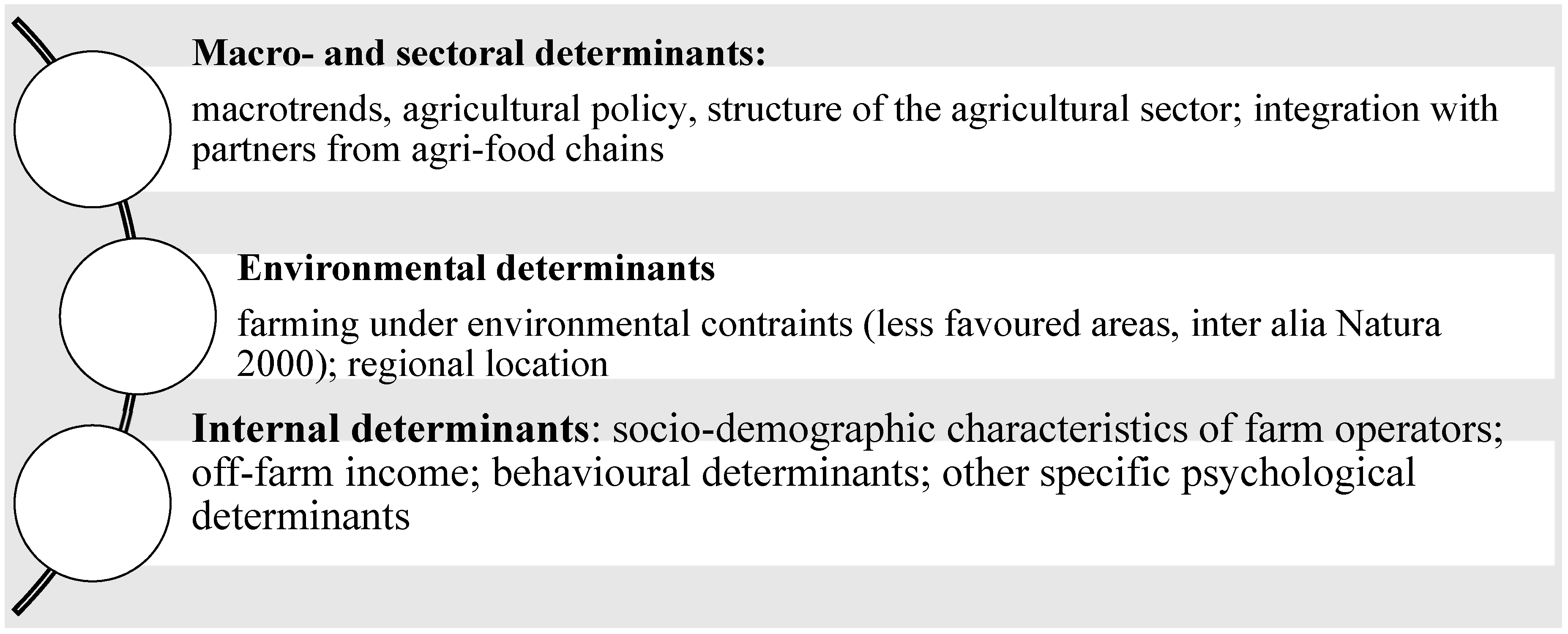
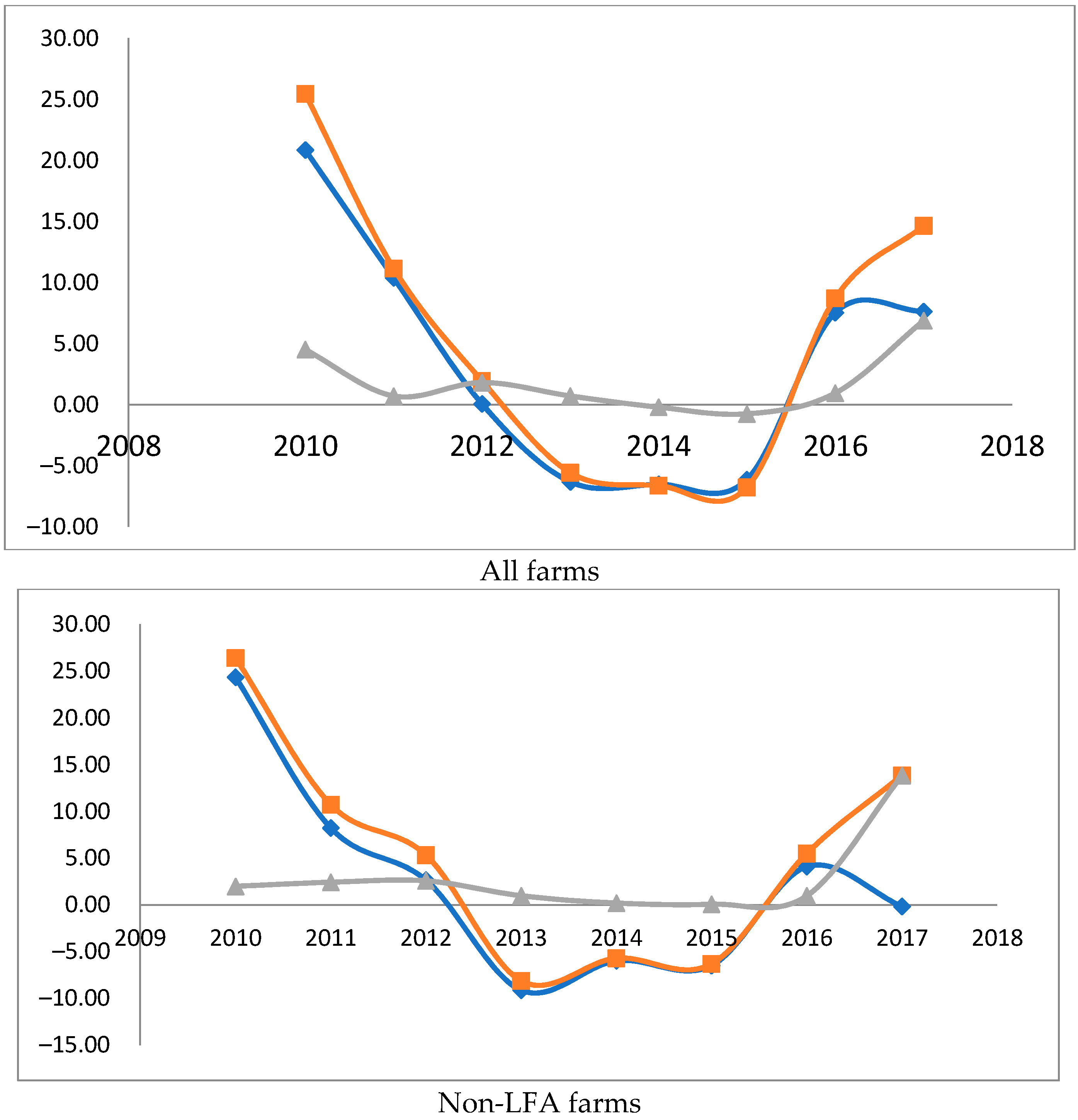
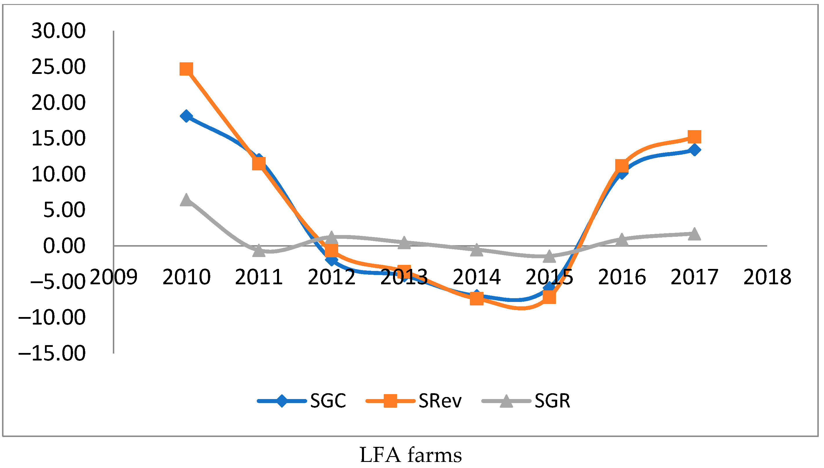
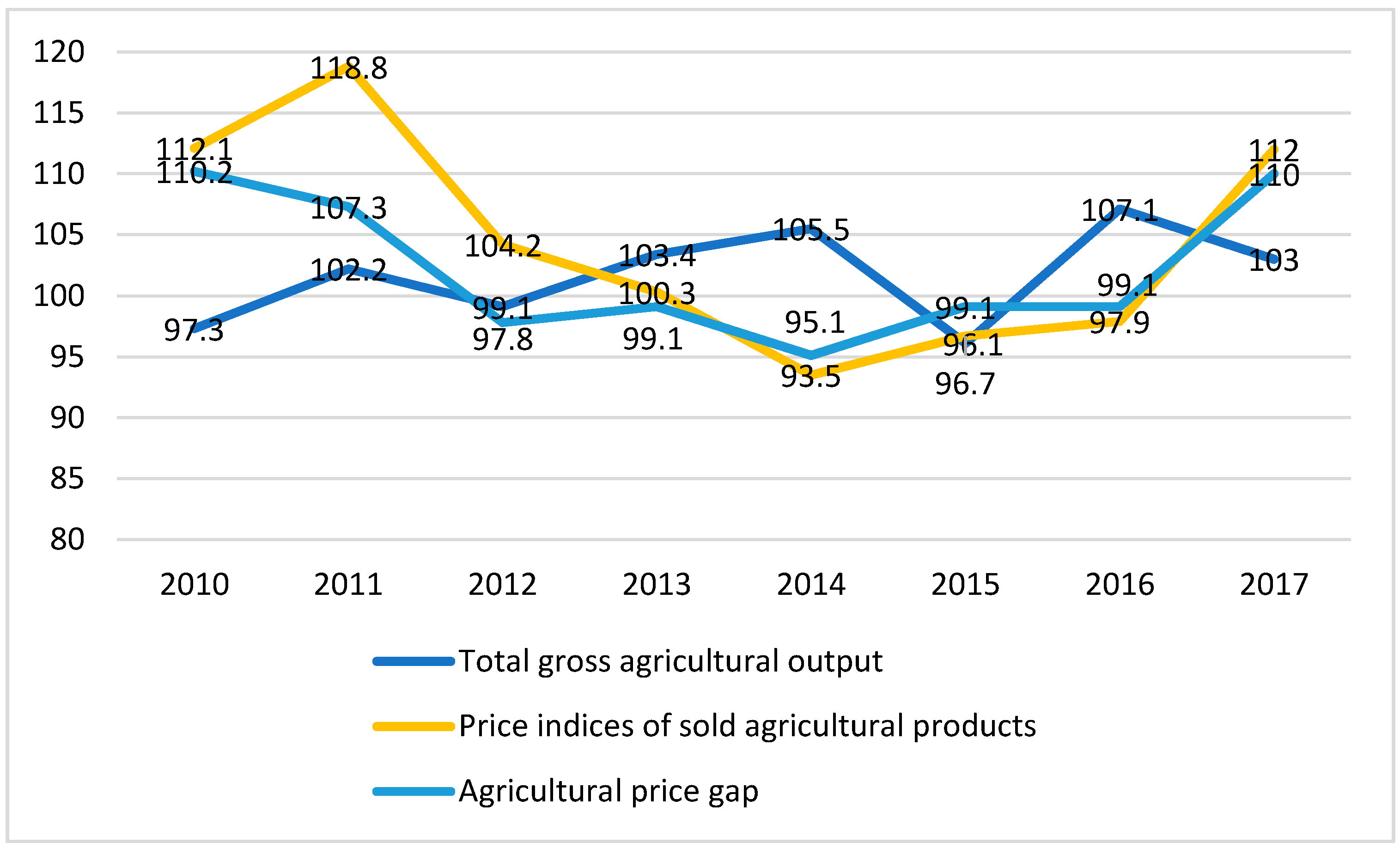


