Abstract
Landslides and collapses are common geological hazards in mountainous areas, posing significant threats to the lives and property of residents. Therefore, early identification of disasters is of great significance for disaster prevention. In this study, we used Small Baseline Subset Interferometric Synthetic Aperture Radar (SBAS-InSAR) technology to process C-band Sentinel-1A images to monitor the surface deformation from Songpinggou to Feihong in Maoxian County, Sichuan Province. Visibility analysis was used to remove the influence of geometric distortion on the SAR images and retain deformation information in the visible area. Hot spot and kernel density analyses were performed on the deformation data, and 18 deformation clusters were obtained. Velocity and slope data were integrated, and 26 disaster areas were interpreted from the 18 deformation clusters, including 20 potential landslides and 6 potential collapses. A detailed field investigation indicated that potential landslides No. 6 and No. 8 had developed cracks and were severely damaged, with a high probability of occurrence. Potential collapse No. 22 had developed fissures, exposing a dangerous rock mass and posing significant threats to the lives and property of residents. This study shows that the proposed method that combines visibility analysis, InSAR deformation rates, and spatial analysis can quickly and accurately identify potential geological disasters and provide guidance for local disaster prevention and mitigation.
1. Introduction
Geological hazards are catastrophic events caused by natural or man-made factors [1,2] and include collapses, landslides, debris flows, karst surface collapses, ground fissures, and subsidence [3,4]. They typically occur in mountainous areas and are characterized by a sudden occurrence, accompanied by casualties, property losses, and environmental destruction [5,6,7]. For example, the Xinmo landslide on 24 June 2017 caused 83 casualties [8], and the Baige landslide on 10 October 2018 caused economic losses of approximately 6.8 billion yuan [9]. Therefore, the early identification of geological disasters is of great significance for disaster prevention and mitigation.
The identification of geological hazards is complex [10]. It is generally considered that surface deformation is an important indicator of potential geological disasters. In the past, experts analyzed macro-physiological features using field surveys to identify potential disasters such as landslides [11,12]. Traditional measurement methods, such as leveling measurements, global positioning systems (GPS), and global navigation satellite systems (GNSS), with a monitoring accuracy of centimeter-to-millimeter, have also been used to monitor surface deformation [13,14,15]. These methods are performed on a point-to-point basis. Therefore, for a large research area, the acquisition of monitoring data is relatively time-consuming and laborious [16,17], and in underdeveloped areas, the high cost limits their applications [18]. Moreover, the low spatial coverage of data is also a major challenge for researching geological hazards of the entire study area [19]. Due the generation of various high-precision, large-scale satellite Synthetic Aperture Radar (SAR) images [20], Interferometric Synthetic Aperture Radar (InSAR) technology has been increasingly used in recent years for surface deformation monitoring.
InSAR technology has the advantages of a large coverage area, high precision, and all-weather applications. Differential Interferometric Synthetic Aperture Radar (D-InSAR) technology was first used for ground deformation monitoring in 1989 and exhibited high monitoring accuracy [21,22]. Subsequently, the method was increasingly used for the surface deformation monitoring of geological disaster areas [23,24,25]. However, with the continuous improvement of InSAR technology, experts found that D-InSAR is susceptible to external factors and has decorrelation problems, limiting its monitoring accuracy. Therefore, time-series InSAR technologies, such as Persistent Scatterer Interferometric SAR (PS-InSAR) and Small Baseline Subset (SBAS)-InSAR, were proposed by Ferretti et al. [26] and Berardino et.al. [27] in 2000 and 2002, respectively. PS-InSAR was used for urban surface deformation monitoring [28,29,30], whereas SBAS-InSAR is applicable to urban and non-urban areas [31,32,33,34]. Therefore, SBAS-InSAR technology has been widely used in research on geological disasters.
The SBAS-InSAR technology uses a singular value decomposition (SVD) algorithm to perform time-series analysis on SAR images [27] and obtain the average annual deformation rate of the study area. Monitoring data obtained by SBAS-InSAR technology have the characteristics of many data points, wide distribution and high spatial correlation. In order to quickly and accurately identify abnormal deformation regions, some studies used hot spot analysis to process the results of monitoring. Hot spot analysis is a viable method for semi-automatic ground movements extraction [35]. By means of spatial statistics, the aggregation degree of deformation points is calculated. Then, high-low clustering is divided according to the standard normal distribution to highlight the regions with fast motion [36,37,38,39]. Moreover, kernel density analysis is also an effective spatial statistical method, which calculates the density around each point by constructing a smooth surface and realizes the transformation from discrete objects to continuous fields, and then visualizes the abnormal area to make it more prominent [40]. For these abnormal deformation areas, the reliability of the results can be verified by numerical simulation, comparison of GPS monitoring results, or field investigations of the abnormal area [18,41,42]. Numerous studies have shown that SBAS-InSAR technology has high monitoring accuracy [43], providing excellent results for the identification of landslides and other geological disasters [44,45,46]. However, most studies have ignored the geometric distortions of the satellite images, including shadows, layover, and foreshortening [45], which are especially pronounced in mountainous areas. These phenomena degrade the quality of the SAR images and result in invalid deformation data. Therefore, how to obtain effective monitoring data and identify geological disasters is of great significance.
In order to obtain reliable deformation information and quickly and effectively identify potential geological hazards in Maoxian County, we combined the terrain information of Maoxian County with the satellite parameters of Sentinel-1A ascending data to conduct a visibility analysis. The study area is divided into visible and invisible areas to eliminate the influence of image geometric distortion on monitoring data. Then, the SBAS-InSAR deformation rate in the visible area is extracted, and hot spot analysis is performed to obtain the fast-moving area. In order to highlight the abnormal deformation areas, based on the result of the hot spot analysis, we performed kernel density analysis. Deformation rate, the structural characteristics of the slope, and information from Google images are used to identify different types of potential geological hazards in these abnormal areas. Finally, field investigations are used to verify the types of potential geological disasters and their probability of occurrence.
2. Study Area
The study area is located in Mao County, Sichuan Province, Southwest China (Figure 1), extending from Songpinggou to Feihong, with a total area of 611.8 km2. The geographic coordinates of the study area are between 103°32′~103°47′ E and 31°47′~32°9′ N. The area is located on the upper Minjiang River, in the transition zone from the Qinghai-Tibet Plateau to the Sichuan Basin. The geomorphology is dominated by alpine valleys, with Minshan Mountain in the north, Longmen Mountain in the south, and Qionglai Mountain in the west. The terrain is steep, sloping from northwest to southeast, with a relative elevation difference of 1000~2500 m in the northwest and 500~1500 m in the southeast.
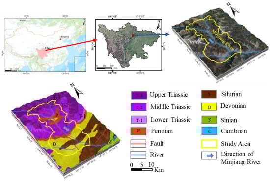
Figure 1.
Location, topography, and geology map of the study area.
The region is characterized by a complex geological structure and strong neotectonic movements and seismic activities. The peak seismic acceleration is 0.20 g, making the area prone to geological hazards such as landslides and debris flows. The Minjiang fault, Songpinggou fault, and Shidaguan fault are the main fault structures in the study area, causing lithological fractures and inversions. The main exposed strata in the research area are Triassic, Permian, Devonian, and Silurian. The lithology of the research area consists of the upper Triassic series (T3x, T3zh) metamorphic sandstone and sericite slate, the middle Triassic series (T2z) metamorphic sandstone and slate, the lower Triassic series (T1b) phyllite and slate, Permian siliceous intercalated with carbonatite, Devonian gray-black metamorphic sandstone and phyllite, and Silurian green sericite slate and quartz sandstone.
The area has a plateau monsoon climate, and vertical differences in the climate and regional differences are pronounced due to large elevation differences, resulting in a complex local climate. The average annual temperature is 11 °C, and the minimum and maximum temperatures are −11.6 °C and 32.2 °C, respectively. The rainy season lasts from May to October, with a maximum daily rainfall of 75.2 mm, average annual rainfall of about 480 mm, maximum annual rainfall of 560 mm, and minimum annual rainfall of 335.5 mm. The area is prone to rainstorms, floods, and debris flows [47].
3. Data and Methodology
3.1. Data
A total of 38 Sentinel-1A satellite images (ascending data) acquired from 14 October 2014 to 13 August 2019 were obtained and processed using SBAS- InSAR technology to calculate the deformation rate. The wavelength is 5.6 cm in the C-band. Sentinel-1A is a high-resolution SAR satellite launched by the European Space Agency in April 2014. It has an orbital altitude of 693 km and an inclination of 98.18°. The satellite revisit time is 12 days for a single satellite and 6 days for the two-satellite constellation [48]. The sensor has four imaging modes and polarization methods. In this study, we selected the interferometric wide swath (IW) slant-distance single look complex (SLC) mode, with a width of 250 km and a spatial resolution of 5 × 20 m (Figure 2); the relative orbit number is T128 (in Table 1).
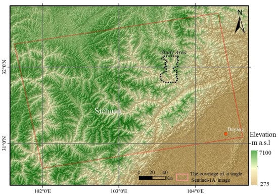
Figure 2.
The coverage of a single Sentinel-1A SAR image.

Table 1.
Basic information on the Sentinel-1A images.
Precision orbit files were generated 21 days after GNSS data were obtained, and accuracy exceeded 5 cm. Two types of Shuttle Radar Topography Mission Digital Elevation Model (STRM DEM) products are available: the 1 arc-second product with a resolution of 30 m and the 3 arc-second product with a resolution of 90 m [49]. The former was used in conjunction with the SBAS-InSAR for terrain phase removal and visibility analysis [18].
3.2. Methodology
3.2.1. Time Series InSAR Analysis with SBAS
SBAS-InSAR is a time-series InSAR technology based on D-InSAR that overcomes the problems of spatiotemporal decorrelation and atmospheric interference [49]. The SBAS-InSAR technology was proposed by Berandino et al. in 2002 [27]. It is a time-series method based on multi-master images used to obtain the deformation rate of the study area using the SVD method of a matrix.
Assuming that N + 1 SAR images were acquired for the same region at regular times (t0, …, tN), M differential interferograms can be generated. The inequality of M is defined as follows:
For the differential interferogram j generated from the images acquired at and (), the phase of any point is as follows:
where and are the phase of two images at the point ; is the phase formed by the cumulative deformation of the line of sight (LOS) at and relative to ; and the phase errors caused by topography, orbit, atmosphere, and noise are represented by [50,51].
The Environment for Visualizing Images (ENVI) software and its subordinate module SARscape were employed to process SAR images from the research area. Six steps were used: generation of the connection graph, interferometric processing, refinement and re-flattening, first inversion, second inversion, and geocoding. The processing flowchart is shown in Figure 3.
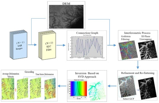
Figure 3.
Flowchart of SBAS-InSAR processing. Note: GCP—ground control points.
According to the geological conditions of the study area, the spatial baseline and temporal baseline were set at 2% and 180 d, respectively. After three-dimensional (3D) unwrapping, 109 interferometric pairs were generated with a maximum spatial baseline of 116.3 m and a minimum of 59 m. As shown in Figure 4, the 14 February 2019 image (yellow point) was selected by the software as the super master image. Then, the Goldstein filter and 3D unwrapping method were used for interferometric processing, and the unwrapping threshold was set to 0.2. After that, 12 interferometric pairs with poor coherence were deleted, and 97 interferometric pairs were used in subsequent time-series analysis. In the non-deformation region, an appropriate amount of ground control points was uniformly selected for refinement and re-flattening, and the control points were screened to ensure that there were sufficient control points and deviation was within 2.5. In the first inversion, we selected the linear model to estimate the surface deformation rate and residual topography. Ground control points were introduced in the second inversion to eliminate atmospheric phase interference and obtain a more accurate time-series displacement. Finally, geocoding was performed to obtain the average deformation velocity and displacement of the study area in the direction of the radar LOS.
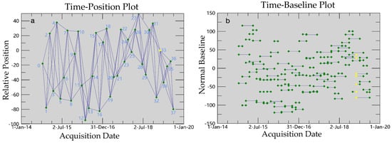
Figure 4.
The time-position plot (a) and the time–baseline plot (b).
3.2.2. Visibility Analysis
SAR data are affected by the azimuth and incident angle of the satellite, resulting in foreshortening, layover and shadow of the image [52]. In mountainous areas, if the incident angle is greater than the slope angle, foreshortening occurs on the slope facing towards the antenna, causing the target to be compressed on the SAR image. While the incident angle is less than the slope angle, the signal of the radar will reach the top of the slope first, which induces the layover and causes the top and bottom of the slope to be inverted. The shadow phenomenon occurs on a slope facing away from the satellite, of which the slope angle is greater than the incident angle of the satellite [45]. The signal of the radar cannot reach the slope, causing a black area on the image. These phenomena form the invisible area of the satellite, which reduces the quality of the SAR image and cannot provide effective deformation information, adversely affecting the monitoring accuracy. Therefore, we used ArcGIS software and the Digital Elevation Model (DEM) of the study area to determine the slope and aspect and integrated the incident angle of the satellite’s ascending orbit to perform reclassification with raster calculator tools to obtain the terrain-based visibility map of the Sentinel-1A data. The processing flowchart is shown in Figure 5.
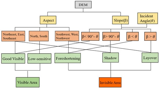
Figure 5.
Flowchart of the visibility analysis of the study area. Note—θ is the average incident angle of the Sentinel-1A images in Table 1.
According to the result of the aspect analysis, the angles 0°–22.5°, 337.50°–360°, and 157.5°–202.5° were divided into north and south aspects; 22.5°–157.5° were divided into northeast, east, and southeast aspects; and 202.5°–337.5° were divided into southwest, west, and northwest aspects. Since Sentinel-1A operates in a near-polar mode, the radar LOS is less sensitive to north-south deformation; thus, the north-south direction was divided into a low sensitive area. As shown in Figure 5, the research area was classified into five groups: good visible, low sensitive, shadow, foreshortening, and layover [45]. Finally, the good visible area and low sensitive area were combined into the visible area, and the shadow, foreshortening, and layover areas were classified as the invisible area.
3.2.3. Spatial Statistical Analysis
Hot spot analysis and kernel density analysis were performed using the spatial statistical analysis tool in ArcGIS software to identify the areas with a rapid deformation rate.
Hot Spot Analysis
Hot spot analysis was proposed to calculate the degree of aggregation of the deformation points [39]. For a detection location, i, within a given range of distance, the ratio of the sum of the attribute values of the features at adjacent locations to the sum of the attribute values of the features at all locations is used to calculate whether i and the surrounding adjacent location features are high-value aggregations or low-value aggregations. The equation is as follows:
where represents the spatial weight matrix of the topological relationship between the elements i and j; represents the sum of the attribute values of all elements within the distance d of the point (excluding ); and is the comprehensive attribute value of all elements (not including ).
After hot spot analysis, we could obtain the G_Bin and Z-score of each element. Here, G_Bin indicated the confidence interval, which was used to obtain statistically significant points. Z-score is expressed as a multiple of the standard deviation and was used for kernel density analysis.
Kernel Density Analysis
Kernel density analysis was used to calculate the density of the elements in a neighborhood around the elements to determine the degree of aggregation of the point elements or polyline elements in each grid cell. In analysis of the point elements, it is assumed that a smooth, curved surface is fitted over each point. The surface value is highest at the position of the point and gradually decreases with an increase in the distance to the point. The volume of the space enclosed by the surface and the plane below is equal to the value of the population field of this point. If the value of the population field is specified as NONE, the volume is 1. The density of each output raster cell is the sum of the values of all core surfaces superimposed on the center of the raster cell.
The functional equation of the kernel density analysis is as follows:
where is the probability density function; is the window size; is the number of deformation points; and is the kernel function.
4. Results and Discussion
4.1. Ground Deformation and Spatial Distribution
According to the processing in Section 3.2, the average deformation rate of the LOS in the area from 2014 to 2019, the visibility analysis map, and spatial analysis results were obtained.
As shown in the velocity map in Figure 6a, negative values indicate that the deformation motion is away from the satellite, and positive values represent the uplift of the ground and the motion toward the satellite. The deformation velocity of the study area ranges from −46.50 mm/y to 39.87 mm/y, and the average rate is −6.24 mm/y. Most values are concentrated in the range of −10 mm/y–10 mm/y, which indicates that the deformation of the study area is relatively stable [45]. A total of 410,047 coherence points were obtained; 120,552 points had a rate greater than 0, and 289,493 points had a rate less than 0. The southern part of the study area had 5 obvious deformation zones, as shown in the orange circles in Figure 6a, with a velocity of less than −35 mm/y. Results of the visibility analysis of the Sentinel-1A ascending data are shown in Figure 6b. The area was divided into visible areas and invisible areas. The visible area (green) covers 377.7 km2, accounting for about 61.7%; it includes the good visible area (214.8 km2) and the low sensitive area (162.9 km2). The invisible area covers 234.1 km2, accounting for 38.3% of the total and consists of the foreshortening area (blue) (162.9 km2), layover area (yellow) (70.6 km2), and shadow area (red) (0.6 km2). The invisible areas are located primarily on southwest-facing slopes. Therefore, most of the deformation information was obtained on northeast-facing slopes. The result of the terrain visibility analysis shows that Sentinel-1A ascending data are well suited for ground deformation monitoring in the study area.
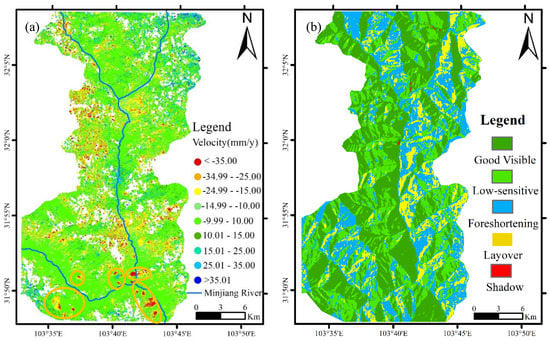
Figure 6.
(a) Annual average ground deformation rate in the study area. (b) Visibility map of the study area. Note: the orange circle represents the area with an abnormal deformation rate.
To ensure the accuracy of the monitoring result, we deleted 118,324 deformation points in the invisible area and retained the points in the visible area, as shown in Figure 7a, for a total of 291,723 deformation points. Hot spot analysis showed that 84.3% of the deformation points had significant spatial aggregation, 3.6% of the points had a certain degree of aggregation, and 1.8% of the deformation points might be a random distribution. In addition, 30,078 points had a value of 0, indicating that these points were randomly distributed, were not statistically significant, and should be eliminated. Therefore, 89.7% of the deformation points were statistically significant and used for kernel density analysis. The result of the kernel density analysis is shown in Figure 7b. Red represents low-value aggregation, and green represents high-value aggregation. Similar to the velocity results in Figure 7a, red represents aggregation where the rate is less than 0. As shown in Figure 7b, 18 deformation clusters were obtained. Most were located on both sides of the river, and some were located in the valley. Google Earth images and the deformation rate and slope were used to interpret the 18 regions in Figure 7b; 26 potential geological hazards were identified in these regions.
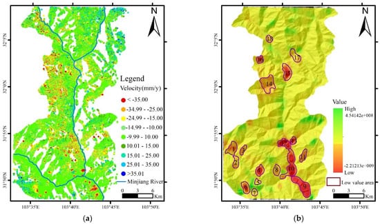
Figure 7.
(a) The annual average ground deformation rate of the visible area and the result of kernel density analysis (b). Note: numbers 1 to 18 in the figure represent areas where rates are conspicuously gathered.
An area was classified as a landslide according to the morphology of the slope, the presence of cracks, or other signs of failure [53,54]. If there were no coherence points in a certain area on the slope and the deformation points around it existed, and a rock mass or gravel was visible in the images, the area was classified as a collapse. According to this classification standard, the primary geological disaster types in the study area were landslides and collapses. As shown in Table 2, we observed 20 potential landslides and 6 potential collapses on both sides of the Minjiang River.
Table 2.
Classification of the geological hazards.
4.2. Discussion
In this work, two types of potential geological hazards (landslides and collapses) were identified in the study area, and the hazard areas were numbered from 1 to 26. A detailed analysis was conducted by integrating the slope deformation rate and field survey results.
4.2.1. Landslides
The potential landslide area 8 was used as an example. This landslide is located on the left bank of the Minjiang River, with geographical coordinates of 103°43′14.66″ E and 31°49′39.35″ N. The slope is steep, and the relative relief is 1157 m. The velocity map of the landslide is shown in Figure 8a. The deformation velocity of the landslide is between −46.5 mm/y and 39.87 mm/y. There is a lack of coherence points at the top and bottom of the slope, which is attributed to the large deformation of the rock and soil at the top and manual excavation at the bottom [55,56]. The deformation rate in the middle of the slope is substantially higher than that on both sides and is the main deformation zone. Therefore, field investigations were conducted in this area.
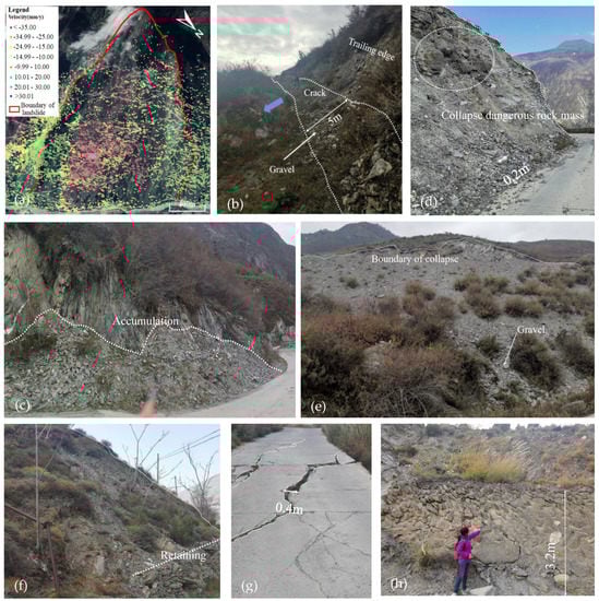
Figure 8.
Field photos of potential landslide 8. (a) Velocity map of the landslide. (b) Crack at the trailing edge. (c) Accumulation area of the rock and soil. (d,e) A small-scale collapse. (f) A small-scale landslide. (g) Cracks in the road. (h) Cracked retaining wall. Note: the red curve in (a) represents the boundary of the landslide, and the blue arrow in (b) represents the direction of slipping.
It was found that the slope exhibited local deformation, and cracks were well developed and widely distributed; many small-scale collapses and landslides were observed. The survey point in Figure 8b is located at the top of the slope. The landslide occurred due to the influence of rainfall and earthquakes [57], and the trailing edge was exposed, resulting in a large tensile crack with a width of about 5 m. A lot of gravel was observed, and the dominant particle size was about 20 cm. The field investigation showed that the sliding distance was about 40 m. The downward sliding of the rock and soil destroyed the road and guardrails, formed cracks, caused economic losses, and threatened traffic safety [58]. The rock, soil, and gravel that slid down the slope were mostly accumulated on the inside of the road in a fan shape, as shown in Figure 8c. The top of the accumulated material was gravel, particles were mostly smaller than 0.2 m, and the bottom consisted of soil or gravel with smaller particles.
Figure 8d,e show two small-scale collapses, with heights of about 10 m. The surface and the bottom of the slope was covered by gravel due to the failure of the rock mass, and the particle size was mostly less than 0.2 m. The road below the slope was affected by the collapse, exhibiting cracks with widths of 2–6 cm and tens of meters in length. In Figure 8e, a dangerous rock mass is observed at the height of about 6 m. This relatively large area may collapse due to rainfall and other factors, causing potential harm. During the investigation, many small-scale landslides were observed; Figure 8f shows a small landslide at the bottom of the slope. Part of the retaining wall was destroyed due to sliding rock and soil. In addition, the landslide caused serious damage to the road and formed tension cracks. As shown in Figure 8g, the cracks extended along the road with a length of about 35 m and a width of up to 0.4 m. The same phenomenon occurred at the toe of the slope, as shown in Figure 8h. The photo shows a retaining wall with a height of about 3.2 m. The retaining wall was pushed forward by the force of the downward movement of the upper accumulation layer and the downward collapse of boulders. The retaining wall had many penetrating cracks. If the accumulated layer continues to move downward, the retaining wall will likely collapse.
The field investigation showed substantial small-scale damage, although the slope was relatively stable, and the observations were consistent with the results of the SBAS-InSAR analysis. The slope was affected by natural factors and engineering activities. When the local damage is severe, widespread damage may occur. At this time, a landslide is highly likely, posing a significant threat to the lives and property of local residents.
4.2.2. Collapse
The potential collapse in area 22 is used as an example of the analysis.
The potential collapse is located on the right bank of the Minjiang River, with geographic coordinates of 103°40′40.884″ E, 32°01′11.113″ N, and a slope of about 40°. The height of the slope is about 175 m, and the elevations at the front and rear edges are 2032 m and 2207 m, respectively. As shown in Figure 9a, the coherence points are concentrated in the middle of the slope. The maximum deformation rate of the slope is −43.94 mm/y, and the deformation point is seriously missing [59]. The Google earth image shows that the rock and soil mass at the trailing edge is exposed, which is attributed to the collapse of the upper dangerous rock mass.
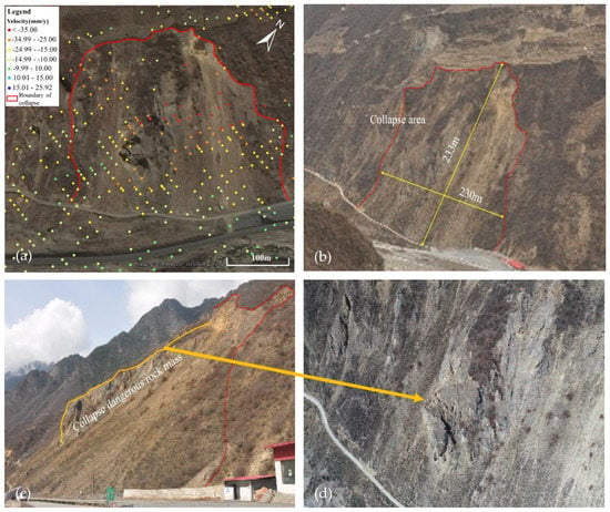
Figure 9.
(a) Velocity map of the collapse. (b–d) Field photos of the potential collapse. (b) The range of the collapse. (c,d) A dangerous rock mass on the slope. Note—the red dotted line represents the boundary of the collapse, and the orange circle represents the dangerous rock mass.
The field investigation indicated that the slope was about 233 m in length and 230 m in width (Figure 9b) with an area of about 53,600 m2 and a volume of about 100,000 m3. The area is a medium-sized sliding collapse [60]. The slope consists of three parts: the lower slope covered by soil, the middle slope consisting of broken bedrock, and the upper slope, which is a cliff. The slope of the steep cliff is between 30° and 40°, and the area extends along the right bank of the Minjiang River, with exposed bedrock exhibiting strong weathering and erosion. The lithology is metamorphic sandstone with slate, and the attitude of the rock formation is 187°/63° (dip angle). The middle part of the slope is the collapsed dangerous rock mass, which is broken and has developed tension cracks with a width of about 5–10 cm. The collapsed body is steep, with an angle of about 60°, and it protrudes from the slope as shown in Figure 9c,d. The material of the lower slope is mainly rubble intercalated with clay sand with a high argillaceous content. The rubble has different particle sizes, and the larger ones have diameters of several meters. Due to the development of slope cracks, the rock mass is divided into multiple blocks, forming many dangerous rock masses. The largest block is 5 m × 4 m × 3 m. The collapsed area will increase in depth due to rainfall and earthquakes, resulting in a collapse disaster. Therefore, the slope has a high probability of collapse. Since the slope is near a highway with a restaurant beside the road, the safety of people and property will be threatened if a collapse occurs [61].
5. Conclusions
In this research, we proposed SBAS-InSAR technology for processing 38 Sentinel-1A ascending SAR images for monitoring ground deformation from Songpinggou to Feihong in Mao County. Reliable deformation information was obtained from visibility analysis of the study area, improving the accuracy of the monitoring results. The analysis of the reliable deformation data combined with interpretation of Google Earth images quickly provided information on deformation areas, facilitating the identification of potential geological disaster areas. The results were verified by field surveys. The main conclusions are as follows:
The average deformation rate from 14 October 2014 to 13 August 2019 was between −46.50 mm/y and 39.87 mm/y. Most of the deformation rates of the 410,047 deformation points fell in the range of −10 to 10 mm/y. The entire study area was relatively stable, but deformation areas were observed on both sides of the Minjiang River.
Visibility analysis indicated that the visible area occupied about 61.7% of the study area, with 291,723 reliable deformation points. Invisible areas were mostly located on southwest-facing slopes, accounted for 38.3% of the total area and included 118,324 unreliable deformation points. The results showed that Sentinel-1A ascending data were highly suitable for ground deformation monitoring in this area.
Spatial statistical analysis provided 18 deformation clusters, and 26 potential disaster areas were interpreted with the help of Google Earth images and deformation rate data. Potential landslides were the dominant type of geological disaster in Mao County, accounting for 76.9% of all disasters, whereas potential collapses accounted for 23.1%.
The field investigation showed that the occurrence probability of potential landslides at the No. 6 and No. 8 areas was relatively high due to failure characteristics and cracks. The No. 22 potential collapse also exhibited a high probability of occurrence, posing threats to the lives and property of residents.
Although the method used in this paper can effectively identify geological hazards, it can only be used as a preliminary method for disaster identification. In the next step, it is necessary to use various methods such as the field investigation, Unmanned Aerial Vehicle (UAV), LiDAR and GNSS to conduct more detailed surface deformation analysis of the landslide, and borehole inclinometers should be installed at different depths to accurately monitor the deep deformation of the landslide and estimate the date of the hazard. In addition, in order to obtain effective deformation points, we deleted points in invisible areas. However, this does not mean that there are no geological disasters in these areas. According the previous research, more accurate and extensive monitoring data can be obtained through SAR data of different band, resolution, and orbital directions and sensors to realize disaster identification in invisible areas.
In general, this work proposed an effective preliminary method for monitoring ground deformation in mountainous areas and the rapid identification of geological disasters from Songpinggou to Feihong in Mao County. The approach provides a basis for disaster prevention and mitigation planning by the government.
Author Contributions
Conceptualization, C.C. and K.Z.; methodology, C.C., K.Z., P.X. and X.D.; software, K.Z. and Y.L.; validation, L.Z.; formal analysis, C.C. and K.Z.; investigation, Y.L.; resources, K.Z.; data curation, C.C. and K.Z.; writing—original draft preparation, K.Z.; writing—review & editing, C.C.; visualization, K.Z.; supervision, C.C.; project administration, P.X.; funding acquisition, P.X. All authors have read and agreed to the published version of the manuscript.
Funding
This work was financially supported by the National Key Research and Development Program of China (No. 2017YFC1501004), the National Nature Science Foundation of China (No. 41807227).
Institutional Review Board Statement
Not applicable.
Informed Consent Statement
Not applicable.
Data Availability Statement
The data presented in this study are available on request from the corresponding author. The data are not publicly available due to privacy.
Conflicts of Interest
The authors declare no conflict of interest.
References
- Tan, Q.; Huang, Y.; Hu, J.; Zhou, P.; Hu, J. Application of artificial neural network model based on GIS in geological hazard zoning. Neural Comput. Appl. 2020. [Google Scholar] [CrossRef]
- Zhang, X.; Wu, Y.; Zhai, E.; Ye, P. Coupling analysis of the heat-water dynamics and frozen depth in a seasonally frozen zone. J. Hydrol. 2020. [Google Scholar] [CrossRef]
- Huang, P.; Peng, L.; Pan, H. Linking the Random Forests Model and GIS to Assess Geo-Hazards Risk: A Case Study in Shifang County, China. IEEE Access 2020, 8, 28033–28042. [Google Scholar] [CrossRef]
- Yingran, L.; Hailing, S.; Jian, G. Geologic hazard susceptibility and disaster risk mapping based on information value model for the MianChi county, China. IOP Conf. Ser. Earth Environ. Sci. 2018, 199. [Google Scholar] [CrossRef]
- Ding, W.; Tang, J.; Tian, X.; Liu, X.; Li, D.; Geng, Y. Distribution Characteristics of Geo-hazards in a Reservoir Area, South Gansu Province, China. Indian J. Geo-Mar. Sci. 2020, 49, 233–240. [Google Scholar]
- Wu, S.-N.; Lei, Y.; Cui, P.; Chen, R.; Yin, P.-H. Chinese public participation monitoring and warning system for geological hazards. J. Mt. Sci. 2020, 17, 1553–1564. [Google Scholar] [CrossRef]
- Shi, X.; Yang, C.; Zhang, L.; Jiang, H.; Liao, M.; Zhang, L.; Liu, X. Mapping and characterizing displacements of active loess slopes along the upstream Yellow River with multi-temporal InSAR datasets. Sci. Total Environ. 2019, 674, 200–210. [Google Scholar] [CrossRef]
- Yang, L.; Wang, W.; Zhang, N.; Wei, Y. Characteristics and numerical runout modeling analysis of the Xinmo landslide in Sichuan, China. Earth Sci. Res. J. 2020, 24, 169–181. [Google Scholar] [CrossRef]
- Tian, S.F.; Chen, N.S.; Wu, H.; Yang, C.Y.; Zhong, Z.; Rahman, M. New insights into the occurrence of the Baige landslide along the Jinsha River in Tibet. Landslides 2020, 17, 1207–1216. [Google Scholar] [CrossRef]
- Liu, Y.; Wu, L. Geological Disaster Recognition on Optical Remote Sensing Images Using Deep Learning. Procedia Comput. Sci. 2016, 91, 566–575. [Google Scholar] [CrossRef]
- Rogers, J.D.; Chung, J.-W. Applying Terzaghi’s method of slope characterization to the recognition of Holocene land slippage. Geomorphology 2016, 265, 24–44. [Google Scholar] [CrossRef]
- Wang, H.; Nie, D.; Tuo, X.; Zhong, Y. Research on crack monitoring at the trailing edge of landslides based on image processing. Landslides 2020, 17, 985–1007. [Google Scholar] [CrossRef]
- Bianchini Ciampoli, L.; Gagliardi, V.; Ferrante, C.; Calvi, A.; D’Amico, F.; Tosti, F. Displacement Monitoring in Airport Runways by Persistent Scatterers SAR Interferometry. Remote Sens. 2020, 12, 3564. [Google Scholar] [CrossRef]
- Zhao, C.; Kang, Y.; Zhang, Q.; Lu, Z.; Li, B. Landslide Identification and Monitoring along the Jinsha River Catchment (Wudongde Reservoir Area), China, Using the InSAR Method. Remote Sens. 2018, 10, 993. [Google Scholar] [CrossRef]
- Shahzad, N.; Ding, X.; Wu, S.; Liang, H. Ground Deformation and Its Causes in Abbottabad City, Pakistan from Sentinel-1A Data and MT-InSAR. Remote Sens. 2020, 12, 3442. [Google Scholar] [CrossRef]
- Fan, H.; Lu, L.; Yao, Y. Method Combining Probability Integration Model and a Small Baseline Subset for Time Series Monitoring of Mining Subsidence. Remote Sens. 2018, 10, 1444. [Google Scholar] [CrossRef]
- Jung, H.C.; Kim, S.-W.; Jung, H.-S.; Min, K.D.; Won, J.-S. Satellite observation of coal mining subsidence by persistent scatterer analysis. Eng. Geol. 2007, 92, 1–13. [Google Scholar] [CrossRef]
- Zhou, C.; Cao, Y.; Yin, K.; Wang, Y.; Shi, X.; Catani, F.; Ahmed, B. Landslide Characterization Applying Sentinel-1 Images and InSAR Technique: The Muyubao Landslide in the Three Gorges Reservoir Area, China. Remote Sens. 2020, 12, 3385. [Google Scholar] [CrossRef]
- Zheng, M.; Deng, K.; Fan, H.; Du, S. Monitoring and Analysis of Surface Deformation in Mining Area Based on InSAR and GRACE. Remote Sens. 2018, 10, 1392. [Google Scholar] [CrossRef]
- Wang, Z.; Liu, J.; Wang, J.; Wang, L.; Luo, M.; Wang, Z.; Ni, P.; Li, H. Resolving and Analyzing Landfast Ice Deformation by InSAR Technology Combined with Sentinel-1A Ascending and Descending Orbits Data. Sensors 2020, 20, 6561. [Google Scholar] [CrossRef]
- Rizo, V.; Tesauro, M. SAR interferometry and field data of Randazzo landslide (Eastern Sicily, Italy). Phys. Chem. Earth Part B Hydrol. Ocean. Atmos. 2000, 25, 771–780. [Google Scholar] [CrossRef]
- Gabriel, A.K.; Goldstein, R.M.; Zebker, H.A. Mapping small elevation changes over large areas: Differential radar interferometry. J. Geophys. Res. 1989, 94. [Google Scholar] [CrossRef]
- Tesauro, M.; Berardino, P.; Lanari, R.; Sansosti, E.; Fornaro, G.; Franceschetti, G. Urban subsidence inside the city of Napoli (Italy) observed by satellite radar interferometry. Geophys. Res. Lett. 2000, 27, 1961–1964. [Google Scholar] [CrossRef]
- Zhang, L.; Lu, Z.; Ding, X.; Jung, H.-S.; Feng, G.; Lee, C.-W. Mapping ground surface deformation using temporarily coherent point SAR interferometry: Application to Los Angeles Basin. Remote Sens. Environ. 2012, 117, 429–439. [Google Scholar] [CrossRef]
- Zheng, W.; Hu, J.; Zhang, W.; Yang, C.; Li, Z.; Zhu, J. Potential of geosynchronous SAR interferometric measurements in estimating three-dimensional surface displacements. Sci. China Inf. Sci. 2017, 60. [Google Scholar] [CrossRef]
- Ferretti, A.; Prati, C.; Rocca, F. Nonlinear subsidence rate estimation using permanent scatterers in differential SAR interferometry. IEEE Trans. Geosci. Remote Sens. 2000, 38, 2202–2212. [Google Scholar] [CrossRef]
- Berardino, P.; Fornaro, G.; Lanari, R.; Sansosti, E. A new algorithm for surface deformation monitoring based on small baseline differential SAR interferograms. IEEE Trans. Geosci. Remote Sens. 2002, 40, 2375–2383. [Google Scholar] [CrossRef]
- Goorabi, A.; Maghsoudi, Y.; Perissin, D. Monitoring of the ground displacement in the Isfahan, Iran, metropolitan area using persistent scatterer interferometric synthetic aperture radar technique. J. Appl. Remote Sens. 2020, 14. [Google Scholar] [CrossRef]
- Yang, Q.; Ke, Y.; Zhang, D.; Chen, B.; Gong, H.; Lv, M.; Zhu, L.; Li, X. Multi-Scale Analysis of the Relationship between Land Subsidence and Buildings: A Case Study in an Eastern Beijing Urban Area Using the PS-InSAR Technique. Remote Sens. 2018, 10, 1006. [Google Scholar] [CrossRef]
- Wang, Z.; Balz, T.; Zhang, L.; Perissin, D.; Liao, M. Using TSX/TDX Pursuit Monostatic SAR Stacks for PS-InSAR Analysis in Urban Areas. Remote Sens. 2018, 11, 26. [Google Scholar] [CrossRef]
- Casu, F.; Lanari, R.; Sansosti, E.; Solaro, G.; Tizzani, P.; Poland, M.; Miklius, A. SBAS-InSAR analysis of surface deformation at Mauna Loa and Kilauea volcanoes in Hawaii. In Proceedings of the 2009 IEEE International Geoscience and Remote Sensing Symposium, Cape Town, South Africa, 12–17 July 2009; Volume 4. [Google Scholar]
- Liu, X.; Xing, X.; Wen, D.; Chen, L.; Yuan, Z.; Liu, B.; Tan, J. Mining-Induced Time-Series Deformation Investigation Based on SBAS-InSAR Technique: A Case Study of Drilling Water Solution Rock Salt Mine. Sensors 2019, 19, 5511. [Google Scholar] [CrossRef] [PubMed]
- Liu, L.; Yu, J.; Chen, B.; Wang, Y. Urban subsidence monitoring by SBAS-InSAR technique with multi-platform SAR images: A case study of Beijing Plain, China. Eur. J. Remote Sens. 2020, 1–13. [Google Scholar] [CrossRef]
- Wu, Q.; Jia, C.; Chen, S.; Li, H. SBAS-InSAR Based Deformation Detection of Urban Land, Created from Mega-Scale Mountain Excavating and Valley Filling in the Loess Plateau: The Case Study of Yan’an City. Remote Sens. 2019, 11, 1673. [Google Scholar] [CrossRef]
- Solari, L.; Del Soldato, M.; Montalti, R.; Bianchini, S.; Raspini, F.; Thuegaz, P.; Bertolo, D.; Tofani, V.; Casagli, N. A Sentinel-1 based hot-spot analysis: Landslide mapping in north-western Italy. Int. J. Remote Sens. 2019, 40, 7898–7921. [Google Scholar] [CrossRef]
- Mueller, C.; Micallef, A.; Spatola, D.; Wang, X. The Tsunami Inundation Hazard of the Maltese Islands (Central Mediterranean Sea): A Submarine Landslide and Earthquake Tsunami Scenario Study. Pure Appl. Geophys. 2019, 177, 1617–1638. [Google Scholar] [CrossRef]
- Solari, L.; Bianchini, S.; Franceschini, R.; Barra, A.; Monserrat, O.; Thuegaz, P.; Bertolo, D.; Crosetto, M.; Catani, F. Satellite interferometric data for landslide intensity evaluation in mountainous regions. Int. J. Appl. Earth Obs. Geoinf. 2020, 87. [Google Scholar] [CrossRef]
- Sultana, N.; Ricart Casadevall, S. Analysis of landslide-induced fatalities and injuries in Bangladesh: 2000–2018. Cogent Soc. Sci. 2020, 6. [Google Scholar] [CrossRef]
- Walter, M.; Mondal, P. A Rapidly Assessed Wetland Stress Index (RAWSI) Using Landsat 8 and Sentinel-1 Radar Data. Remote Sens. 2019, 11, 2549. [Google Scholar] [CrossRef]
- Calligaris, C.; Devoto, S.; Galve, J.; Zini, L.; Pérez-Peña, J. Integration of multi-criteria and nearest neighbour analysis with kernel density functions for improving sinkhole susceptibility models: The case study of Enemonzo (NE Italy). Int. J. Speleol. 2017, 46, 191–204. [Google Scholar] [CrossRef]
- Xu, Y.; George, D.L.; Kim, J.; Lu, Z.; Riley, M.; Griffin, T.; de la Fuente, J. Landslide monitoring and runout hazard assessment by integrating multi-source remote sensing and numerical models: An application to the Gold Basin landslide complex, northern Washington. Landslides 2020. [Google Scholar] [CrossRef]
- Tizzani, P.; Berardino, P.; Casu, F.; Euillades, P.; Manzo, M.; Ricciardi, G.P.; Zeni, G.; Lanari, R. Surface deformation of Long Valley Caldera and Mono Basin, California, investigated with the SBAS-InSAR approach. Remote Sens. Environ. 2007, 108, 277–289. [Google Scholar] [CrossRef]
- Zhao, F.; Meng, X.; Zhang, Y.; Chen, G.; Su, X.; Yue, D. Landslide Susceptibility Mapping of Karakorum Highway Combined with the Application of SBAS-InSAR Technology. Sensors 2019, 19, 2685. [Google Scholar] [CrossRef] [PubMed]
- Fustos, I.; Abarca-del-Rio, R.; Mardones, M.; Gonzalez, L.; Araya, L.R. Rainfall-induced landslide identification using numerical modelling: A southern Chile case. J. S. Am. Earth Sci. 2020, 101. [Google Scholar] [CrossRef]
- Guo, R.; Li, S.; Chen, Y.N.; Li, X.; Yuan, L. Identification and monitoring landslides in Longitudinal Range-Gorge Region with InSAR fusion integrated visibility analysis. Landslides 2020. [Google Scholar] [CrossRef]
- Zhang, M.; Ge, Y.; Xue, Y.; Zhao, J. Identification of geomorphological hazards in an underground coal mining area based on an improved region merging watershed algorithm. Arab. J. Geosci. 2020, 13. [Google Scholar] [CrossRef]
- Liu, W.; Cui, P.; Ge, Y.; Yi, Z. Paleosols identified by rock magnetic properties indicate dam-outburst events of the Min River, eastern Tibetan Plateau. Palaeogeogr. Palaeoclimatol. Palaeoecol. 2018, 508, 139–147. [Google Scholar] [CrossRef]
- Carlà, T.; Tofani, V.; Lombardi, L.; Raspini, F.; Bianchini, S.; Bertolo, D.; Thuegaz, P.; Casagli, N. Combination of GNSS, satellite InSAR, and GBInSAR remote sensing monitoring to improve the understanding of a large landslide in high alpine environment. Geomorphology 2019, 335, 62–75. [Google Scholar] [CrossRef]
- Du, W.; Ji, W.; Xu, L.; Wang, S. Deformation Time Series and Driving-Force Analysis of Glaciers in the Eastern Tienshan Mountains Using the SBAS InSAR Method. Int. J. Environ. Res. Public Health 2020, 17, 2836. [Google Scholar] [CrossRef]
- Yu, Q.; Wang, Q.; Yan, X.; Yang, T.; Song, S.; Yao, M.; Zhou, K.; Huang, X. Ground Deformation of the Chongming East Shoal Reclamation Area in Shanghai Based on SBAS-InSAR and Laboratory Tests. Remote Sens. 2020, 12, 1016. [Google Scholar] [CrossRef]
- Chen, D.; Chen, H.; Zhang, W.; Cao, C.; Zhu, K.; Yuan, X.; Du, Y. Characteristics of the Residual Surface Deformation of Multiple Abandoned Mined-Out Areas Based on a Field Investigation and SBAS-InSAR: A Case Study in Jilin, China. Remote Sens. 2020, 12, 3752. [Google Scholar] [CrossRef]
- Cigna, F.; Bianchini, S.; Casagli, N. How to assess landslide activity and intensity with Persistent Scatterer Interferometry (PSI): The PSI-based matrix approach. Landslides 2012, 10, 267–283. [Google Scholar] [CrossRef]
- Li, W.; Zhao, B.; Xu, Q.; Yang, F.; Fu, H.; Dai, C.; Wu, X. Deformation characteristics and failure mechanism of a reactivated landslide in Leidashi, Sichuan, China, on August 6, 2019: An emergency investigation report. Landslides 2020, 17, 1405–1413. [Google Scholar] [CrossRef]
- Dahal, R.K.; Hasegawa, S.; Nonomura, A.; Yamanaka, M.; Masuda, T.; Nishino, K. Failure characteristics of rainfall-induced shallow landslides in granitic terrains of Shikoku Island of Japan. Environ. Geol. 2008, 56, 1295–1310. [Google Scholar] [CrossRef]
- Nolesini, T.; Frodella, W.; Bianchini, S.; Casagli, N. Detecting Slope and Urban Potential Unstable Areas by Means of Multi-Platform Remote Sensing Techniques: The Volterra (Italy) Case Study. Remote Sens. 2016, 8, 746. [Google Scholar] [CrossRef]
- Crosetto, M.; Monserrat, O.; Cuevas-González, M.; Devanthéry, N.; Crippa, B. Persistent Scatterer Interferometry: A review. ISPRS J. Photogramm. Remote Sens. 2016, 115, 78–89. [Google Scholar] [CrossRef]
- Dille, A.; Kervyn, F.; Bibentyo, T.M.; Delvaux, D.; Ganza, G.B.; Mawe, G.I.; Buzera, C.K.; Nakito, E.S.; Moeyersons, J.; Monsieurs, E.; et al. Causes and triggers of deep-seated hillslope instability in the tropics—Insights from a 60-year record of Ikoma landslide (DR Congo). Geomorphology 2019, 345. [Google Scholar] [CrossRef]
- Fisseha, S.; Mewa, G. Road failure caused by landslide in north Ethiopia: A case study from Dedebit—Adi-Remets road segment. J. Afr. Earth Sci. 2016, 118, 65–74. [Google Scholar] [CrossRef]
- Pawluszek-Filipiak, K.; Borkowski, A. Integration of DInSAR and SBAS Techniques to Determine Mining-Related Deformations Using Sentinel-1 Data: The Case Study of Rydułtowy Mine in Poland. Remote Sens. 2020, 12, 242. [Google Scholar] [CrossRef]
- Simmons, J.; Elsworth, D.; Voight, B. Classification and idealized limit-equilibrium analyses of dome collapses at Soufrière Hills volcano, Montserrat, during growth of the first lava dome: November 1995–March 1998. J. Volcanol. Geotherm. Res. 2005, 139, 241–258. [Google Scholar] [CrossRef]
- Wang, S.; Li, L.-P.; Shi, S.; Cheng, S.; Hu, H.; Wen, T. Dynamic Risk Assessment Method of Collapse in Mountain Tunnels and Application. Geotech. Geol. Eng. 2020, 38, 2913–2926. [Google Scholar] [CrossRef]


Publisher’s Note: MDPI stays neutral with regard to jurisdictional claims in published maps and institutional affiliations. |
© 2021 by the authors. Licensee MDPI, Basel, Switzerland. This article is an open access article distributed under the terms and conditions of the Creative Commons Attribution (CC BY) license (http://creativecommons.org/licenses/by/4.0/).