
Using Machine Learning Algorithms Based on GF-6 and Google Earth Engine to Predict and Map the Spatial Distribution of Soil Organic Matter Content

 , ,
, ,
Abstract
:1. Introduction
2. Materials and Methods
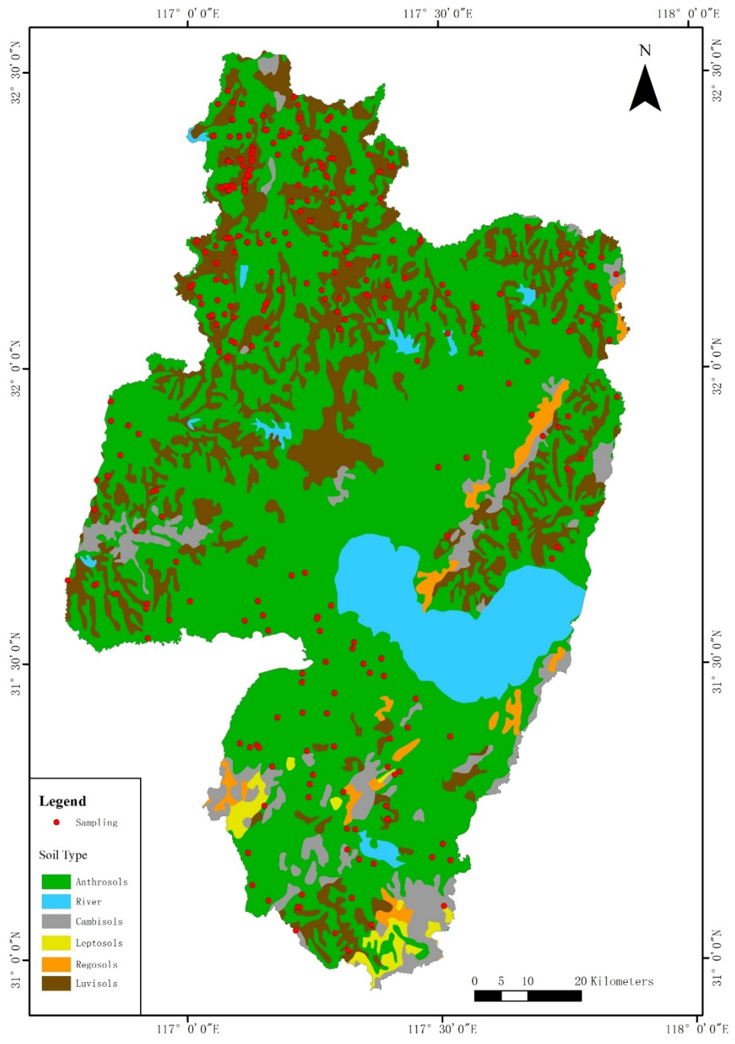
2.1. Overview of the Research Area
2.2. Soil Sample Source
2.3. Remote Sensing Data Processing
2.3.1. GF-6 Image Processing
2.3.2. Annual Maximum Synthetic Data
2.3.3. Terrain Data
2.4. Soil Type and Cultivated Land Planting Situation
2.5. Spatial Distance Data
2.6. Model Building and Testing
2.6.1. Model Introduction
- RF model: The RF algorithm is an ensemble learning method proposed by Breiman in 2001 [62]. The model is a bagged algorithm that contains multiple decision trees. The performance of a single regression tree is improved by combining multiple decision trees. The model output is the result of the integration of multiple decision trees.
- GBDT model: The GBDT model is a combination of decision tree and boosting algorithms and was proposed by Friedman in 2001 [63]. The model is an integrated tree model that calculates the residuals between the actual and predicted values. The integrated algorithm model uses gradient, boosting, and decision tree to solve the classification problem and perform the regression prediction. Boosting refers to the offline combination of multiple weak classifiers to achieve a strong classifier, and gradient refers to the increase in flexibility and convenience when the model solves the loss function. Compared to the support vector machine model, the GBDT algorithm has fewer model parameters, faster calculation speed, and higher stability.
- LightGBM model: As a part of the GBDT algorithm framework, LightGBM [64] internally integrates multiple decision trees and can integrate the decision results of multiple decision trees, avoiding the low accuracy shortcoming of the use of a single learning machine. The LightGBM algorithm adopts a leaf-wise growth strategy based on histograms, depth limitations, and exclusive feature bundling to increase the speed of calculation and improve training efficiency.
- XGBoost model: Chen and Guestrin proposed a new machine learning algorithm called the XGBoost algorithm in 2016 [65]. It has achieved excellent results in many international data mining competitions, and its performance exceeds that of deep learning algorithms [66,67]. The XGBoost algorithm improved on the GBDT algorithm. The loss function is determined by a second-order Taylor expansion, and the regularization concept of the loss function is introduced. The number of constrained nodes and outputs are added to the loss function, which makes the XGBoost algorithm more accurate than the GBDT algorithm, and the algorithm is hard to overfit.
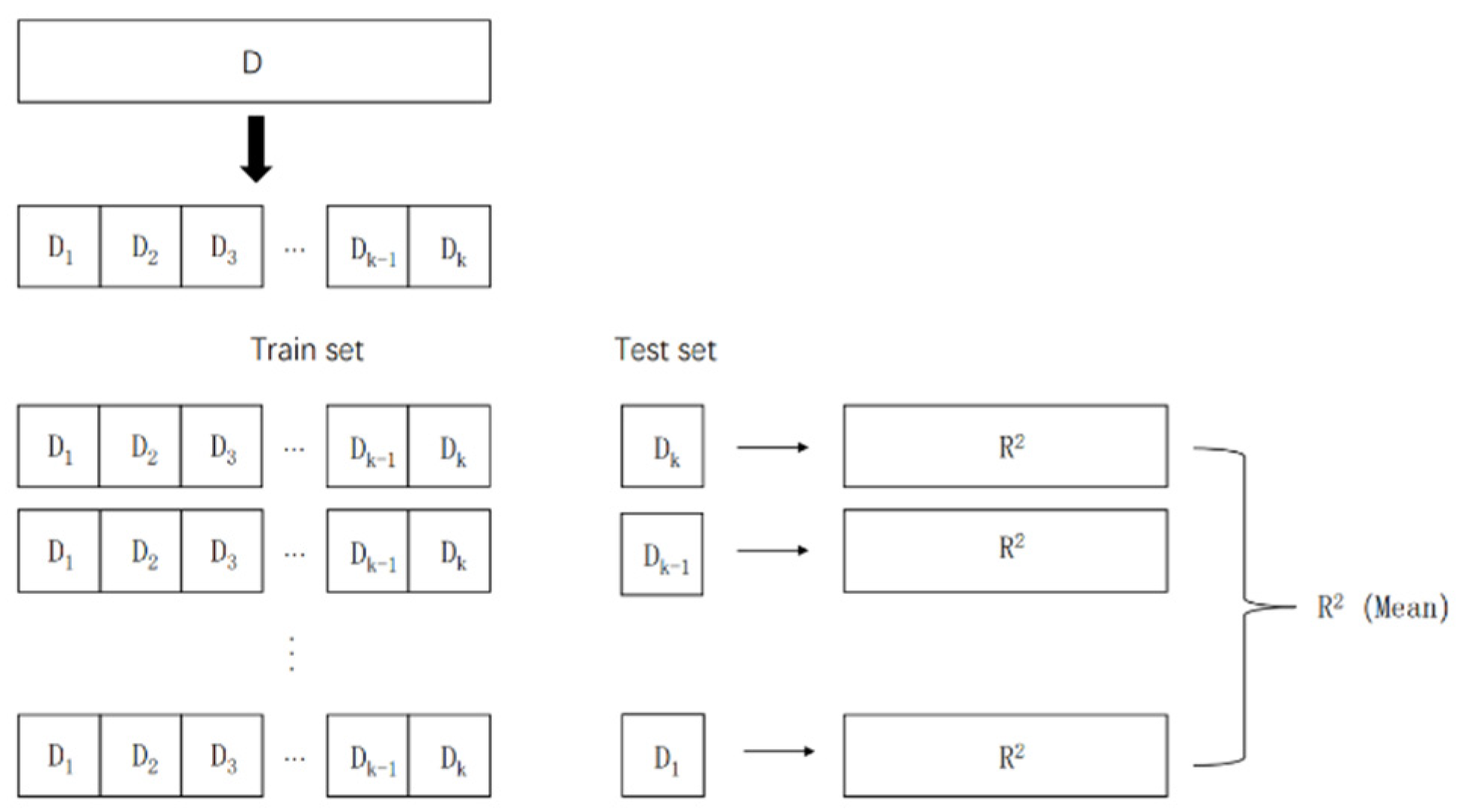
2.6.2. Model Evaluation and Tuning the Hyper-Parameters
3. Results
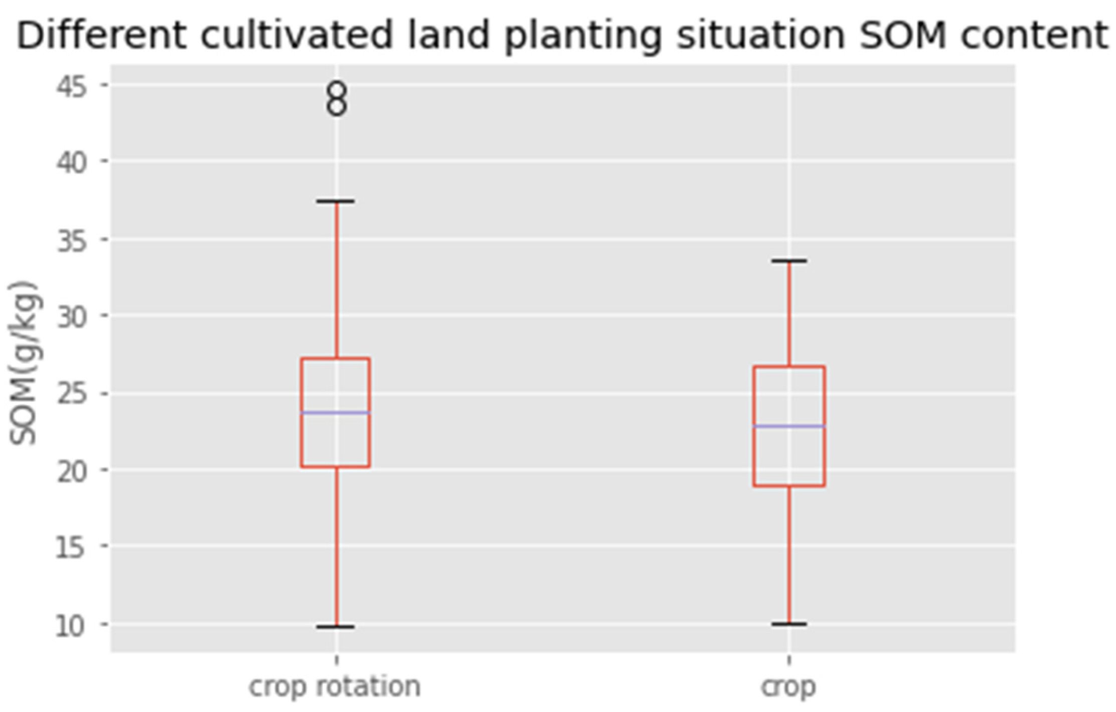
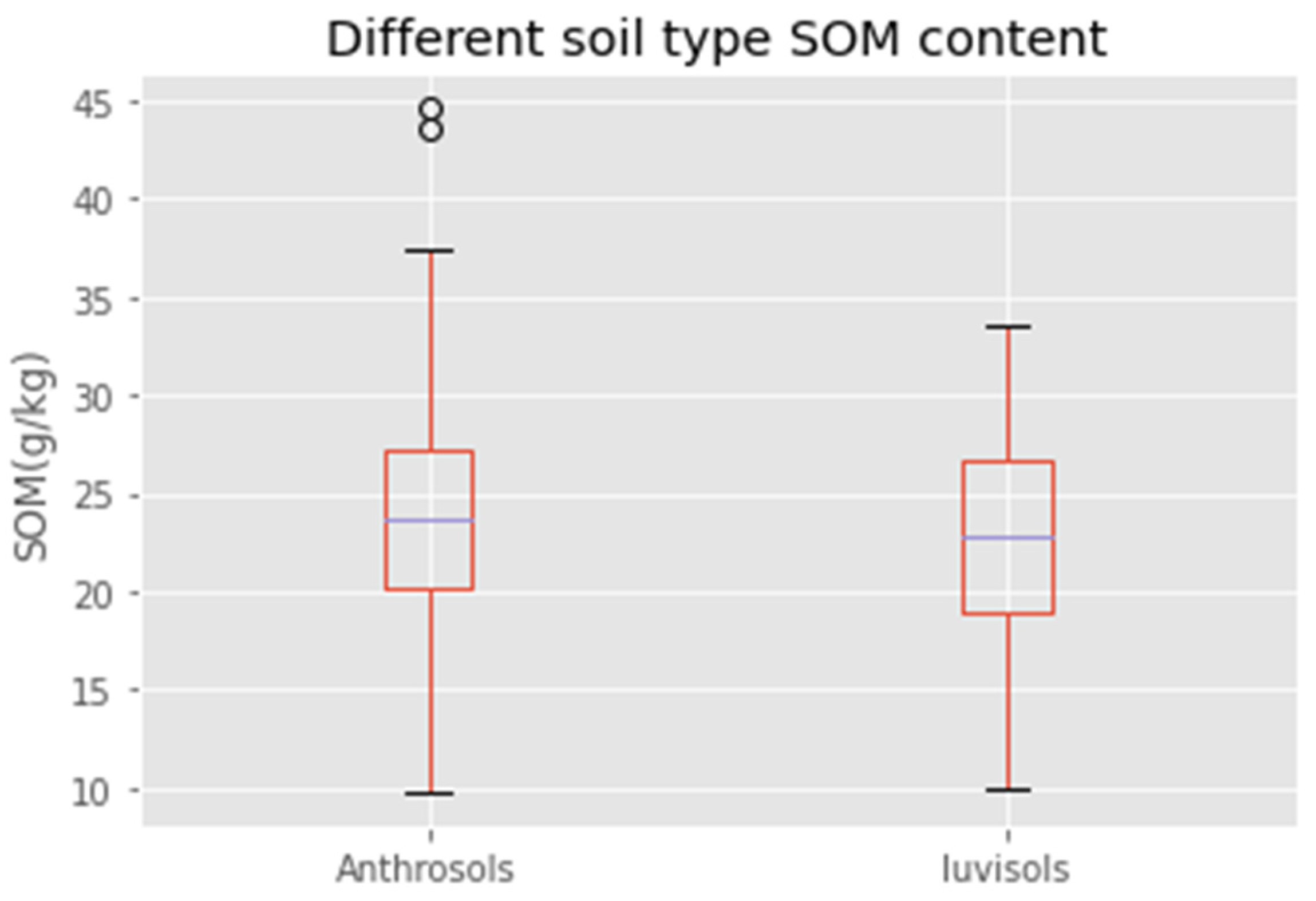
3.1. Statistical Analysis of Soil Organic Matter Content
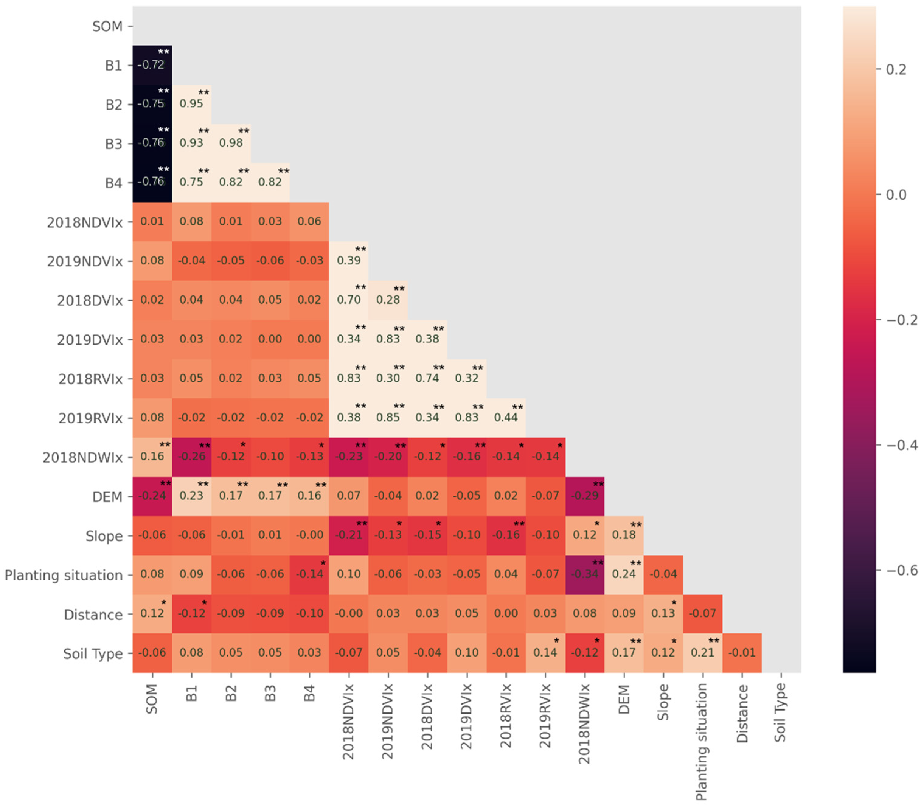
3.2. Correlation Analysis
3.3. Prediction Results of Surface Soil Organic Matter Content
3.3.1. Model Hyperparameter Selection
3.3.2. Evaluation of Model Calculation Speed
3.3.3. Model Accuracy Comparison
3.4. SOM Prediction Results of Different Datasets
3.4.1. Anthrosols Prediction Result
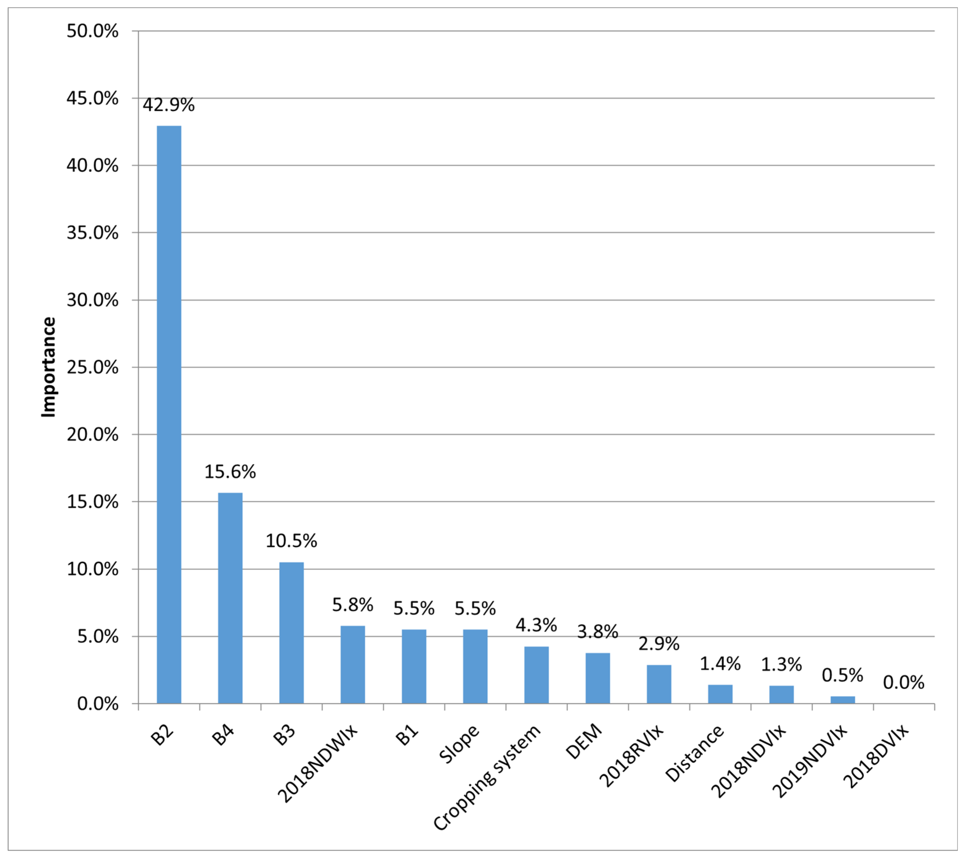
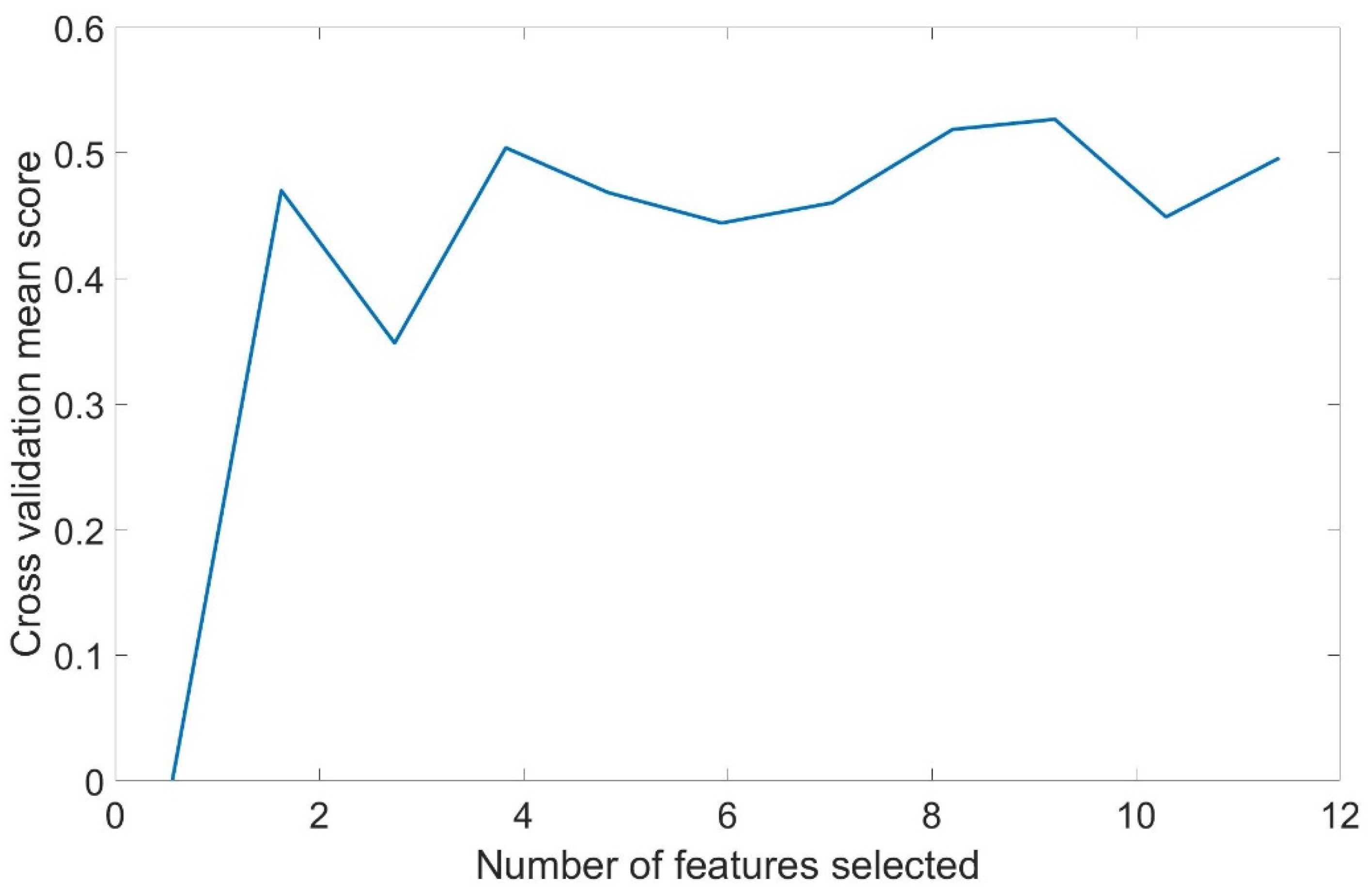
3.4.2. Feature Selection for Anthrosols Dataset
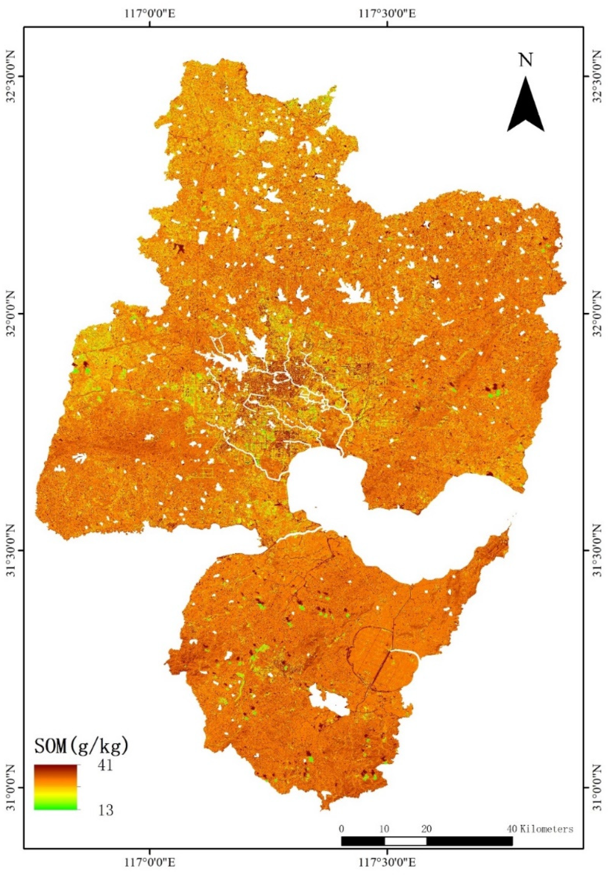
3.5. Simulation of the Spatial Distribution of SOM
4. Discussion
4.1. Predictive Performance Analysis
4.2. Selection and Optimization Analysis of Multivariate Data Features
4.3. GF-6 Modeling Advantage
4.4. Model Efficiency Analysis
4.5. Limitations of the Study
4.6. Model Selection
5. Conclusions
- (1)
- By comparing the R2, RMSE, and MAE values of each model, the XGBoost model was found to be the most suitable for predicting the spatial distribution of SOM in the study area. The R2, RMSE, and MAE values of the XGBoost model based on the optimized anthrosols dataset were 0.771, 1.773, and 1.474, respectively.
- (2)
- In terms of operating efficiency, the run times of the XGBoost, LightGBM, and GBDT models were shorter than those of the traditional RF model.
- (3)
- Machine learning methods such as XGBoost can achieve rapid and economical inversion of SOM content, allowing their application in precision agriculture.
Author Contributions
Funding
Institutional Review Board Statement
Informed Consent Statement
Data Availability Statement
Acknowledgments
Conflicts of Interest
Appendix A
References
- Mulla, D.J. Twenty five years of remote sensing in precision agriculture: Key advances and remaining knowledge gaps. Biosyst. Eng. 2013, 114, 358–371. [Google Scholar] [CrossRef]
- Lehmann, J.; Kleber, M. The contentious nature of soil organic matter. Nature 2015, 528, 60–68. [Google Scholar] [CrossRef] [PubMed]
- Kellerman, A.M.; Kothawala, D.N.; Dittmar, T.; Tranvik, L.J. Persistence of dissolved organic matter in lakes related to its molecular characteristics. Nat. Geosci. 2015, 8, 454–457. [Google Scholar] [CrossRef]
- Tuomisto, H.L.; Hodge, I.D.; Riordan, P.; Macdonald, D.W. Does organic farming reduce environmental impacts A meta-analysis of European research. J. Environ. Manag. 2012, 112, 309–320. [Google Scholar] [CrossRef]
- Berhe, A.A.; Barnes, R.T.; Six, J.; Marin-Spiotta, E. Role of Soil Erosion in Biogeochemical Cycling of Essential Elements: Carbon, Nitrogen, and Phosphorus. Annu. Rev. Earth Planet. Sci. 2018, 46, 521–548. [Google Scholar] [CrossRef]
- Kaiser, K.; Kalbitz, K. Cycling downwards—dissolved organic matter in soils. Soil Biol. Biochem. 2012, 52, 29–32. [Google Scholar] [CrossRef]
- Melillo, J.M.; Frey, S.D.; DeAngelis, K.M.; Werner, W.J.; Bernard, M.J.; Bowles, F.P.; Pold, G.; Knorr, M.A.; Grandy, A.S. Long-term pattern and magnitude of soil carbon feedback to the climate system in a warming world. Science 2017, 358, 101–104. [Google Scholar] [CrossRef] [Green Version]
- Caulfield, M.E.; Fonte, S.J.; Tittonell, P.; Vanek, S.J.; Sherwood, S.; Oyarzun, P.; Borja, R.M.; Dumble, S.; Groot, J.C.J. Inter-community and on-farm asymmetric organic matter allocation patterns drive soil fertility gradients in a rural Andean landscape. Land Degrad. Dev. 2020, 31, 2973–2985. [Google Scholar] [CrossRef]
- Wang, Y.; Liu, G.; Zhao, Z. Spatial heterogeneity of soil fertility in coastal zones: A case study of the Yellow River Delta, China. J. Soils Sediments 2021, 21, 1826–1839. [Google Scholar] [CrossRef]
- Jiang, Z.; Lian, F.; Wang, Z.; Xing, B. The role of biochars in sustainable crop production and soil resiliency. J. Exp. Bot. 2020, 71, 520–542. [Google Scholar] [CrossRef]
- Ramesh, T.; Bolan, N.S.; Kirkham, M.B.; Wijesekara, H.; Kanchikerimath, M.; Rao, C.S.; Sandeep, S.; Rinklebe, J.; Ok, Y.S.; Choudhury, B.U.; et al. Soil organic carbon dynamics: Impact of land use changes and management practices: A review. In Advances in Agronomy; Sparks, D.L., Ed.; Academic Press: Cambridge, MA, USA, 2012; Volume 156, pp. 1–107. [Google Scholar]
- Velasquez, E.; Lavelle, P. Soil macrofauna as an indicator for evaluating soil based ecosystem services in agricultural landscapes. Acta Oecolog. Int. J. Ecol. 2019, 100, 103446. [Google Scholar] [CrossRef]
- Oldfield, E.E.; Wood, S.A.; Bradford, M.A. Direct effects of soil organic matter on productivity mirror those observed with organic amendments. Plant Soil 2018, 423, 363–373. [Google Scholar] [CrossRef]
- Zhao, Y.N.; He, X.H.; Huang, X.C.; Zhang, Y.Q.; Shi, X.J. Increasing Soil Organic Matter Enhances Inherent Soil Productivity while Offsetting Fertilization Effect under a Rice Cropping System. Sustainability 2016, 8, 879. [Google Scholar] [CrossRef] [Green Version]
- Yuan, X.; Chai, X.; Gao, R.; He, Y.; Jin, H.; Huang, Y. Temporal and spatial variability of soil organic matter in a county scale agricultural ecosystem. N. Z. J. Agric. Res. 2007, 50, 1157–1168. [Google Scholar] [CrossRef] [Green Version]
- Hu, K.; Wang, S.; Li, H.; Huang, F.; Li, B. Spatial scaling effects on variability of soil organic matter and total nitrogen in suburban Beijing. Geoderma 2014, 226, 54–63. [Google Scholar] [CrossRef]
- Huang, B.; Sun, W.; Zhao, Y.; Zhu, J.; Yang, R.; Zou, Z.; Ding, F.; Su, J. Temporal and spatial variability of soil organic matter and total nitrogen in an agricultural ecosystem as affected by farming practices. Geoderma 2007, 139, 336–345. [Google Scholar] [CrossRef]
- van Beers, W.C.M.; Kleijnen, J.P.C. Kriging for interpolation in random simulation. J. Oper. Res. Soc. 2003, 54, 255–262. [Google Scholar] [CrossRef]
- López-Granados, F.; Jurado-Expósito, M.; Peña-Barragán, J.M.; García-Torres, L. Using geostatistical and remote sensing approaches for mapping soil properties. Eur. J. Agron. 2005, 23, 279–289. [Google Scholar] [CrossRef]
- Pouladi, N.; Møller, A.B.; Tabatabai, S.; Greve, M.H. Mapping soil organic matter contents at field level with Cubist, Random Forest and kriging. Geoderma 2019, 342, 85–92. [Google Scholar] [CrossRef]
- Henderson, T.L.; Szilagyi, A.; Baumgardner, M.F.; Chen, C.-C.T.; Landgrebe, D.A. Spectral Band Selection for Classification of Soil Organic Matter Content. Soil Sci. Soc. Am. J. 1989, 53, 1778–1784. [Google Scholar] [CrossRef]
- Zhang, M.; Zhang, M.; Yang, H.; Jin, Y.; Zhang, X.; Liu, H. Mapping Regional Soil Organic Matter Based on Sentinel-2A and MODIS Imagery Using Machine Learning Algorithms and Google Earth Engine. Remote. Sens. 2021, 13, 2934. [Google Scholar] [CrossRef]
- Santaga, F.S.; Agnelli, A.; Leccese, A.; Vizzari, M. Using Sentinel-2 for Simplifying Soil Sampling and Mapping: Two Case Studies in Umbria, Italy. Remote Sens. 2021, 13, 3379. [Google Scholar] [CrossRef]
- Meng, X.; Bao, Y.; Ye, Q.; Liu, H.; Zhang, X.; Tang, H.; Zhang, X. Soil Organic Matter Prediction Model with Satellite Hyperspectral Image Based on Optimized Denoising Method. Remote Sens. 2021, 13, 2273. [Google Scholar] [CrossRef]
- Nanni, M.R.; Demattê, J.A.; Rodrigues, M.; Santos, G.L.; Reis, A.S.; Oliveira, K.M.; Cezar, E.; Furlanetto, R.H.; Crusiol, L.G.; Sun, L. Mapping Particle Size and Soil Organic Matter in Tropical Soil Based on Hyperspectral Imaging and Non-Imaging Sensors. Remote Sens. 2021, 13, 1782. [Google Scholar] [CrossRef]
- Gomez, C.; Rossel, R.A.V.; McBratney, A.B. Soil organic carbon prediction by hyperspectral remote sensing and field vis-NIR spectroscopy: An Australian case study. Geoderma 2008, 146, 403–411. [Google Scholar] [CrossRef]
- Li, X.-P.; Zhang, F.; Wang, X.-P. Study on Differential-Based Multispectral Modeling of Soil Organic Matter in Ebinur Lake Wetland. Spectrosc. Spectr. Anal. 2019, 39, 535–542. [Google Scholar] [CrossRef]
- Zhai, M. Inversion of organic matter content in wetland soil based on Landsat 8 remote sensing image. J. Vis. Commun. Image Represent. 2019, 64, 102645. [Google Scholar] [CrossRef]
- Baumgardner, M.F.; Kristof, S.; Johannsen, C.J.; Zachary, A. Effects of organic matter on the multispectral properties of soils. Proc. Indiana Acad. Sci. 1969, 79, 413–422. [Google Scholar]
- Chen, Y.; Zhang, M.; Fan, D.; Fan, K.; Wang, X. Linear Regression between CIE-Lab Color Parameters and Organic Matter in Soils of Tea Plantations. Eurasian Soil Sci. 2018, 51, 199–203. [Google Scholar] [CrossRef]
- Kodaira, M.; Shibusawa, S. Using a mobile real-time soil visible-near infrared sensor for high resolution soil property mapping. Geoderma 2013, 199, 64–79. [Google Scholar] [CrossRef]
- Rodionov, A.; Welp, G.; Damerow, L.; Berg, T.; Amelung, W.; Paetzold, S. Towards on-the-go field assessment of soil organic carbon using Vis-NIR diffuse reflectance spectroscopy: Developing and testing a novel tractor-driven measuring chamber. Soil Tillage Res. 2015, 145, 93–102. [Google Scholar] [CrossRef]
- Biney, J.K.M.; Boruvka, L.; Chapman Agyeman, P.; Nemecek, K.; Klement, A. Comparison of Field and Laboratory Wet Soil Spectra in the Vis-NIR Range for Soil Organic Carbon Prediction in the Absence of Laboratory Dry Measurements. Remote Sens. 2020, 12, 3082. [Google Scholar] [CrossRef]
- Rasul, A.; Balzter, H.; Ibrahim, G.R.F.; Hameed, H.M.; Wheeler, J.; Adamu, B.; Ibrahim, S.a.; Najmaddin, P.M. Applying built-up and bare-soil indices from Landsat 8 to cities in dry climates. Land 2018, 7, 81. [Google Scholar] [CrossRef] [Green Version]
- Xu, C.; Qu, J.J.; Hao, X.; Cosh, M.H.; Prueger, J.H.; Zhu, Z.; Gutenberg, L. Downscaling of surface soil moisture retrieval by combining MODIS/Landsat and in situ measurements. Remote Sens. 2018, 10, 210. [Google Scholar] [CrossRef] [Green Version]
- Zhang, Y.; Guo, L.; Chen, Y.; Shi, T.; Luo, M.; Ju, Q.; Zhang, H.; Wang, S. Prediction of Soil Organic Carbon based on Landsat 8 Monthly NDVI Data for the Jianghan Plain in Hubei Province, China. Remote Sens. 2019, 11, 1683. [Google Scholar] [CrossRef] [Green Version]
- Yu, H.; Liu, M.; Du, B.; Wang, Z.; Hu, L.; Zhang, B. Mapping Soil Salinity/Sodicity by using Landsat OLI Imagery and PLSR Algorithm over Semiarid West Jilin Province, China. Sensors 2018, 18, 1048. [Google Scholar] [CrossRef] [Green Version]
- Fu, C.; Gan, S.; Yuan, X.; Xiong, H.; Tian, A. Impact of Fractional Calculus on Correlation Coefficient between Available Potassium and Spectrum Data in Ground Hyperspectral and Landsat 8 Image. Mathematics 2019, 7, 488. [Google Scholar] [CrossRef] [Green Version]
- Seema; Ghosh, A.K.; Das, B.S.; Reddy, N. Application of VIS-NIR spectroscopy for estimation of soil organic carbon using different spectral preprocessing techniques and multivariate methods in the middle Indo-Gangetic plains of India. Geoderma Reg. 2020, 23, e00349. [Google Scholar] [CrossRef]
- Dou, X.; Wang, X.; Liu, H.; Zhang, X.; Meng, L.; Pan, Y.; Yu, Z.; Cui, Y. Prediction of soil organic matter using multi-temporal satellite images in the Songnen Plain, China. Geoderma 2019, 356, 113896. [Google Scholar] [CrossRef]
- Cao, X.; Li, X.; Ren, W.; Wu, Y.; Liu, J. Hyperspectral estimation of soil organic matter content using grey relational local regression model. Grey Syst.Theory Appl. 2020, 11, 707–722. [Google Scholar] [CrossRef]
- Costa, E.M.; Tassinari, W.d.S.; Koenow Pinheiro, H.S.; Beutler, S.J.; Cunha dos Anjos, L.H. Mapping Soil Organic Carbon and Organic Matter Fractions by Geographically Weighted Regression. J. Environ. Qual. 2018, 47, 718–725. [Google Scholar] [CrossRef]
- Takata, Y.; Funakawa, S.; Akshalov, K.; Ishida, N.; Kosaki, T. Spatial prediction of soil organic matter in northern Kazakhstan based on topographic and vegetation information. Soil Sci. Plant Nutr. 2007, 53, 289–299. [Google Scholar] [CrossRef]
- Emadi, M.; Taghizadeh-Mehrjardi, R.; Cherati, A.; Danesh, M.; Mosavi, A.; Scholten, T. Predicting and Mapping of Soil Organic Carbon Using Machine Learning Algorithms in Northern Iran. Remote Sens. 2020, 12, 2234. [Google Scholar] [CrossRef]
- Kobayashi, Y.; Yoshida, K. Quantitative structure?property relationships for the calculation of the soil adsorption coefficient using machine learning algorithms with calculated chemical properties from open-source software. Environ. Res. 2021, 196. [Google Scholar] [CrossRef]
- Dong, Z.; Wang, N.; Liu, J.; Xie, J.; Han, J. Combination of machine learning and VIRS for predicting soil organic matter. J. Soils Sediments 2021, 21, 2578–2588. [Google Scholar] [CrossRef]
- Wang, X.; Han, J.; Wang, X.; Yao, H.; Zhang, L. Estimating Soil Organic Matter Content Using Sentinel-2 Imagery by Machine Learning in Shanghai. IEEE Access 2021, 9, 78215–78225. [Google Scholar] [CrossRef]
- Wang, Z.; Du, Z.; Li, X.; Bao, Z.; Zhao, N.; Yue, T. Incorporation of high accuracy surface modeling into machine learning to improve soil organic matter mapping. Ecol. Indic. 2021, 129, 107975. [Google Scholar] [CrossRef]
- Yang, J.; Li, X.; Wu, B.; Wu, J.; Sun, B.; Yan, C.; Gao, Z. High Spatial Resolution Topsoil Organic Matter Content Mapping Across Desertified Land in Northern China. Front. Environ. Sci. 2021, 9, 668912. [Google Scholar] [CrossRef]
- Hong, Y.; Liu, Y.; Chen, Y.; Liu, Y.; Yu, L.; Liu, Y.; Cheng, H. Application of fractional-order derivative in the quantitative estimation of soil organic matter content through visible and near-infrared spectroscopy. Geoderma 2019, 337, 758–769. [Google Scholar] [CrossRef]
- Wang, Z.; Wang, G.; Zhang, G.; Wang, H.; Ren, T. Effects of land use types and environmental factors on spatial distribution of soil total nitrogen in a coalfield on the Loess Plateau, China. Soil Tillage Res. 2021, 211, 105027. [Google Scholar] [CrossRef]
- Bokde, N.D.; Ali, Z.H.; Al-Hadidi, M.T.; Farooque, A.A.; Jamei, M.; Al Maliki, A.A.; Beyaztas, B.H.; Faris, H.; Yaseen, Z.M. Total Dissolved Salt Prediction Using Neurocomputing Models: Case Study of Gypsum Soil Within Iraq Region. IEEE Access 2021, 9, 53617–53635. [Google Scholar] [CrossRef]
- Liu, L.; Ji, M.; Buchroithner, M. Combining Partial Least Squares and the Gradient-Boosting Method for Soil Property Retrieval Using Visible Near-Infrared Shortwave Infrared Spectra. Remote Sens. 2017, 9, 1299. [Google Scholar] [CrossRef] [Green Version]
- Wang, Z.; Wang, G.; Zhang, Y.; Wang, R. Quantification of the effect of soil erosion factors on soil nutrients at a small watershed in the Loess Plateau, Northwest China. J. Soils Sediments 2020, 20, 745–755. [Google Scholar] [CrossRef]
- Ahirwal, J.; Nath, A.; Brahma, B.; Deb, S.; Sahoo, U.K.; Nath, A.J. Patterns and driving factors of biomass carbon and soil organic carbon stock in the Indian Himalayan region. Sci. Total Environ. 2021, 770, 145292. [Google Scholar] [CrossRef] [PubMed]
- Jiang, G.; Grafton, M.; Pearson, D.; Bretherton, M.; Holmes, A. Predicting spatiotemporal yield variability to aid arable precision agriculture in New Zealand: A case study of maize-grain crop production in the Waikato region. N. Z. J. Crop. Hortic. Sci. 2021, 49, 41–62. [Google Scholar] [CrossRef]
- Li, M.; Xi, X.; Xiao, G.; Cheng, H.; Yang, Z.; Zhou, G.; Ye, J.; Li, Z. National multi-purpose regional geochemical survey in China. J. Geochem. Explor. 2014, 139, 21–30. [Google Scholar] [CrossRef]
- Tian, F.; Wang, Y.; Fensholt, R.; Wang, K.; Zhang, L.; Huang, Y. Mapping and Evaluation of NDVI Trends from Synthetic Time Series Obtained by Blending Landsat and MODIS Data around a Coalfield on the Loess Plateau. Remote Sens. 2013, 5, 4255–4279. [Google Scholar] [CrossRef] [Green Version]
- Ma, Y.; Liu, H.; Jiang, B.; Meng, L.; Guan, H.; Xu, M.; Cui, Y.; Kong, F.; Yin, Y.; Wang, M. An Innovative Approach for Improving the Accuracy of Digital Elevation Models for Cultivated Land. Remote Sens. 2020, 12, 3401. [Google Scholar] [CrossRef]
- Busch, R.; Hardt, J.; Nir, N.; Schuett, B. Modeling Gully Erosion Susceptibility to Evaluate Human Impact on a Local Landscape System in Tigray, Ethiopia. Remote Sens. 2021, 13, 2009. [Google Scholar] [CrossRef]
- Zhao, C.; Zhou, Y.; Jiang, J.H.; Xiao, P.N.; Wu, H. Spatial characteristics of cultivated land quality accounting for ecological environmental condition: A case study in hilly area of northern Hubei province, China. Sci. Total Environ. 2021, 774, 145765. [Google Scholar] [CrossRef]
- Breiman, L. Random forests. Mach. Learn. 2001, 45, 5–32. [Google Scholar] [CrossRef] [Green Version]
- Friedman, J.H. Greedy function approximation: A gradient boosting machine. Ann. Stat. 2001, 29, 1189–1232. [Google Scholar] [CrossRef]
- Ma, X.; Sha, J.; Wang, D.; Yu, Y.; Yang, Q.; Niu, X. Study on a prediction of P2P network loan default based on the machine learning LightGBM and XGboost algorithms according to different high dimensional data cleaning. Electron. Commer. Res. Appl. 2018, 31, 24–39. [Google Scholar] [CrossRef]
- Chen, T.; Guestrin, C. XGBoost: A scalable tree boosting system. In Proceedings of the 22nd ACM SIGKDD International Conference on Knowledge Discovery and Data Mining, San Francisco, CA, USA, 13–17 August 2016; Volume 10, pp. 785–794. [Google Scholar]
- Giannakas, F.; Troussas, C.; Krouska, A.; Sgouropoulou, C.; Voyiatzis, I. XGBoost and Deep Neural Network Comparison: The Case of Teams’ Performance. In International Conference on Intelligent Tutoring Systems; Springer: Cham, Switzerland, 2021; pp. 343–349. [Google Scholar]
- Zamani Joharestani, M.; Cao, C.; Ni, X.; Bashir, B.; Talebiesfandarani, S. PM2.5 Prediction Based on Random Forest, XGBoost, and Deep Learning Using Multisource Remote Sensing Data. Atmosphere 2019, 10, 373. [Google Scholar] [CrossRef] [Green Version]
- Zhou, L.; Luo, T.; Du, M.; Chen, Q.; Liu, Y.; Zhu, Y.; He, C.; Wang, S.; Yang, K. Machine Learning Comparison and Parameter Setting Methods for the Detection of Dump Sites for Construction and Demolition Waste Using the Google Earth Engine. Remote Sens. 2021, 13, 787. [Google Scholar] [CrossRef]
- Zhang, Y.; Ma, J.; Liang, S.; Li, X.; Li, M. An Evaluation of Eight Machine Learning Regression Algorithms for Forest Aboveground Biomass Estimation from Multiple Satellite Data Products. Remote Sens. 2020, 12, 4015. [Google Scholar] [CrossRef]
- Ramezan, C.; Warner, T.; Maxwell, A. Evaluation of Sampling and Cross-Validation Tuning Strategies for Regional-Scale Machine Learning Classification. Remote Sens. 2019, 11, 185. [Google Scholar] [CrossRef] [Green Version]
- Wang, Z.; Hu, M.; Zhai, G. Application of Deep Learning Architectures for Accurate and Rapid Detection of Internal Mechanical Damage of Blueberry Using Hyperspectral Transmittance Data. Sensors 2018, 18, 1126. [Google Scholar] [CrossRef] [Green Version]
- Fan, M.; Lal, R.; Zhang, H.; Margenot, A.J.; Wu, J.; Wu, P.; Zhang, L.; Yao, J.; Chen, F.; Gao, C. Variability and determinants of soil organic matter under different land uses and soil types in eastern China. Soil Tillage Res. 2020, 198, 104544. [Google Scholar] [CrossRef]
- Zhisheng, A.; Tunghseng, L.; Yanchou, L.; Porter, S.C.; Kukla, G.; Xihao, W.; Yingming, H. The long-term paleomonsoon variation recorded by the loess-paleosol sequence In central China. Quat. Int. 1990, 7, 91–95. [Google Scholar] [CrossRef]
- Villamil-Cubillos, L.F.; Leon-Medina, J.X.; Anaya, M.; Tibaduiza, D.A. Evaluation of Feature Selection Techniques in a Multifrequency Large Amplitude Pulse Voltammetric Electronic Tongue. Eng. Proc. 2020, 2, 62. [Google Scholar] [CrossRef]
- Zhang, W.; Wu, C.; Zhong, H.; Li, Y.; Wang, L. Prediction of undrained shear strength using extreme gradient boosting and random forest based on Bayesian optimization. Geosci. Front. 2021, 12, 469–477. [Google Scholar] [CrossRef]
- Guo, N.; Shi, X.; Zhao, Y.; Xu, S.; Wang, M.; Zhang, G.; Wu, J.; Huang, B.; Kong, C. Environmental and anthropogenic factors driving changes in paddy soil organic matter: A case study in the Middle and Lower Yangtze River Plain of China. Pedosphere 2017, 27, 926–937. [Google Scholar] [CrossRef]
- Duan, L.; Li, Z.; Xie, H.; Li, Z.; Zhang, L.; Zhou, Q. Large-scale spatial variability of eight soil chemical properties within paddy fields. Catena 2020, 188, 104350. [Google Scholar] [CrossRef]
- Wang, H.; Zhang, X.; Wu, W.; Liu, H. Prediction of Soil Organic Carbon under Different Land Use Types Using Sentinel-1/-2 Data in a Small Watershed. Remote Sens. 2021, 13, 1229. [Google Scholar] [CrossRef]
- Li, Z.Q.; Zhang, X.; Xu, J.; Cao, K.; Wang, J.H.; Xu, C.X.; Cao, W.D. Green manure incorporation with reductions in chemical fertilizer inputs improves rice yield and soil organic matter accumulation. J. Soils Sediments 2020, 20, 2784–2793. [Google Scholar] [CrossRef]
- Du, Z.; Gao, B.; Ou, C.; Du, Z.; Yang, J.; Batsaikhan, B.; Dorjgotov, B.; Yun, W.; Zhu, D. A Quantitative Analysis of Factors Influencing Organic Matter Concentration in the Topsoil of Black Soil in Northeast China Based on Spatial Heterogeneous Patterns. ISPRS Int. J. Geo-Inf. 2021, 10, 348. [Google Scholar] [CrossRef]
- Sheng, Y.; Liu, W.; Xu, H.; Gao, X. The Spatial Distribution Characteristics of the Cultivated Land Quality in the Diluvial Fan Terrain of the Arid Region: A Case Study of Jimsar County, Xinjiang, China. Land 2021, 10, 896. [Google Scholar] [CrossRef]
- Sahabiev, I.; Smirnova, E.; Giniyatullin, K. Spatial Prediction of Agrochemical Properties on the Scale of a Single Field Using Machine Learning Methods Based on Remote Sensing Data. Agronomy 2021, 11, 2266. [Google Scholar] [CrossRef]
- Wang, X.; Shi, W.; Sun, X.; Wang, M. Comprehensive benefits evaluation and its spatial simulation for well-facilitated farmland projects in the Huang-Huai-Hai Region of China. Land Degrad. Dev. 2020, 31, 1837–1850. [Google Scholar] [CrossRef]
- Szegedy, C.; Liu, W.; Jia, Y.; Sermanet, P.; Reed, S.; Anguelov, D.; Erhan, D.; Vanhoucke, V.; Rabinovich, A. Going deeper with convolutions. In Proceedings of the IEEE Conference on Computer Vision and Pattern Recognition, Boston, MA, USA, 8–10 June 2015; pp. 1–9. [Google Scholar]
- Ciresan, D.; Giusti, A.; Gambardella, L.; Schmidhuber, J. Deep neural networks segment neuronal membranes in electron microscopy images. Adv. Neural Inf. Process. Syst. 2012, 25, 2843–2851. [Google Scholar]
- Montavon, G.; Lapuschkin, S.; Binder, A.; Samek, W.; Müller, K.-R. Explaining nonlinear classification decisions with deep Taylor decomposition. Pattern Recognit. 2017, 65, 211–222. [Google Scholar] [CrossRef]


| Band | Range (μm) |
|---|---|
| B1 | 0.45–0.52 |
| B2 | 0.52–0.60 |
| B3 | 0.63–0.69 |
| B4 | 0.76–0.90 |
| Name of Dataset | Dataset | Resolution | Source |
|---|---|---|---|
| Soil reflectance data | B1-B4 | 8 m | GF-6 |
| Google Earth Engine (GEE) maximum annual indices | 2018NDWIx | 8 m | Landsat8 |
| 2018NDVIx | 8 m | ||
| 2019NDVIx | 8 m | ||
| 2018DVIx | 8 m | ||
| 2019DVIx | 8 m | ||
| 2018RVIx | 8 m | ||
| 2019RVIx | 8 m | ||
| GEE digital elevation model (DEM) data | DEM | 30 m | Shuttle Radar Topography Mission (SRTM) |
| Slope | 30 m | ||
| Soil and cultivated land planting situation | Soil type | Vector data | Department of agriculture |
| cultivated land planting situation | Vector data | ||
| Geostatistical data | Distance | Vector data | Department of natural resources |
| Sampling Dataset | N | SOM | ||||||
|---|---|---|---|---|---|---|---|---|
| Max | Min | Mean | Standard Deviation | Kurtosis | Skewness | Coefficient of Variation | ||
| Whole sampling | 295 | 44.6 | 9.8 | 23.19 | 5.894 | 0.384 | 0.048 | 0.254 |
| Anthrosols | 204 | 44.6 | 9.8 | 23.45 | 6.023 | 0.578 | 0.145 | 0.257 |
| Luvisols | 84 | 33.5 | 9.9 | 22.52 | 5.690 | −0.477 | −0.230 | 0.253 |
| Regression Model | Hyperparameters | Optimal Parameter | Default Parameters | Range of Grid Search |
|---|---|---|---|---|
| Extreme gradient boosting machine (XGBoost) | random_state | 0 | 0 | 0 |
| n_estimators | 15 | 100 | 0~100 | |
| max_depth | 2 | 6 | 1~10 | |
| learning_rate | 0.38 | 0.3 | 0.01~1.00 | |
| min_child_weight | 4 | 1 | 1~10 | |
| gamma | 0.1 | 0 | 0~1.0 | |
| Light gradient boosting machine (LightGBM) | random_state | 0 | None | 0 |
| n_estimators | 26 | 100 | 0~100 | |
| max_depth | 7 | −1 | 1~10 | |
| learning_rate | 0.1 | 0.1 | 0.01~1.00 | |
| subsample | 0.1 | 1 | 0~1.0 | |
| Gradient boosting tree (GBDT) | random_state | 0 | None | 0 |
| n_estimators | 21 | 100 | 0~100 | |
| max_depth | 4 | 3 | 1~10 | |
| learning_rate | 0.18 | 0.1 | 0.01~1.00 | |
| Random Forest (RF) | random_state | 0 | None | 0 |
| n_estimators | 83 | 100 | 0~100 | |
| max_depth | 8 | None | 1~10 | |
| min_samples_split | 9 | 2 | 1~10 | |
| min_samples_leaf | 1 | 1 | 1~10 |
| Regression Model | Runtime (s) |
|---|---|
| XGBoost | 0.2 |
| LightGBM | 0.1 |
| GBDT | 0.3 |
| RF | 1.4 |
| Regression Model | Performance Indicator | ||
|---|---|---|---|
| Coefficient of Determination (R2) | Root Mean Square Error (RMSE) | Mean Absolute Error (MAE) | |
| XGBoost | 0.634 | 3.250 | 2.637 |
| LightGBM | 0.627 | 3.278 | 2.618 |
| GBDT | 0.591 | 3.432 | 2.780 |
| RF | 0.551 | 3.591 | 2.698 |
| Regression Model | Hyperparameters | Optimal Parameter |
|---|---|---|
| XGBoost | random_state | 0 |
| n_estimators | 14 | |
| max_depth | 2 | |
| LightGBM | random_state | 0 |
| n_estimators | 60 | |
| max_depth | 6 | |
| learning_rate | 0.08 | |
| subsample | 0.01 | |
| GBDT | random_state | 0 |
| n_estimators | 27 | |
| max_depth | 3 | |
| learning_rate | 0.11 | |
| RF | random_state | 0 |
| n_estimators | 89 | |
| max_depth | 9 | |
| min_samples_split | 3 | |
| min_samples_leaf | 1 |
| Regression Model | Runtimes (s) | Performance Indicator | ||
|---|---|---|---|---|
| R2 | RMSE | MAE | ||
| XGBoost | 0.2 | 0.748 | 1.858 | 1.405 |
| LightGBM | 0.2 | 0.355 | 2.974 | 2.198 |
| GBDT | 0.2 | 0.711 | 1.990 | 1.583 |
| RF | 1.4 | 0.741 | 1.880 | 1.649 |
| Regression Model | Runtime (s) | Performance Indicator | ||
|---|---|---|---|---|
| R2 | RMSE | MAE | ||
| XGBoost | 0.2 | 0.771 | 1.773 | 1.474 |
Publisher’s Note: MDPI stays neutral with regard to jurisdictional claims in published maps and institutional affiliations. |
© 2021 by the authors. Licensee MDPI, Basel, Switzerland. This article is an open access article distributed under the terms and conditions of the Creative Commons Attribution (CC BY) license (https://creativecommons.org/licenses/by/4.0/).
Share and Cite
Ye, Z.; Sheng, Z.; Liu, X.; Ma, Y.; Wang, R.; Ding, S.; Liu, M.; Li, Z.; Wang, Q. Using Machine Learning Algorithms Based on GF-6 and Google Earth Engine to Predict and Map the Spatial Distribution of Soil Organic Matter Content. Sustainability 2021, 13, 14055. https://doi.org/10.3390/su132414055
Ye Z, Sheng Z, Liu X, Ma Y, Wang R, Ding S, Liu M, Li Z, Wang Q. Using Machine Learning Algorithms Based on GF-6 and Google Earth Engine to Predict and Map the Spatial Distribution of Soil Organic Matter Content. Sustainability. 2021; 13(24):14055. https://doi.org/10.3390/su132414055
Chicago/Turabian StyleYe, Zhishan, Ziheng Sheng, Xiaoyan Liu, Youhua Ma, Ruochen Wang, Shiwei Ding, Mengqian Liu, Zijie Li, and Qiang Wang. 2021. "Using Machine Learning Algorithms Based on GF-6 and Google Earth Engine to Predict and Map the Spatial Distribution of Soil Organic Matter Content" Sustainability 13, no. 24: 14055. https://doi.org/10.3390/su132414055
APA StyleYe, Z., Sheng, Z., Liu, X., Ma, Y., Wang, R., Ding, S., Liu, M., Li, Z., & Wang, Q. (2021). Using Machine Learning Algorithms Based on GF-6 and Google Earth Engine to Predict and Map the Spatial Distribution of Soil Organic Matter Content. Sustainability, 13(24), 14055. https://doi.org/10.3390/su132414055