Designing a Resilient and Sustainable Logistics Network under Epidemic Disruptions and Demand Uncertainty

Abstract

To face the new challenges caused by modern industry, logistics operations managers need to focus more on integrating sustainability goals, adapt to unexpected disruptions and find new strategies and models for logistics management. The COVID-19 pandemic has proven that unforeseen fragilities, negatively affecting the supply chain performance, can arise rapidly, and logistics systems may confront unprecedented vulnerabilities regarding network structure disruption and high demand fluctuations. The existing studies on a resilient logistics network design did not sufficiently consider sustainability aspects. In fact, they mainly addressed the independent planning of decision-making problems with economic objectives. To fill this research gap, this paper concentrates on the design of resilient and sustainable logistics networks under epidemic disruption and demand uncertainty. A two-stage stochastic mixed integer programming model is proposed to integrate key decisions of location–allocation, inventory and routing planning. Moreover, epidemic disruptions and demand uncertainty are incorporated through plausible scenarios using a Monte Carlo simulation. In addition, two resiliency strategies, namely, capacity augmentation and logistics collaboration, are included into the basic model in order to improve the resilience and the sustainability of a logistics chain network. Finally, numerical examples are presented to validate the proposed approach, evaluate the performance of the different design models and provide managerial insights. The obtained results show that the integration of two design strategies improves resilience and sustainability.

1. Introduction

In recent years, supply chains have become more complex and very vulnerable to various disruptions [1,2,3,4]. As a result, logistics networks have confronted uncertainties significantly disrupt the supply chain operations [5,6]. The latter may be also influenced by natural disasters, strikes, fluctuations in the electrical system, economic or political crises and epidemic disruptions of infectious diseases [7,8,9,10]. For instance, the current COVID-19 outbreak has severely affected different domains, especially the freight transport sector, due to its rapid propagation [8,11,12]. In fact, disruption remarkably affects the entire logistics system [13]. For example, any disruption in one region may influence the neighboring or related regions. In addition, operational risks, caused by the inherent uncertainty of the data and the fluctuating nature of the input data, can more or less deteriorate the performance of the logistics systems [14]. Consequently, the epidemic disruption propagation and operational risks in the logistics network design have become key issues that should be dealt with in order to face uncertainty risks.

Recently, resilience has been studied by the research community as a strategic approach applied to design and evaluate logistics networks in order to avoid performance degradation and disruption propagation [15,16,17,18]. It is defined as the ability of the supply chains to quickly return to their ideal performance level and preserve the continuity of material flow after its interruption [19]. Indeed, resilience strategies can be classified into two types: reactive strategies or proactive strategies. The first ones, such as resource sharing and fortification of platforms, are implemented before the occurrence of disruptions. However, proactive strategies, like capacity expansion and backup suppliers, are applied after disruptions. Recent literature on supply chain resilience has shown that ripple effect disruptions, such as the COVID-19 pandemic, have a high considerable impact and low frequency that cascade downstream in the logistics network [20]. In addition, it has suggested that the supply chains, particularly logistics systems, need to move towards highly resilient logistics strategies and practices.

Along with the vulnerability of logistics chains, the concept of sustainable development has increasingly become, in the last few decades, an important strategic concern due to global competitiveness and tighter regulations in society [21,22,23,24]. Indeed, the logistics network should evolve to create sustainable and modern society. Despite a rich literature on logistics network planning, establishing sustainable logistics management with considered disruptions is still an important topic that has not yet been widely dealt with by researchers and industries. As a consequence, it is necessary to design effective strategies to overcome disruption risks and sustainability challenges.

Sustainability and resilience are two relatively new practices that seek new development and effectiveness improvement in the design and evaluation of logistics networks in a wider angle [25,26]. In fact, logistics network design includes strategic, tactical and operational decisions, namely, location decisions, transportation and inventory planning. These decisions are usually treated independently or sequentially [27]. However, as mentioned in several works of the literature [20,28], epidemic disruptions affect remarkably all planning decisions due to their ripple effects. Therefore, it is important to develop design models integrating the different planning decisions. This topic has been a recent trend and has proven to be highly effective in practice [29]. Moreover, the assessment of the performance of logistics configurations is based mainly on economic criteria and ignores environmental and social sustainability [30]. To the best of our knowledge, no attempt has been made to address the stochastic inventory-location-routing problem, considering both sustainability issues and epidemic disruptions. The main contributions of this paper that differentiate our efforts from related studies are as follows:

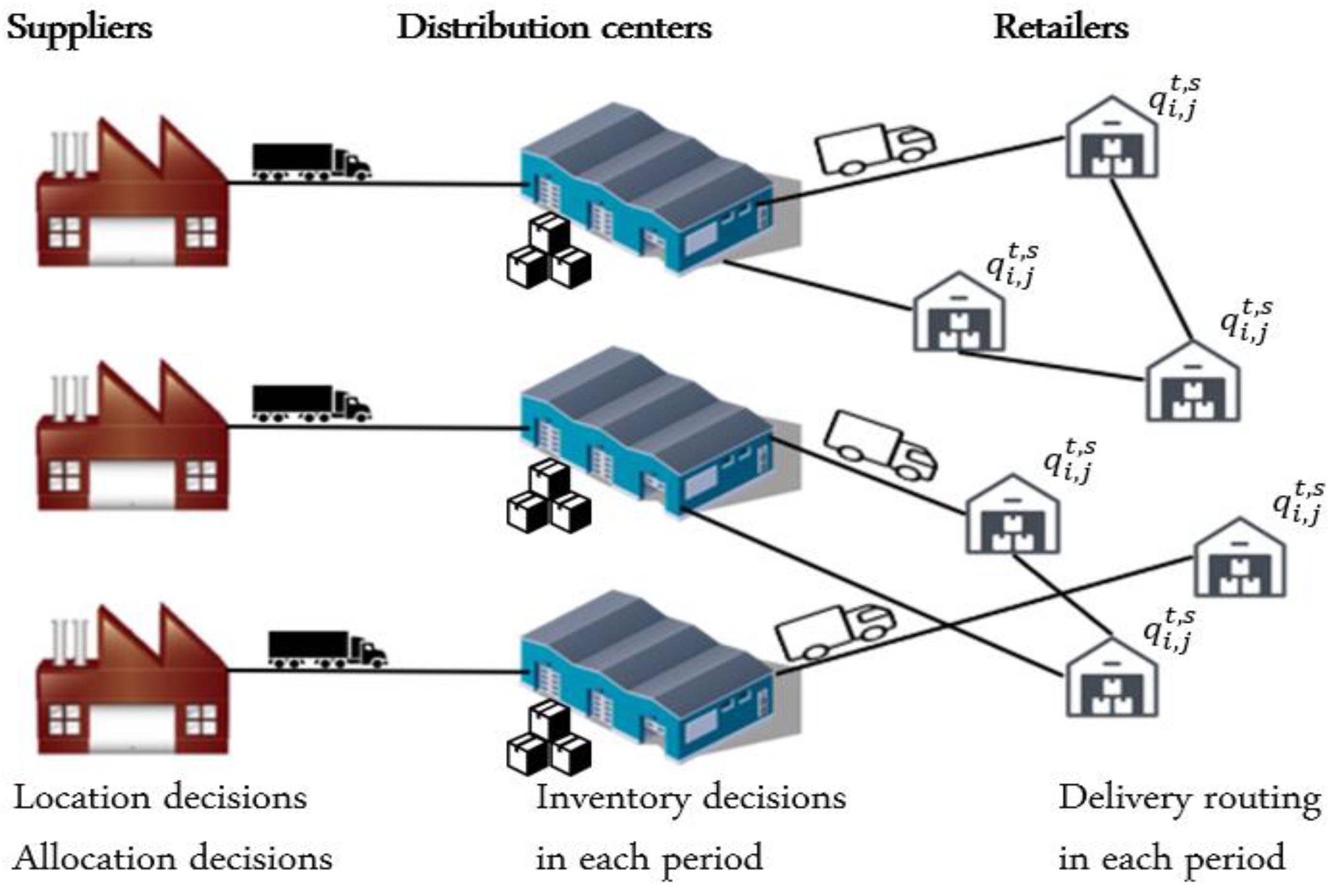
• Modelling the integrated logistics network design problem that includes routing, inventory and location–allocation decisions and considers demand fluctuations and epidemic disruptions with ripple effects.
• Applying a Monte Carlo simulation to generate plausible scenarios and model the different sources of uncertainty.
• Considering capacity augmentation and logistics collaboration as a strategy to reduce the risk of disruption.
• Assessing three aspects of sustainability and investigating the interaction between these aspects and resilience in the integrated design of two-echelon logistics networks subject to epidemic disruptions.

The remainder of this paper is organized as follows. Section 2 provides a review of the relevant works dealing with the resilient logistics network design problem. The integrated design problem under epidemic disruptions and demand uncertainty and the performance metrics are described and modelled in Section 3. Section 4 depicts the introduced solution methodology applied to deal with the studied. The computational results are presented in Section 5. Finally, Section 6 concludes this study and provides some future research directions.

2. Literature Review

This study addresses the design of resilient and sustainable logistics chains under disruptions. This section presents a state of the art of related literature in reputable databases, such as Web of Science, Scopus, ScienceDirect, Emerald, Wiley, Google Scholar and the SAGE full text collection [31]. The main keywords were supply chain design, sustainability, resilience and disruption. The data search was performed by combining the keywords.

The design of resilient supply chains subject to disruptive events has been extensively studied in recent years. Several models and decision-making approaches have also been proposed in order to solve this problem and make logistics networks leaner and globalized [32,33]. Most related studies have concentrated on facility location and allocation, considering stochastic parameters, such as demand or cost. However, few research works have considered the impact of other sources of disruptions due to multiple activity interruptions resulting from unexpected events [26]. In fact, these disruptions are unavoidable nowadays. However, those with ripple effects, such as outbreak disruptions, are more complex to manage and understand. Disruptions can be categorized into two types: isolated perturbations and cascading disruptions with ripple effects [34]. The latter are specific cases of the supply chain disruptions, as they can propagate rapidly and disperse worldwide, in contrast to isolated disruptions [35].

Operational and disruption risks with economic considerations have been discussed in several works. For instance, Klibi and Martel [36] have investigated multiple disruptions related to natural disasters and industrial accidents using a two-stage stochastic location-transport model. The authors have considered uncertainty parameters as random variables that follow a cumulative distribution function. They have also used plausible future scenario samples to simulate the disruptions. In addition, different strategies have been proposed to design resilient distribution networks. Similarly, Qin et al. [37] have addressed the logistics network design problem subject to accidental disruptions by introducing two risk mitigation strategies (fortification and inventory prepositioning in a two-stage mixed stochastic programming model). Seven different strategies applied to reconfigure the logistics networks using a linear and dynamic programming model have been discussed in [38]. Ivanov et al. [38] have used two indicators, namely, service level and sales volumes, as resilience metrics applied to assess the most resilient logistics structure. Then, Haghjoo et al. [39] have investigated the supply chain network design problem for blood supply by dealing with location–allocation decisions under disruption and facility uncertainty in a disaster situation. More recently, Kungwalsong et al. [40] have addressed the logistics network design problem considering possible disruptions at facilities. Moreover, Tolooie et al. [5] have solved a logistics network design problem under total disruption at a facility and uncertain demand.

However, as shown in the literature, the integration of decisions becomes an increasingly important issue in practice [41]. In this context, Asl-Najafi et al. [42] have incorporated inventory and location decisions to design closed-loop logistics networks under a probabilistic facility disruption risk. Likewise, Farahani et al. [43] have addressed the multiple product inventory location problem by assuming that facilities can partially fail during disruptions. The researchers have considered substitute products as a strategy to reduce the risk of disruptions in the investigated problem. Moreover, Fattahi et al. [44] have solved the logistics network design problem under operational and disruption risks with delay sensitivity. The authors have applied some mitigation and preventive resilience strategies to deal with random variation of facility capacity and demand uncertainty. Zahiri et al. [45] have discussed the hazardous materials transportation design problem under disruption risk and material perishability. In order to study uncertainties, they have developed a multi-stage stochastic mathematical model and employed two resilience strategies, namely, node criticality and network complexity. In addition, a two-stage stochastic program for a supply network design during disruption events has been introduced in [46] to optimize the location, allocation, inventory and order size decisions. The authors have proposed a new metric to assess the resilience of logistics networks, namely, the expected value of the cost increase during the recovery period when the logistics network undergoes disruption events.

In the last few years, sustainable development has become a major challenge in logistics network design problems [21,47]. In fact, green supply chain design under disruption risk has attracted the attention of the research community. For instance, Mari et al. [17] addressed the allocation and location problem in the textile industry with green objectives under facility disruption. Motivated by the advantages of integrated planning decisions, Yavari and Geraeli [48] and Yavari et al. [49] have developed a green integrated inventory-location-routing model to address the multi-period, multi-product network design problem of perishable products under power network disruption and demand uncertainty. The authors have proposed a Mixed-Integer Linear Programming (MILP) model that minimizes the expected total network cost as well as the amount of carbon emissions. In another study, Hasani et al. [50] have investigated a global logistics network under disruption, and they have presented a multi-objective optimization model in order to take into account environmental and economic aspects. The three dimensions of sustainability have been addressed in few studies in the literature. Zahiri et al. [51] have suggested a sustainable and resilient mixed integer linear programming model that incorporates location and inventory decisions under facility disruptions and fluctuating demands. In this model, uncertainty has been treated using possibilistic–stochastic programming. More recently, Mehrjerdi et al. [52] have focused, for the first time, on the interaction between sustainability and resilience in closed-loop logistics network design using two resilience strategies, namely, the multiple sourcing and information sharing strategies.

Despite the considerable impact of ripple disruptions on the overall performance of supply chains, the aforementioned studies have not examined, in depth, the types of disruptions and their ripple effects along the planning horizon. Indeed, few studies have considered epidemic disruptions with ripple effects in the design problems. In this context, Gholami-Zanjani et al. [28,53] have presented an approach to model epidemic risk for isolated and cascading disruptions in the food context. The authors have addressed the food supply network design problem by combining location and inventory decisions and optimizing the total expected cost. Moreover, they have proposed some resilience strategies by considering the economic aspect. As the risk mitigation strategies are environmentally and economically beneficial, Gholami-Zanjani et al. [30] have recently proposed an approach integrating resilience and green perspectives for food network design. Nevertheless, the authors have not assessed the social dimension of sustainability and have not taken into account the routing decisions that can deteriorate the network performance due to the ripple effects of epidemic disruptions.

Table 1. Summary of the related literature.

References	Decision Problem			Evaluated Sustainability			Disruption		Uncertain Demand
	Location	Inventory	Routing	Economic	Environmental	Social	Isolated	Ripple Effect
[36]	✓			✓			✓		✓
[37]	✓			✓			✓
[38]	✓			✓			✓
[39]	✓			✓			✓		✓
[40]	✓			✓			✓
[5]	✓			✓			✓		✓
[42]	✓	✓		✓			✓		✓
[43]	✓	✓		✓			✓
[44]	✓	✓		✓			✓		✓
[45]	✓	✓		✓					✓
[46]	✓	✓		✓			✓		✓
[17]	✓			✓	✓		✓
[48,49]	✓	✓	✓	✓	✓		✓		✓
[50]	✓	✓		✓	✓		✓		✓
[51]	✓			✓	✓	✓	✓
[52]	✓			✓	✓	✓			✓
[28,53]	✓	✓		✓			✓	✓	✓
[30]	✓	✓		✓	✓		✓	✓	✓
This study	✓	✓	✓	✓	✓	✓	✓	✓	✓

provides a classification of the related literature and allows for the input of the current paper in the literature. As Table 1 reveals, the studies reviewed so far showed several gaps in the area of a network logistics design. A clear gap is first shown in the integration of inventory, routing and location–allocation decisions in the design problem. As discussed earlier, addressing these decisions exhaustively allows companies to manage their logistics system efficiently, provide responsiveness at a lower cost and avoid generating suboptimal results [41,54,55]. Therefore, this study integrates different planning decisions and considers disruptions with ripple effects together with uncertain demand. Despite the importance of sustainability concerns and resilience in the logistics network design, the interaction of sustainability and resilience has not been sufficiently dealt with in the supply chain design literature. In this respect, this paper evaluates the performance of two resilience strategies not only from a resilience perspective, but also from a sustainability perspective in the integrated design of two-echelon logistics networks subject to epidemic disruptions.

3. Problem Definition and Mathematical Modelling

Figure 1 depicts the studied logistics network composed of two-echelon. Each supplier has a specific product and ships his goods to a distribution center in order to massify the flow, maintain inventory at the distribution center, if necessary, and then deliver these goods to retailers having uncertain demands. The latter are generated according to a known distribution. The distribution centers are usually located close to the city, while retailers are located in the urban cities. Therefore, a homogeneous fleet of semitrailer trucks are utilized to transport the goods in the first echelon, and a homogeneous fleet of small vehicles is used, in this research work, to serve retailers in the second echelon.

The objective of the considered problem is to design efficient logistics networks by determining the distribution centers to be opened, the allocation of retailers and suppliers, the inventory levels as well as the routing of shipments in each period. The locations of the distribution centers are selected from a set of candidate sites at the beginning of the planning horizon, as these decisions are strategic. This study is based on the following assumptions.

• Each retailer i can be visited once by one of the vehicles and served from a single distribution center d [54].
• Each supplier has a specific product, but all products are compatible.
• Retailers’ demand is assumed to be stochastic and follows a normal distribution [51].
• Vehicles and semitrailer trucks can conduct several routes in each period scenario [41].
• Location–allocation is a strategic decision, which is independent of the planning periods and plausible scenarios, as stated by Rafie-Majd et al. [56].
• In each distribution center, the maximum level inventory policy is applied [57]. This policy specifies that inventory quantities should only respect the maximum capacity of distribution centers, as depicted in Figure 2.

The model sets, parameters and decision variables used in the mathematical formulation are listed in

Table 2. Notations and definitions used in the mathematical modelling.

Symbol	Definition
Sets
J	Set of suppliers
D	Set of distribution centers
I	Set of retailers
A1, A2	Set of pickups and delivery routes arcs
T	Set of periods in the planning horizon
S	Set of plausible scenarios
Independent input parameters of scenarios
Capj	Maximum throughput capacity of the supplier j
Capd	Maximum throughput capacity of the distribution center d
FOd	Fixed cost of the distribution center d
ECd	Average energy consumption of the distribution center d
Qs	Semitrailer truck maximum loading capacity
Qv	Vehicle loading capacity
Fs	Operating cost of a semitrailer truck (by route)
Fv	Operating cost of a vehicle (by route)
TsE	Fuel consumption rate of an empty semitrailer truck (L/Km)
TsL	Fuel consumption rate of a fully loaded semitrailer truck (L/Km)
TvE	Fuel consumption rate of an empty vehicle (L/Km)
TvL	Fuel consumption rate of a fully loaded vehicle (L/Km)
cI	Inventory unit cost in distribution centers (€/Kg)
cp	Penalty unit cost (€/Kg)
cf	Fuel price per liter (€/L)
eF	Fuel CO2 emission factor (Kg CO2/L)
ec	CO2 emitted per energy consumption unit (Kg CO2/kwh)
Ac	Average number of accidents
di,j	Distance between two nodes i and j: $i,j\in J\cup D\cup I$
Input parameters dependent of scenarios
$q_{i,j}^{t,s}$	Demand of retailer i from supplier j in period t under scenario s
ps	Occurrence probability of scenario s, ${\sum }_{s\in S}{p}_s$ = 1
First-stage decision variables
$y_d$	Binary variable, equal to 1 if the distribution center d is open; 0, otherwise
$z_{i,d}$	Binary variable, equal to 1 if node i is assigned to center d; 0, otherwise, i ∈ I ∪ J, d ∈ D
Second-stage decision variables
$Q{1}_{j,d}^{t,s}$	Quantity delivered by supplier j to center d in period t under scenario s
$Q{2}_{j,d,i}^{t,s}$	Product quantity of supplier j delivered by center d to customer i in period t under scenario s
$I_{j,d}^{t,s}$	Inventory level of products of supplier j in center d in period t under scenario s
$x_{i,j}^{t,s}$	Binary variable, equal to 1 if arc (i; j) is traversed by a vehicle/semitrailer at period t under scenario s; 0, otherwise,
$f_{i,j}^{t,s}$	Freight quantity transported by a semitrailer truck/ vehicle on the arc (i; j) if it moves directly from node i to node j in period t under scenario s, (i; j) $\in$ A2

.

3.1. Sustainability Dimensions

The evaluation of the supply chain performance in the related literature has been mainly based on the economic indicators. In this study, we employed the three sustainability indicators introduced in [27]. We consider the different components of strategic costs and expected of tactical and operational costs. However, from an environmental point of view, the CO₂ emissions caused by transport activities and the operation of distribution centers are assessed. On the other hand, the accident rate resulting from transportation is evaluated from a social perspective.

3.1.1. Costs Calculation

The economic indicator is calculated by adding the location–allocation costs (CF) in the first stage and the expected costs of inventory (CI_s), transportation (CT_s) and penalty (CP_s) in the second stage.

The fixed costs are computed by summing the opening costs of the selected distribution centers (Equation (1)).

$$CF={\displaystyle \sum _d}{y}_{d}F{O}_d$$

(1)

The inventory cost (CI_s) under scenario s is calculated by multiplying the inventory amount in each period by the unit inventory cost using Equation (2).

$$C{I}_s={\displaystyle \sum _{t\in T}}{\displaystyle \sum _{d\in D}}{\displaystyle \sum _{j\in J}}{I}_{j,d}^{t,s}{c}_I$$

(2)

To compute the transport costs under scenario s, the formula proposed by [60] is used. In fact, as shown in Equation (3), this cost depends principally on the semitrailer truck/vehicle load and the travelled distance.

$$\begin{array}{cc}\hfill C{T}_{\mathrm{s}}=& cf[{\displaystyle \sum _{t\in T}}{\displaystyle \sum _{d\in D,j\in J}}{d}_{d,j}(T{s}_E{x}_{d,j}^{t,s}+(T{s}_L-T{s}_E)\frac{Q{1}_{j,d}^{t,s}}{Qs})\hfill \\ & +{\displaystyle \sum _{t\in T}}{\displaystyle \sum _{(i,j)\in A_2}}{d}_{i,j}(T{v}_E{x}_{i,j}^{t,s}+(T{v}_L-T{v}_E)\frac{f_{i,j}^{t,s}}{Qv})]\hfill \end{array}$$

(3)

Finally, the penalty cost CP_s under scenario s is computed by multiplying the unsatisfied demand by a unit penalty cost (Equation (4)).

$$C{P}_s=c_p{\displaystyle \sum _{t\in T}}{\displaystyle \sum _{d\in D}}{\displaystyle \sum _{j\in J}}{\displaystyle \sum _{i\in I}}{q}_{i,j}^{t,s}-Q{2}_{j,d,i}^{t,s}$$

(4)

3.1.2. Environmental Assessment

As mentioned previously, we quantify two types of CO₂ emissions, namely, emissions generated by transportation activities (ET_s) and those caused by the operation of opened distribution centers (EF). To calculate transportation emissions under scenario s, we adapt the formula introduced by Pan et al. [60]. This formula is commonly used in the literature in order to take into account the massification of flows in collaborative transport optimization [27,41,54,61,62,63]. These emissions are calculated using Equation (5).

$$\begin{array}{cc}\hfill E{T}_{\mathrm{s}}=& ef[{\displaystyle \sum _{t\in T}}{\displaystyle \sum _{d\in D,j\in J}}{d}_{d,j}(T{s}_E{x}_{d,j}^{t,s}+(T{s}_L-T{s}_E)\frac{Q{1}_{j,d}^{t,s}}{Qs})\hfill \\ & +{\displaystyle \sum _{t\in T}}{\displaystyle \sum _{(i,j)\in A_2}}{d}_{i,j}(T{v}_E{x}_{i,j}^{t,s}+(T{v}_L-T{v}_E)\frac{f_{i,j}^{t,s}}{Qv})]\hfill \end{array}$$

(5)

To estimate the emissions generated by the operation of distribution centers (EF), we utilize the same approach applied in [27,41,54] (Equation (6)).

$$EF=e_c{\displaystyle \sum _d}{y}_{d}E{C}_d$$

(6)

3.1.3. Social Sustainability Assessment

Modelling social considerations is a complex task that was not given great attention in the literature [61,64]. In this study, the social/societal impact is assessed by evaluating the accident rate caused by transportation activities, as demonstrated in [27]. The accident rate (A_s) under scenario s is calculated by applying Equation (7).

$$A_s=\frac{A_{ref}}{d_{ref}}{\displaystyle \sum _{t\in T}}{\displaystyle \sum _{(i,j)\in A_1\cup A_2}}{d}_{i,j}{x}_{d,j}^{t,s}$$

(7)

where $A_{ref}$ denotes the accident rate for a reference distance $d_{ref}$.

3.2. Measure of Resilience

In order to assess the resilience of logistics chains, we apply, in this study, a resilience metric intensively used in the literature [51,65]. This metric seeks to address the customer’s service level (%CSL) by computing the quantities transported to retailers over the total demand, as shown by Equation (8).

$$\%CSL=100\frac{{\sum }_{j\in J}{\sum }_{d\in D}{\sum }_{i\in I}{\sum }_{t\in T}{\sum }_{s\in S}Q{2}_{j,d,i}^{t,s}}{{\sum }_{i\in I}{\sum }_{j\in J}{\sum }_{t\in T}{\sum }_{s\in S}{q}_{i,j}^{t,s}}$$

(8)

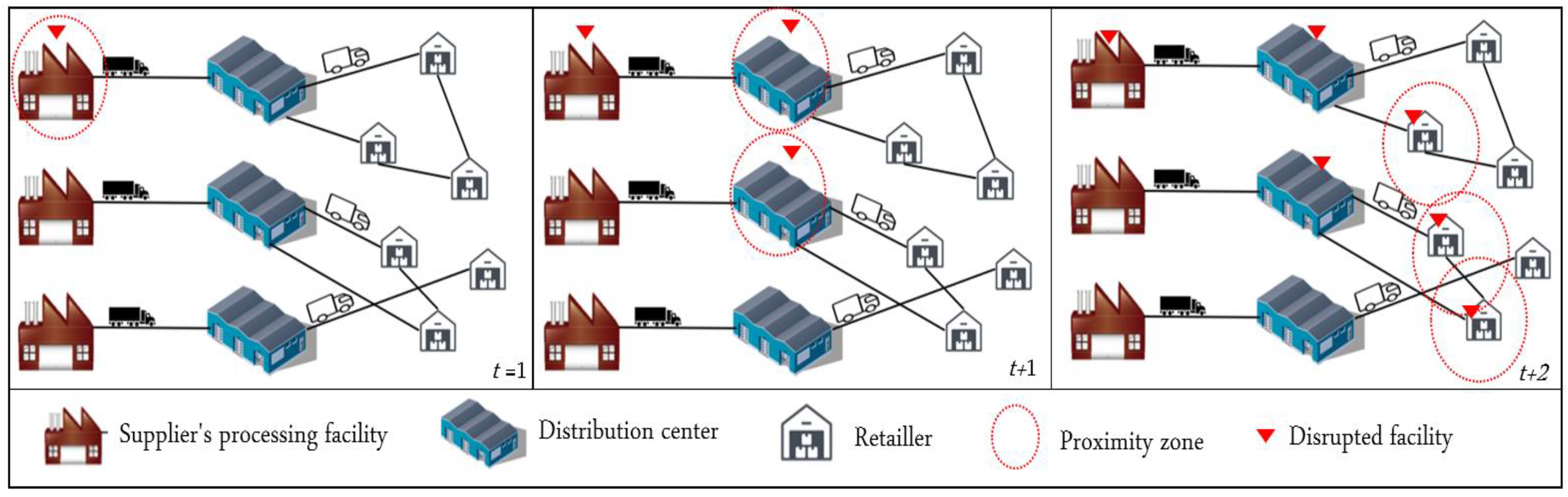
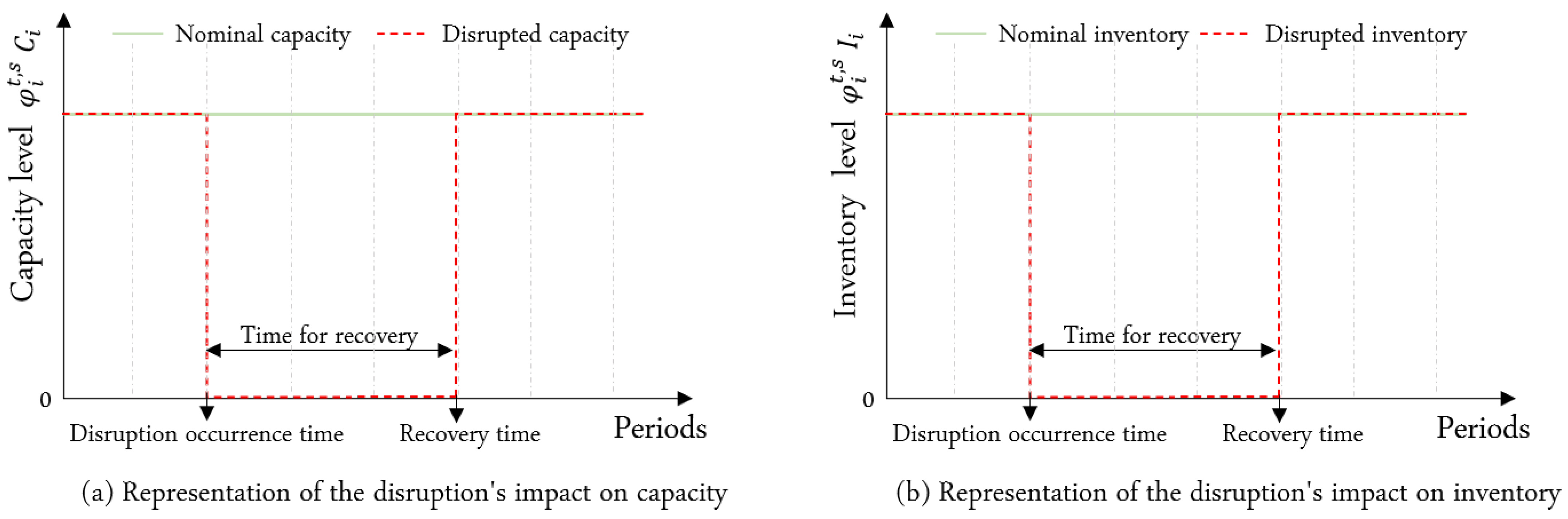
3.3. Epidemic Disruption Modelling

In this section, a simple model is presented to illustrate how cascading epidemic disruptions with ripple effects can arise, damage facilities and propagate to the neighboring ones. These disruptions are principally characterized by their intensity (low frequency/high impact), recovery time and rapid spreading in the network [30]. Figure 3 depicts the schematic representation of the ripple effects in a multi-period two-echelon logistics network, as revealed in [53].

As shown in Figure 3, when an epidemic disruption arrives at time t, a primary facility is affected, and the other platforms directly or indirectly connected to that primary facility are exposed to the risk of propagation. Moreover, depending on the correlations and interactions between facilities, the propagation of the disruption may spread to the next periods (t + 1, t + 2, …), which become themselves infected nodes, and so on, resulting in the ripple effects. To do this, a correlation matrix is used for propagation probabilities, where values are based mainly on regional proximity and flow relationships.

The modeling approach is based on a probabilistic approach revealing how cascading epidemic disruptions with ripple effects may arise in unpredictable ways over the planning horizon. The disruption model includes essentially two steps. The first one consists in simulating the characteristics of disruption, namely, disruption arrival time. However, the second step aims at simulating the response times and testing the propagation effect on facilities, in terms of capacity and inventory losses. As previously discussed in the literature [36,38,53], epidemic disruptions are described by two correlated factors, namely, the intensity of the impact and the recovery time. In fact, when an outbreak disruption occurs in a zone or in a specific facility, the throughput capacity and the inventory level drop to zero since the facility is closed and the inventory is eliminated. Then, they are fully recovered after the recovery time. This impact can be defined by a discrete recovery function, as exposed in Figure 4.

In order to simulate the arrival and recovery time as well as the spread of disruption, a Monte Carlo simulation procedure was used in the conducted experiment. The goal of this procedure is to stochastically generate the loss parameter ${\phi }_i^{t,s}$ corresponding to the lost part of the nominal capacity and the stock level, which is generally between 0 and 1. This stochastic parameter is utilized to formulate the mathematical model.

3.4. Stochastic Mathematical Model

In this section, a stochastic Two-Stage Mixed-Integer Linear Program (2S-MILP) with a stochastic demand and random epidemic perturbation is developed. In the 2S-MILP, the stochastic parameters are considered as random variables with an associated probability distribution. Moreover, the proposed model involves a two-stage decision making process. The first stage consists in determining the number of distribution centers, the optimal location of facilities and the allocation of suppliers and retailers that are independent of the disruption scenarios. However, decisions on the inventory level, the routes and the supplied quantities (operational variables include an index s that designates the particular realization of the scenario) are determined in the second stage based on facilities location–allocation and the realized uncertainty in each scenario. The total objective function in the proposed model is obtained by summing the objective values of the first stage and the expected values of all scenarios in the second stage. The problem is formulated mathematically as follows:

$$E(CT)=min{\displaystyle \sum _d}{\displaystyle \sum _t}{y}_{d}F{O}_d+{\displaystyle \sum _{s\in S}}{p}_{s}Q(X,s)$$

(9)

where X denotes the vector of all the design variables used in the second stage, p_s is the occurrence probability of scenario s and $Q(X,s)$ is the optimal objective value of the second-stage problem in scenario s.

$$Q(X,s)=C{I}_s+C{T}_{\mathrm{s}}+C{P}_{\mathrm{s}}$$

Subject to constraints:

$$z_{i,d}\le y_d\forall d\in D,\forall i\in I\cup J$$

(10)

$${\displaystyle \sum _{j\in J}}{z}_{j,d}=1\forall d\in D$$

(11)

$${\displaystyle \sum _{d\in D}}{z}_{i,d}\le 1\forall i\in I\cup J$$

(12)

$$I_{j,d}^{0,s}=0\forall j\in J,\forall d\in D,\forall s\in S$$

(13)

$$I_{j,d}^{t,s}=(1-{\phi }_d^{t,s})(Q{1}_{j,d}^{t,s}+I_{j,d}^{t-1,s})-{\displaystyle \sum _{iϵI}}Q{2}_{j,d}^{1,s}\forall d\in D,\forall t\in T,\forall j\in J,\forall s\in S$$

(14)

$$I_{j,d}^{t,s}\le (1-{\phi }_d^{t,s})ca{p}_d{y}_d\forall d\in D,\forall t\in T,\forall j\in J,\forall s\in S$$

(15)

$${\displaystyle \sum _{j\in J}}Q{1}_{j,d}^{t,s}\le (1-{\phi }_d^{t,s})ca{p}_d{y}_d-{\displaystyle \sum _{j\in J}}{I}_{j,d}^{t-1,s}\forall t\in T,\forall d\in D,\forall s\in S$$

(16)

$$Q{1}_{j,d}^{t,s}\le (1-{\phi }_j^{t,s})ca{p}_j{x}_{d,j}^{t,s}\forall d\in D,\forall j\in J,\forall t\in T,\forall s\in S$$

(17)

$${\displaystyle \sum _{i\in J\cup I}}{z}_{i,d}{q}_{i,j}^{t,s}\le (1-{\phi }_d^{t,s})ca{p}_d{y}_d\forall d\in D,\forall tϵT,\forall sϵS$$

(18)

$$Q{2}_{j,d,i}^{t,s}\le (1-{\phi }_d^{t,s})ca{p}_d{z}_{i,d}\forall t\in T,\forall i\in I,j\in J\cup D,\forall s\in S$$

(19)

$${\displaystyle \sum _{jϵJ}}{\displaystyle \sum _{dϵD}}Q{2}_{j,d,i}^{t,s}\le (1-{\phi }_i^{t,s}){\displaystyle \sum _{jϵJ}}{q}_{i,j}^{t,s}\forall j\in J,\forall i\in I,\forall d\in D,\forall t\in T,\forall s\in S$$

(20)

$$Q{1}_{j,d}^{t,s}\le Qs{x}_{d,j}^{t,s}\forall i\in I,\forall t\in T,\forall s\in S$$

(21)

$$x_{d,j}^{t,s}\le z_{j,d}\forall t\in T,\forall j\in J,\forall s\in S,\forall d\in D$$

(22)

$$x_{d,j}^{t,s}=x_{j,d}^{t,s}\forall t\in T,\forall j\in J,\forall s\in S,\forall d\in D$$

(23)

$${\displaystyle \sum _{i\in I\cup D}}{x}_{i,j}^{t,s}\le 1\forall t\in T,\forall i\in I,\forall s\in S$$

(24)

$${\displaystyle \sum _{i\in I}}{x}_{d,i}^{t,s}={\displaystyle \sum _{i\in I}}{x}_{i,d}^{t,s}\forall t\in T,\forall d\in D,\forall s\in S$$

(25)

$${\displaystyle \sum _{i\in I\cup D}}{x}_{j,i}^{t,s}={\displaystyle \sum _{i\in I\cup D}}{x}_{i,j}^{t,s}\forall t\in T,\forall d\in D,\forall s\in S$$

(26)

$$x_{d,i}^{t,s}\le z_{i,d}\forall t\in T,i\in I,\forall d\in D,\forall s\in S$$

(27)

$$x_{i,d}^{t,s}\le z_{i,d}\forall t\in T,i\in I,\forall d\in D,\forall s\in S$$

(28)

$$x_{i,i’}^{t,s}+z_{i,d}+z_{i’,d’}\le 2\forall t\in T,i,i’\in D,\forall d,d’\in D,\forall s\in S$$

(29)

$${\displaystyle \sum _{j\in I\cup D}}{f}_{j,i}^{t,s}-{\displaystyle \sum _{j\in I\cup D}}{f}_{i,j}^{t,s}={\displaystyle \sum _{d\in D}}{\displaystyle \sum _{j\in J}}Q{2}_{j,d,i}^{t,s}\forall t\in T,\forall i\in I,\forall s\in S$$

(30)

$$f_{i,j}^{t,s}\le Q_v{x}_{i,j}^{t,s}\forall t\in T,\forall i,j\in I\cup D,\forall s\in S$$

(31)

$${\displaystyle \sum _{i\in I}}{f}_{i,d}^{t,s}\le 0\forall t\in T,\forall i,j\in J\cup D,\forall s\in S$$

(32)

$$z_{i,d},y_d\in \left\{0,1\right\}\forall d\in D,\forall i\in I\cup J$$

(33)

$$x_{i,j}^{t,s}\in \left\{0,1\right\}\forall t\in T,\forall (i,j)\in A1\cup A2,\forall s\in S$$

(34)

$$Q{1}_{j,d}^{t,s},Q{2}_{j,d,i}^{t,s},I_{j,d}^{t,s}\ge 0\forall t\in T,\forall i\in I,\forall j\in J,\forall d\in D,\forall s\in S$$

(35)

$${\mathrm{f}}_{\mathrm{i},\mathrm{j}}^{\mathrm{t},\mathrm{s}}\ge 0\forall t\in T,\forall (i,j)\in A2,\forall s\in S$$

(36)

The objective function E(CT) (9) minimizes the network total expected cost, including the first-stage costs (the strategic costs related to the opening of the distribution centers) and the expected second-stage costs related to the inventory levels, transportation and unmet demand. Constraints (10), (11) and (12) concern the first-stage decisions, i.e., allocation decisions. Constraint (10) ensures that customers and suppliers can only be assigned to one distribution center that is open over the planning horizon. Constraint (11) ensures that each supplier must be assigned to one distribution center. Constraint (12) guarantees that each retailer must be assigned to no more than one distribution center. Constraints (13), (14), (15) and (16) define the inventory levels at the distribution centers in the second stage. More precisely, constraint (13) describes the initial inventory level of each distribution center in each scenario $s\in S$. Constraint (14) determines the inventory levels in the distribution centers at each period t under scenario $s\in S$. Constraint (15) ensures that the inventory level in each distribution center cannot exceed the available storage capacity in each scenario s. Constraint (16) expresses that the amount of goods to be delivered to the distribution center d will never exceed its capacity for each planning period in each scenario s. Constraint (17) guarantees that the quantity sent by a supplier must not exceed the maximum capacity throughput of its facility in period t under scenario s. Constraint (18) ensures that customers and suppliers are assigned to distribution centers and that the capacities of the latter are satisfied in all period planning and under possible scenario s. Constraint (19) guarantees that the goods distributed by each distribution center must not exceed its maximum capacity. Constraint (20) ensures that the quantities transported to retailers should not exceed their demands. Constraint (21) ensures that the quantity loaded on the semitrailer truck must not exceed its capacity on the arc (d, j) under scenario s. Constraint (22) requires that the arc (d, j) is traversed if only the supplier j is assigned to center d. Constraint (23) guarantees an equal number of incoming and outgoing arcs in the first echelon. Constraints (24)–(32) guarantee a reasonable delivery process in the second echelon under each scenario s. Constraint (24) ensures that each retailer is visited at most once in each planning period. Constraints (25) and (26) guarantee an equal number of incoming and outgoing arcs in the second echelon. Constraints (27), (28) and (29) eliminate unauthorized routes that do not start and finish at the same distribution center. Constraint (30) ensures the flow conservation for the collection process. Constraint (31) ensures that vehicle capacities are not violated. Constraint (32) imposes that the quantities returned to the distribution centers must be zero. Finally, Constraints (33)–(36) specify the nature of each decision variable used in this modelling.

3.5. Resiliency and Sustainability Strategies Formulations

In this section, two resilience strategies are formulated and added to the disrupted model to attenuate the effects of disruption on the sustainable performance of a logistic network, namely, capacity expansion and logistics collaboration as one proactive resilience strategy.

3.5.1. Capacity Expansion

The first resiliency strategy introduced in the basic model is the capacity expansion strategy for facilities. In fact, logistics facilities can increase their capacity temporarily in order to face disruptions through an available capacity reserve. In this respect, the variables $cap{F}_j^{t,s}$, $cap{C}_d^{t,s}$ and $cap{R}_i^{t,s}$ are defined to determine the amount of the extended capacity in each period for suppliers, distribution centers and retailers, respectively. For this, we modify constraints (15)–(20) in the basic model by the following constraints, (37)–(42).

$$I_{j,d}^{t,s}\le (1-{\phi }_d^{t,s})ca{p}_d{y}_d+cap{C}_d^{t,s}\forall d\in D,\forall t\in T,\forall j\in J,\forall s\in S$$

(37)

$${\displaystyle \sum _{j\in J}}Q{1}_{j,d}^{t,s}\le (1-{\phi }_d^{t,s})ca{p}_d{y}_d-{\displaystyle \sum _{j\in J}}{I}_{j,d}^{t-1,s}+cap{C}_d^{t,s}\forall t\in T,\forall d\in D,\forall s\in S$$

(38)

$$Q{1}_{j,d}^{t,s}\le (1-{\phi }_j^{t,s})ca{p}_j{x}_{d,j}^{t,s}+cap{F}_j^{t,s}\forall d\in D,\forall j\in J,\forall t\in T,\forall s\in S$$

(39)

$${\displaystyle \sum _{i\in J\cup I}}{z}_{i,d}{q}_{i,j}^{t,s}\le (1-{\phi }_d^{t,s})ca{p}_d{y}_d+cap{C}_d^{t,s}\forall d\in D,\forall t\in T,\forall s\in S$$

(40)

$$Q{2}_{j,d,i}^{t,s}\le (1-{\phi }_d^{t,s})ca{p}_d{z}_{i,d}+cap{C}_d^{t,s}\forall t\in T,\forall i\in I,j\in J\cup D,\forall s\in S$$

(41)

$${\displaystyle \sum _{jϵJ}}{\displaystyle \sum _{dϵD}}Q{2}_{j,d,i}^{t,s}\le (1-{\phi }_i^{t,s}){\displaystyle \sum _{jϵJ}}{q}_{i,j}^{t,s}+cap{R}_i^{t,s}\forall j\in J,\forall i\in I,\forall d\in D,\forall t\in T,\forall s\in S$$

(42)

This strategy generates an additional cost by reserving a specific location for this tampon in the facility and the operational cost associated with this capacity expansion. Therefore, $C{S}_j^{t,s}$, $C{S}_d^{t,s}$ and $C{S}_I^{t,s}$ are defined as unit capacity expansion costs expressed by the Equation (43) in the objective function.

$${\displaystyle \sum _{jϵJ}}{\displaystyle \sum _{tϵT,sϵS}}cap{F}_j^{t,s}C{S}_j^{t,s}+{\displaystyle \sum _{dϵD}}{\displaystyle \sum _{tϵT,sϵS}}cap{C}_d^{t,s}C{S}_d^{t,s}+{\displaystyle \sum _{iϵI}}{\displaystyle \sum _{tϵT,sϵS}}cap{R}_i^{t,s}C{S}_i^{t,s}$$

(43)

Similarly, the temporary expansion of capacities causes additional emissions due to the operations made by facilities. Consequently, ECE is defined as capacity expansion unit emissions expressed by the Equation (44) in the emissions estimation.

$${\displaystyle \sum _{jϵJ}}{\displaystyle \sum _{tϵT,sϵS}}cap{F}_j^{t,s}ECE{e}_c+{\displaystyle \sum _{dϵD}}{\displaystyle \sum _{tϵT,sϵS}}cap{C}_d^{t,s}ECE{e}_c+{\displaystyle \sum _{iϵI}}{\displaystyle \sum _{tϵT,sϵS}}cap{R}_i^{t,s}ECE{e}_c$$

(44)

3.5.2. Logistics Collaboration

The integration of the logistics collaboration strategy between suppliers has become a strategic challenge for companies who seek to achieve their economic, social and environmental sustainability objectives [21]. In the context of the shared management of resources and means, this strategy has also become more promising by sharing information related to the evolution and diffusion of the existing disruptions. Therefore, we remove the unicity assignment constraints (11) and define a new decision variable ($f_{i,j}^{t,s}(i,j)\in A1$) to model product collection in the first rung. The following constraints (45)–(52) are added in the perturbed model to incorporate this strategy:

$${\displaystyle \sum _{i\in J\cup D}}{x}_{i,j}^{t,s}\le 1\forall t\in T,\forall j\in J,\forall s\in S$$

(45)

$${\displaystyle \sum _{j\in J}}{x}_{d,j}^{t,s}={\displaystyle \sum _{j\in J}}{x}_{j,d}^{t,s}\forall t\in T,\forall d\in D,\forall s\in S$$

(46)

$${\displaystyle \sum _{i\in J\cup D}}{x}_{i,j}^{t,s}={\displaystyle \sum _{i\in J\cup D}}{x}_{j,i}^{t,s}\forall t\in T,\forall j\in J,\forall s\in S$$

(47)

$$x_{j,d}^{t,s}\le z_{j,d}\forall t\in T,j\in J,\forall d\in D,\forall s\in S$$

(48)

$$x_{j,j’}^{t,s}+z_{j,d}+z_{j’,d’}\le 2\forall t\in T,j,j’\in D,\forall d,d’\in D,\forall s\in S$$

(49)

$${\displaystyle \sum _{i\in J\cup D}}{f}_{j,i}^{t,s}-{\displaystyle \sum _{i\in J\cup D}}{f}_{i,j}^{t,s}={\displaystyle \sum _{d\in D}}Q{1}_{j,d}^{t,s}\forall t\in T,\forall j\in J,\forall s\in S$$

(50)

$$f_{j,i}^{t,s}\le Q_s{x}_{i,j}^{t,s}\forall t\in T,\forall i,j\in J\cup D,\forall s\in S$$

(51)

$${\displaystyle \sum _{j\in J}}{f}_{d,j}^{t,s}\le 0\forall t\in T,\forall i,j\in J\cup D,\forall s\in S$$

(52)

4. Solution Methodology

This section presents the solution approach used to solve the proposed model and the different design configurations introduced in this study.

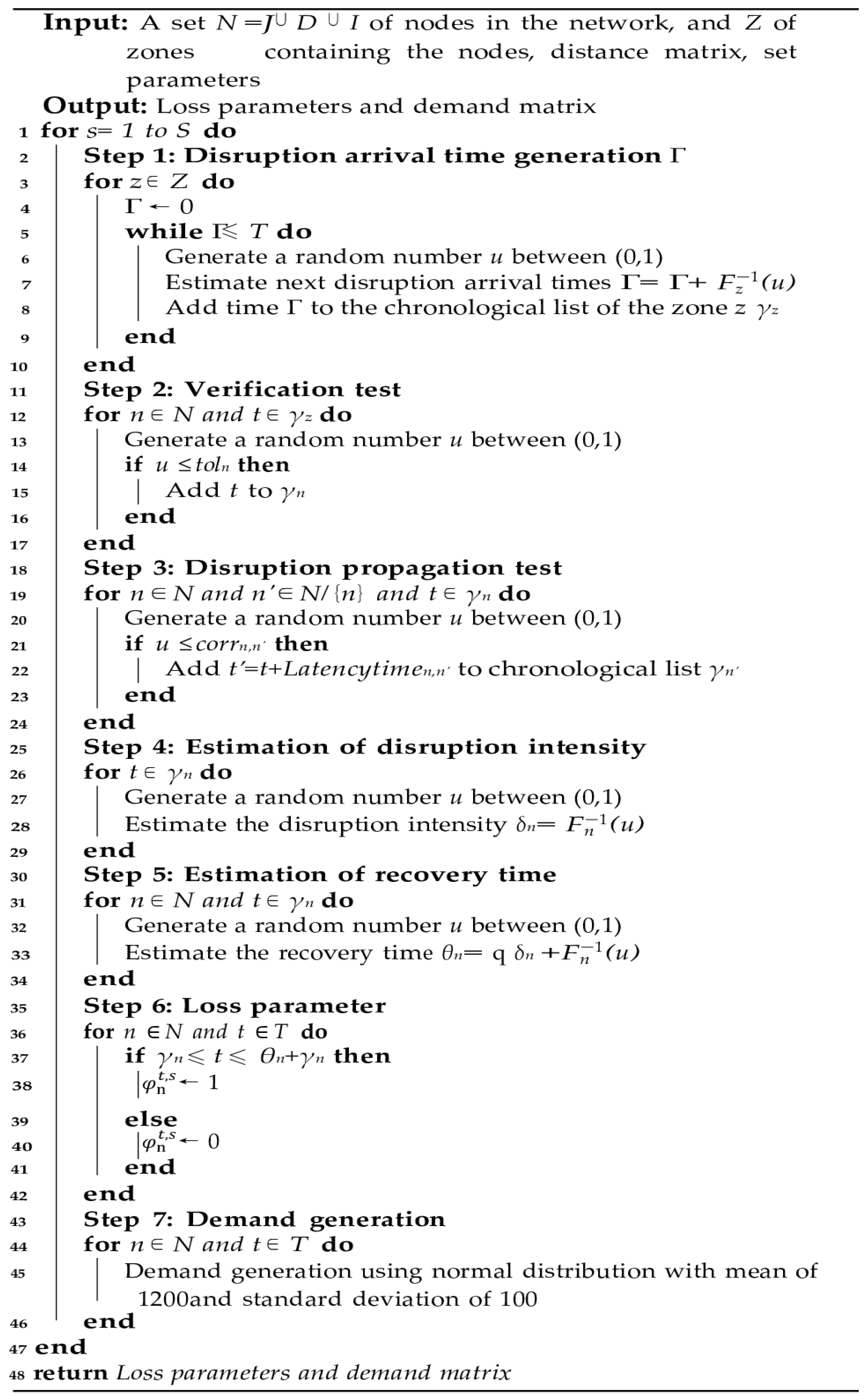
4.1. Scenarios Generation by a Monte Carlo Simulation

To address the different characteristics of the previously mentioned disruptions, we apply a probabilistic modelling approach to estimate the occurrence of these disruptions, their impact on facilities as well as their propagation in time and space over the logistics network. This approach is based on the risk modelling framework introduced by Klibi et al. [66] and Gholami-Zanjani et al. [53]. It also relies on a Monte Carlo simulation applied to generate plausible future scenarios based on statistical information of uncertain parameters. The used Monte Carlo simulation procedure is depicted in Figure 5. over the planning periods and for each scenario according to a normal distribution.

As demonstrated in the latter, the scenario generation procedure is composed of seven main steps. In the first step, the disruption arrival time for each zone is randomly generated according to the exponential distribution. Then, a chronological list of disruption occurrence times for each zone is formed. In the second step, a verification test for each node located in the disrupted zone is performed to show if the node is disrupted or not. Subsequently, a chronological list of disruption occurrence times is constructed for each node in the network. In the third step, a propagation test of the disruption is carried out. To do this, a correlation matrix, based on the material flow and the distance between the nodes, is used. Afterwards, the chronological list of disruption times for each node is updated. In the fourth step, a disturbance intensity is randomly generated for each disturbance time. Fifth, the intensity estimated in step 4 is used to determine the recovery time required for each facility to return to normal operations. The linear relationship between these two parameters was studied in [66]. In step 6, the disruption impact is calculated as a loss parameter based on the previous steps. Finally, the demands are generated independently

4.2. Sample Average Approximation Method

The Monte Carlo sampling technique is applied to construct a smaller sample average problem instead of solving the problem with all possible scenarios [40]. This approach is known as the Sample Average Approximation (SAA) method. The latter has been widely used in the last few years to make near-optimal approximations of stochastic problems [30]. In fact, the SAA method approximates the stochastic model by a deterministic equivalent model, based on the Monte Carlo scenario sampling method. This technique, relying on the repetition of the sampling method M times, considers N scenarios generated in the sample as equiprobable. In this study, the SAA method is applied and the basic model is approximated as follows:

$$min{\displaystyle \sum _d}{\displaystyle \sum _t}{y}_{d}F{O}_d+\frac{1}{N}{\displaystyle \sum _{s\in S^N}}Q(X,s)$$

(53)

subject to Constraints (10)–(53), $\forall s\in S$.

5. Computational Experiments

In order to test the proposed model and the different variants that incorporate resilience and sustainability strategies, we tested the models on two instance problems. All performed experiments were solved with CPLEX 12.9.0 in a PC running Windows 10 Home 64-bit with an Intel Core i5-10210U@ 1.6 GHz and 16 GB RAM. In this section, the used data are first described. Then, the computational results are illustrated.

5.1. Description and Data

Two instances of logistics networks, with different numbers of suppliers, distribution centers and customers, were investigated in this study, as shown in

Table 3. Size of the tested problems.

Instance	Number of Suppliers	Number of Distribution Centers	Number of Retailers	Number of Periods	Number of Replications	Number of Scenarios
I1	2	2	5	12	5	10
I2	3	3	9	12	5	10

. The first test problem was randomly generated, while the second was inspired from a case study conducted in France [54]. The planning horizon considered for each problem was 12 periods. Each planning period was equal to one month. In the experiments, 50 scenarios were generated using the Monte Carlo procedure. Then, they were classified into 5 replication groups to apply the SAA approach five times (M = 5). More precisely, for each replication, 10 plausible scenarios were considered. The other parameters used in the computational experiments were extracted from the literature and are listed in

Table 4. Values of the input parameters used in the numerical experiments along with the relevant data sources.

Parameter	Value/Estimation	Source
Capj	20,000 Kg	Assumption
Capd	20,000 Kg	Assumption
FOd	6000 €	[67]
ECd	10,000 Kwh	[68]
Qs	20,000 Kg	[69]
Qv	10,000 Kg	[69]
Fs	300 €	[69]
Fv	200 €	[69]
TsE	0.15 L/km	[70]
TsL	0.31 L/km	[70]
TvE	0.13 L/km	[70]
TvL	0.15 L/km	[70]
cI	0.01 €/Kg	[59]
cp	1.5 €/Kg	Assumption
cf	1.5 €/L	[27,41]
eF	2.66 Kg CO2/L	[71]
ec	0.087 Kg CO2/L	[68]
Ac	2768 accidents per year	[54]

[27,41].

5.2. Results and Discussion

To assess the performance of the introduced strategies in designing sustainable and resilient logistics networks, we report and discuss, in this section, the findings obtained in five design configurations, namely, the non-disrupted model (NDM), the disrupted model (DM), the disrupted model with the capacity expansion strategy (DMCE), the disrupted model with a logistics collaboration strategy (DMCL) and the disrupted model with both capacity expansion and logistics collaboration strategy (DMCECL). These configurations were evaluated against five key performance indicators. The obtained results are presented in

Table 5. Comparison of the design configurations with five performance indicators.

Instance	Configuration	Expected Cost (€)	Expected Emissions (Kg CO2)	Expected Accident Rate (%)	Average Number of Opened DCs	Service Level (%)
I1	NDM	21,067.019	3491.360	21.050	2	100.00
	DM	47,765.679	3300.762	18.211	2	73.38
	DMCE	29,517.612	4100.046	25.724	2	99.66
	DMCL	38,742.400	2207.619	15.368	1	73.96
	DMCECL	19,113.490	2797.541	20.576	1	99.87
I2	NDM	31,858.988	6663.545	50.831	3	100.00
	DM	73,897.477	6626.066	51.055	3	77.53
	DMCE	46,672.017	8115.822	54.675	3	98.75
	DMCL	58,248.953	3526.752	30.153	1	77.48
	DMCECL	30,891.362	3902.640	35.679	1	99.54

.

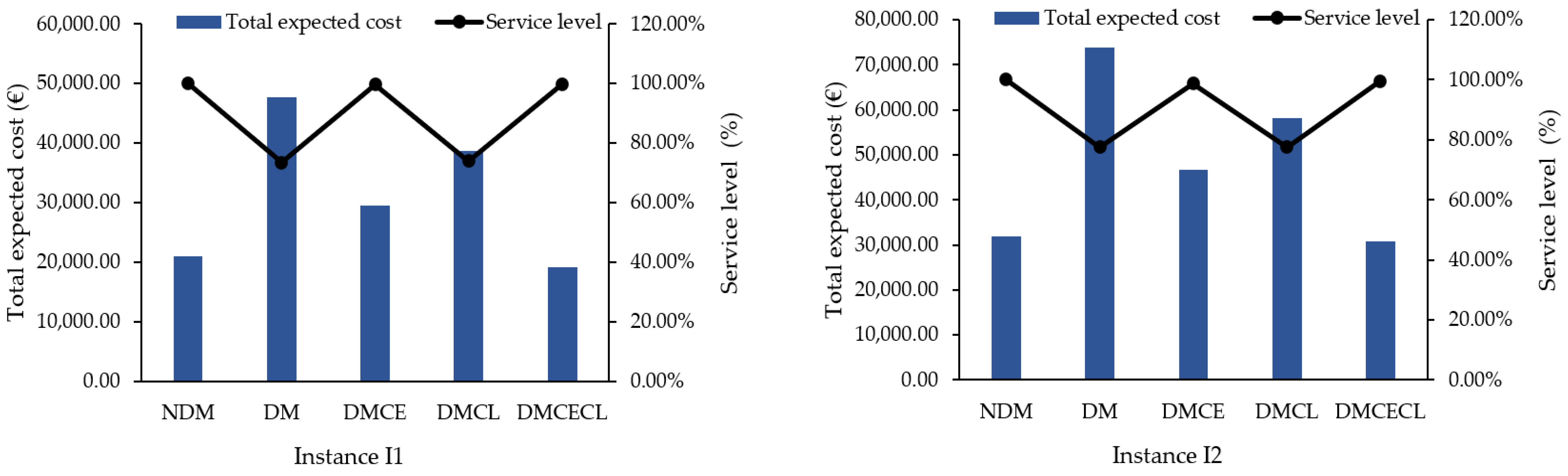
5.2.1. Economic Resilience Performance Analysis

The first analysis was conducted to assess the economic dimension and the resilience matrix of each logistics configuration. Figure 6 shows the results obtained in the five considered design configurations in terms of cost and level of service.

As represented in Figure 5 and Table 5, the different considered configurations provided different costs and service levels. In fact, the NDM configuration led to the highest service level, compared to the other configurations, especially the DM and DMCL design configurations. Obviously, since disruptions were not considered in the NDM model, the NDM configuration had the lowest logistics costs, in comparison to the DM, DMCE and DMCL configurations. However, by incorporating epidemic disruptions and demand uncertainty into the design models, the DM configuration, as a self-resilient design model, was characterized by very high costs and low service levels. This result can be explained by the considerable impact of these disruptions on facility capacities and inventory levels, which can result in higher penalty costs due to unmet demands. Furthermore, it is clear that the DMCE model, as a design model with a reactive resiliency strategy, had the highest level of service, compared to the DM and DMCL configurations. Since capacity expansion incurs additional costs, the DMCE design had higher costs than the NDM configuration. In addition, as capacity expansion improves customer satisfaction, the expected penalty costs and total cost were lower than the DM design. Additionally, as shown in Table 5, the DMCL configuration with a collaborative strategy could reduce the number of opened distribution centers, which minimizes the fixed facility costs. Obviously, logistics collaboration can improve the resiliency level and decrease the total costs by sharing non-disrupted facilities in the network.

Finally, it can be noticed that the DMCECL configuration outperformed the other design configurations under disruption in terms of cost and resilience level. The DMCECL configuration that incorporates two resilience strategies provided almost similar results to those produced by the non-disrupted configuration NDM.

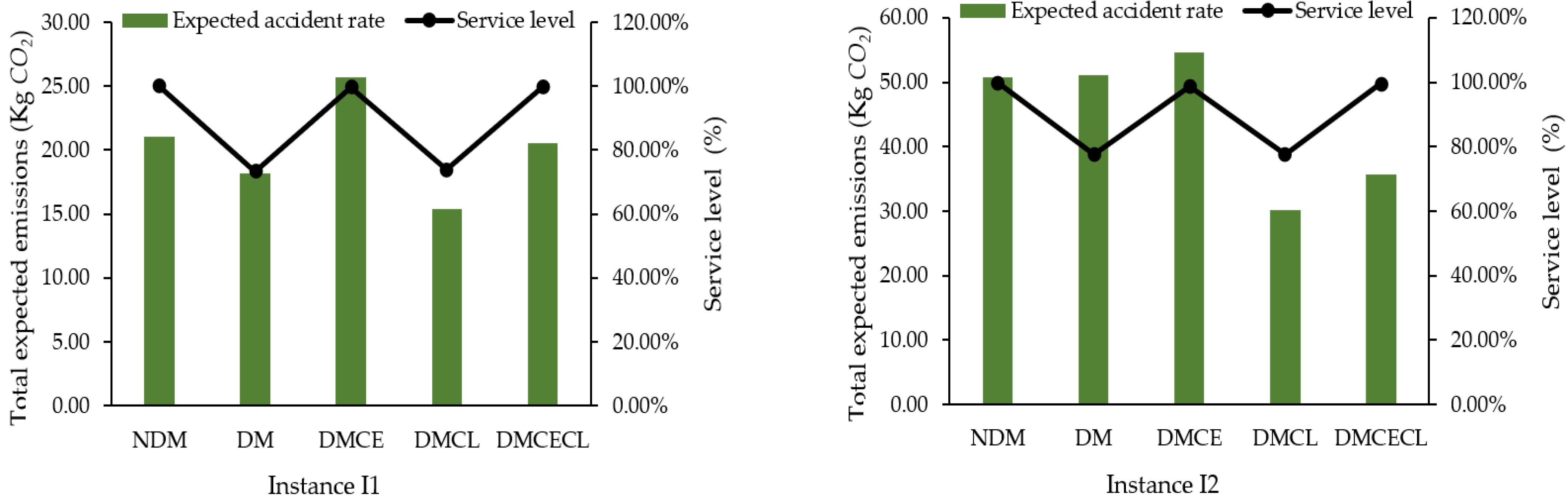
5.2.2. Environmental Resilience Performance Analysis

Figure 7 illustrates the results of the a posteriori evaluation of emissions and service levels for the different design models.

These findings reveal that the DMCE configuration considerably augmented CO₂ emissions compared to the other design models, due to the temporary capacity increase that allowed mitigating the loss of service levels. Moreover, as can be seen in Figure 7, the DM configuration generated slightly lower quantities of CO₂ emissions than the unperturbed NDM model, due to the fact that the integration of disturbances in the model can reduce the satisfaction rate and, consequently, minimize the number of trips for products transportation. In addition, it is obvious that the collaborative strategy in the disrupted model resulted in a significant reduction of transportation and facility operations emissions by slightly increasing the service rate obtained by the disrupted model with free resilience. Moreover, the integration of capacity expansion and logistics collaboration strategies can offer a good trade-off between the resilience and emissions levels in the disrupted logistics networks.

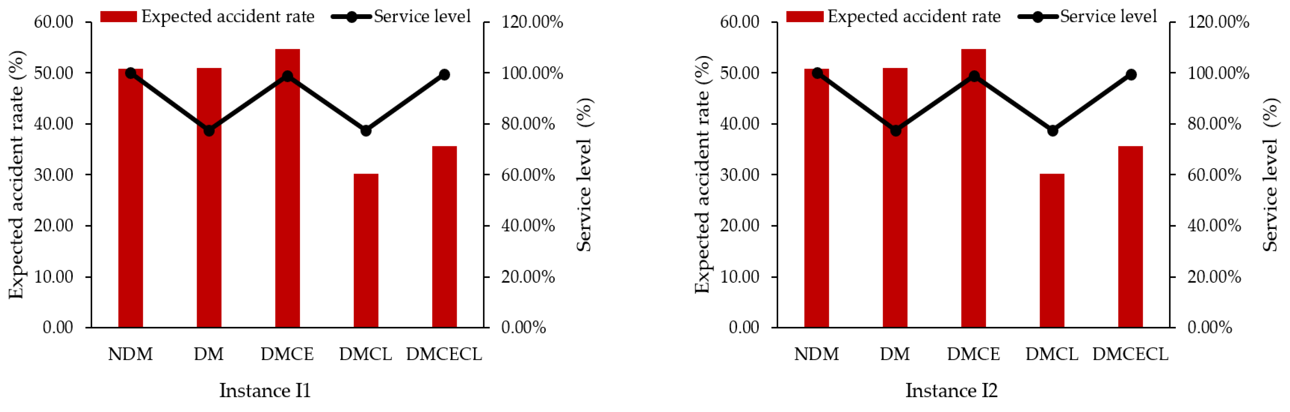
5.2.3. Social Resilience Performance Analysis

The expected accident rate and service levels obtained in each configuration are compared in Figure 8. The results demonstrated that the DMCE configuration provided a more significant accident rate compared to the other configurations, due to the increase in the number of empty and loaded trips in order to improve the satisfaction rate. Moreover, it can be observed that, when disruptions were not integrated, the accident rates were higher than those obtained by the DMCL and DMCECL configurations. However, from a resiliency point of view, we can conclude that the DMCECL configuration provided almost the same service level as the non-disrupted one.

The illustrative examples demonstrate that, with the integration of capacity augmentation and logistics collaboration strategies, the effects of disruptions can be avoided and the logistics operations sustainability can be improved.

5.3. Managerial Implications

In recent years, the growing concerns about disruption risks and sustainability challenges have led companies to explore high-performance strategies to remain competitive and ensure their global performance. In addition, integrated planning decisions have become key issues in logistics network management. Despite the numerous intersections and relationships between resilience, sustainability and planning decisions, the literature on resilient and sustainable integrated logistics network planning remains scarce. Accordingly, the sustainability and resilience assessment of a two-echelon integrated logistics network design is investigated in the present paper. This study can guide logistics decision-makers and managers to face the epidemic disruption risks and ensure the sustainability of their logistics operations. Indeed, it helps managers obtain insights to select the most powerful resilience and sustainability strategies in order to mitigate vulnerabilities in logistics networks. The numerical results prove that the integration of two strategies, namely, capacity expansion and logistics collaboration, leads to high resilience and sustainability levels. Indeed, this combination does not only increase the service level in disrupted logistics networks, but also reduces costs, CO₂ emissions and the accident rate due to transport activities.

6. Conclusions

Logistics network resiliency and sustainability has become more vital to create a competitive business environment. This study proposed a comprehensive stochastic model for a two-echelon logistics network design under epidemic disruptions and demand uncertainty. To mitigate the risk of disruptions and improve the sustainability of logistics networks, two design strategies were integrated into the mathematical model. Then, a Monte Carlo sampling technique was used to make near-optimal approximation of the scenario-based stochastic model. Scenarios were generated using a Monte Carlo procedure. Applying the introduced strategies, different design models were obtained. These models were tested with plausible scenarios and under two instance problems. The results revealed that different design patterns have distinct behaviors and implementing two strategies together could significantly increase the performance of the network. More precisely, the integration of logistics collaboration and capacity expansion can significantly reduce logistics costs, CO₂ emissions and accident risk resulting from transportation while ensuring a very high level of network resiliency.

Several research perspectives can be recommended to enrich this promising topic. Firstly, large-sized instances require high computation times to find the optimal solution. Therefore, it is important to propose heuristics to solve models with large-scale problems [72]. Secondly, the two objectives of environmental and social sustainability were evaluated a posteriori for each logistics configuration. Consequently, addressing sustainability objectives in conjunction with resilience considerations may offer more comprehensive decision support for decision-makers [30]. Furthermore, considering both forward and reverse flows in the supply chain and perishability of products could be another advocated issue for future research. Fourth, considering reverse flows in the logistics chain and perishable product could be another recommended issue for future research [49,73,74]. Finally, the integration and evaluation of other resilience strategies, such as technology investment for traceability [38], and the utilization of other robust optimization approaches present interesting future perspectives.

References

1. Scheibe, K.; Blackhurst, J. Supply chain disruption propagation: A systemic risk and normal accident theory perspective. Int. J. Prod. Res. 2017, 56, 43–59. [Google Scholar] [CrossRef] [Green Version]
2. Dey, B.K.; Bhuniya, S.; Sarkar, B. Involvement of controllable lead time and variable demand for a smart manufacturing system under a supply chain management. Expert Syst. Appl. 2021, 184, 115464. [Google Scholar] [CrossRef]
3. Turki, S.; Sauvey, C.; Rezg, N. Modelling and optimization of a manufacturing/remanufacturing system with storage facility under carbon cap and trade policy. J. Clean. Prod. 2018, 193, 441–458. [Google Scholar] [CrossRef]
4. Turki, S.; Sahraoui, S.; Sauvey, C.; Sauer, N. Optimal Manufacturing-Reconditioning Decisions in a Reverse Logistic System under Periodic Mandatory Carbon Regulation. Appl. Sci. 2020, 10, 3534. [Google Scholar] [CrossRef]
5. Tolooie, A.; Maity, M.; Sinha, A.K. A two-stage stochastic mixed-integer program for reliable supply chain network design under uncertain disruptions and demand. Comput. Ind. Eng. 2020, 148, 106722. [Google Scholar] [CrossRef]
6. Turki, S.; Rezg, N. Impact of the Quality of Returned-Used Products on the Optimal Design of a Manufacturing/Remanufacturing System under Carbon Emissions Constraints. Sustainability 2018, 10, 3197. [Google Scholar] [CrossRef] [Green Version]
7. Dolgui, A.; Ivanov, D.; Sokolov, B. Reconfigurable supply chain: The X-network. Int. J. Prod. Res. 2020, 58, 4138–4163. [Google Scholar] [CrossRef]
8. Sharma, A.; Adhikary, A.; Borah, S.B. COVID-19’s impact on supply chain decisions: Strategic insights from NASDAQ 100 firms using Twitter data. J. Bus. Res. 2020, 117, 443–449. [Google Scholar] [CrossRef]
9. Ivanov, D. ‘A blessing in disguise’ or ‘as if it wasn’t hard enough already’: Reciprocal and aggravate vulnerabilities in the supply chain. Int. J. Prod. Res. 2019, 58, 3252–3262. [Google Scholar] [CrossRef]
10. Butt, A.S. Strategies to mitigate the impact of COVID-19 on supply chain disruptions: A multiple case analysis of buyers and distributors. Int. J. Logist. Manag. 2021. [Google Scholar] [CrossRef]
11. Campisi, T.; Basbas, S.; Skoufas, A.; Akgün, N.; Ticali, D.; Tesoriere, G. The Impact of COVID-19 Pandemic on the Resilience of Sustainable Mobility in Sicily. Sustainability 2020, 12, 8829. [Google Scholar] [CrossRef]
12. Chamola, V.; Hassija, V.; Gupta, V.; Guizani, M. A Comprehensive Review of the COVID-19 Pandemic and the Role of IoT, Drones, AI, Blockchain, and 5G in Managing its Impact. IEEE Access 2020, 8, 90225–90265. [Google Scholar] [CrossRef]
13. Aldrighetti, R.; Battini, D.; Ivanov, D.; Zennaro, I. Costs of resilience and disruptions in supply chain network design models: A review and future research directions. Int. J. Prod. Econ. 2021, 235, 108103. [Google Scholar] [CrossRef]
14. Yavari, M.; Zaker, H. Designing a resilient-green closed loop supply chain network for perishable products by considering disruption in both supply chain and power networks. Comput. Chem. Eng. 2020, 134, 106680. [Google Scholar] [CrossRef]
15. Ivanov, D.; Dolgui, A. Viability of intertwined supply networks: Extending the supply chain resilience angles towards survivability. A position paper motivated by COVID-19 outbreak. Int. J. Prod. Res. 2020, 58, 2904–2915. [Google Scholar] [CrossRef] [Green Version]
16. Tordecilla, R.D.; Juan, A.A.; Montoya-Torres, J.R.; Quintero-Araujo, C.L.; Panadero, J. Simulation-optimization methods for designing and assessing resilient supply chain networks under uncertainty scenarios: A review. Simul. Model. Pract. Theory 2021, 106, 102166. [Google Scholar] [CrossRef] [PubMed]
17. Mari, S.I.; Lee, Y.H.; Memon, M.S. Sustainable and Resilient Supply Chain Network Design under Disruption Risks. Sustainability 2014, 6, 6666–6686. [Google Scholar] [CrossRef] [Green Version]
18. Hosseini, S.; Morshedlou, N.; Ivanov, D.; Sarder, M.; Barker, K.; Al Khaled, A. Resilient supplier selection and optimal order allocation under disruption risks. Int. J. Prod. Econ. 2019, 213, 124–137. [Google Scholar] [CrossRef]
19. Christopher, M.; Peck, H. Building the Resilient Supply Chain. Int. J. Logist. Manag. 2004, 15, 1–14. [Google Scholar] [CrossRef] [Green Version]
20. Ivanov, D.; Dolgui, A.; Sokolov, B. Ripple Effect in the Supply Chain: Definitions, Frameworks and Future Research Perspectives. In Handbook of Ripple Effects in the Supply Chain; Springer: Singapore, 2019; Volume 276, pp. 1–33. [Google Scholar] [CrossRef]
21. Aloui, A.; Hamani, N.; Derrouiche, R.; Delahoche, L. Systematic literature review on collaborative sustainable transportation: Overview, analysis and perspectives. Transp. Res. Interdiscip. Perspect. 2021, 9, 100291. [Google Scholar] [CrossRef]
22. Zhu, Q.; Krikke, H. Managing a Sustainable and Resilient Perishable Food Supply Chain (PFSC) after an Outbreak. Sustainability 2020, 12, 5004. [Google Scholar] [CrossRef]
23. Seok, H.; Nof, S.Y.; Filip, F.G. Sustainability decision support system based on collaborative control theory. Annu. Rev. Control. 2012, 36, 85–100. [Google Scholar] [CrossRef]
24. Habib, M.S.; Tayyab, M.; Zahoor, S.; Sarkar, B. Management of animal fat-based biodiesel supply chain under the paradigm of sustainability. Energy Convers. Manag. 2020, 225, 113345. [Google Scholar] [CrossRef]
25. de Oliveira, U.R.; Espindola, L.S.; da Silva, I.R.; da Silva, I.N.; Rocha, H.M. A systematic literature review on green supply chain management: Research implications and future perspectives. J. Clean. Prod. 2018, 187, 537–561. [Google Scholar] [CrossRef]
26. Mohammed, A. Towards ‘gresilient’ supply chain management: A quantitative study. Resour. Conserv. Recycl. 2020, 155, 104641. [Google Scholar] [CrossRef]
27. Aloui, A.; Hamani, N.; Delahoche, L. An integrated optimization approach using a collaborative strategy for sustainable cities freight transportation: A Case study. Sustain. Cities Soc. 2021, 75, 103331. [Google Scholar] [CrossRef]
28. Gholami-Zanjani, M.S.; Jabalameli, M.S.; Klibi, W.; Pishvaee, M.S. A robust location-inventory model for food supply chains operating under disruptions with ripple effects. Int. J. Prod. Res. 2021, 59, 301–324. [Google Scholar] [CrossRef]
29. Yavari, M.; Enjavi, H.; Geraeli, M. Demand management to cope with routes disruptions in location-inventory-routing problem for perishable products. Res. Transp. Bus. Manag. 2020, 37, 100552. [Google Scholar] [CrossRef]
30. Gholami-Zanjani, S.M.; Jabalameli, M.S.; Pishvaee, M.S. A resilient-green model for multi-echelon meat supply chain planning. Comput. Ind. Eng. 2021, 152, 107018. [Google Scholar] [CrossRef]
31. Ullah, M.; Asghar, I.; Zahid, M.; Omair, M.; AlArjani, A.; Sarkar, B. Ramification of remanufacturing in a sustainable three-echelon closed-loop supply chain management for returnable products. J. Clean. Prod. 2021, 290, 125609. [Google Scholar] [CrossRef]
32. Ivanov, D.; Dolgui, A. A digital supply chain twin for managing the disruption risks and resilience in the era of Industry 4. Prod. Plan. Control. 2020, 32, 775–788. [Google Scholar] [CrossRef]
33. Namdar, J.; Torabi, S.A.; Sahebjamnia, N.; Pradhan, N.N. Business continuity-inspired resilient supply chain network design. Int. J. Prod. Res. 2021, 59, 1331–1367. [Google Scholar] [CrossRef]
34. Ivanov, D.; Dolgui, A.; Sokolov, B. The impact of digital technology and Industry 4.0 on the ripple effect and supply chain risk analytics. Int. J. Prod. Res. 2019, 57, 829–846. [Google Scholar] [CrossRef]
35. Burgos, D.; Ivanov, D. Food retail supply chain resilience and the COVID-19 pandemic: A digital twin-based impact analysis and improvement directions. Transp. Res. Part E Logist. Transp. Rev. 2021, 152, 102412. [Google Scholar] [CrossRef]
36. Klibi, W.; Martel, A. Modeling approaches for the design of resilient supply networks under disruptions. Int. J. Prod. Econ. 2012, 135, 882–898. [Google Scholar] [CrossRef]
37. Qin, X.; Liu, X.; Tang, L. A two-stage stochastic mixed-integer program for the capacitated logistics fortification planning under accidental disruptions. Comput. Ind. Eng. 2013, 65, 614–623. [Google Scholar] [CrossRef]
38. Ivanov, D.; Pavlov, A.; Dolgui, A.; Pavlov, D.; Sokolov, B. Disruption-driven supply chain (re)-planning and performance impact assessment with consideration of pro-active and recovery policies. Transp. Res. Part E Logist. Transp. Rev. 2016, 90, 7–24. [Google Scholar] [CrossRef] [Green Version]
39. Haghjoo, N.; Tavakkoli-Moghaddam, R.; Shahmoradi-Moghadam, H.; Rahimi, Y. Reliable blood supply chain network design with facility disruption: A real-world application. Eng. Appl. Artif. Intell. 2020, 90, 103493. [Google Scholar] [CrossRef]
40. Kungwalsong, K.; Cheng, C.-Y.; Yuangyai, C.; Janjarassuk, U. Two-Stage Stochastic Program for Supply Chain Network Design under Facility Disruptions. Sustainability 2021, 13, 2596. [Google Scholar] [CrossRef]
41. Aloui, A.; Hamani, N.; Derrouiche, R.; Delahoche, L. Assessing the benefits of horizontal collaboration using an integrated planning model for two-echelon energy efficiency-oriented logistics networks design. Int. J. Syst. Sci. Oper. Logist. 2021, 1–22. [Google Scholar] [CrossRef]
42. Asl-Najafi, J.; Zahiri, B.; Bozorgi-Amiri, A.; Taheri-Moghaddam, A. A dynamic closed-loop location-inventory problem under disruption risk. Comput. Ind. Eng. 2015, 90, 414–428. [Google Scholar] [CrossRef]
43. Farahani, M.; Shavandi, H.; Rahmani, D. A location-inventory model considering a strategy to mitigate disruption risk in supply chain by substitutable products. Comput. Ind. Eng. 2017, 108, 213–224. [Google Scholar] [CrossRef]
44. Fattahi, M.; Govindan, K.; Keyvanshokooh, E. Responsive and resilient supply chain network design under operational and disruption risks with delivery lead-time sensitive customers. Transp. Res. Part E Logist. Transp. Rev. 2017, 101, 176–200. [Google Scholar] [CrossRef]
45. Zahiri, B.; Suresh, N.C.; de Jong, J. Resilient hazardous-materials network design under uncertainty and perishability. Comput. Ind. Eng. 2020, 143, 106401. [Google Scholar] [CrossRef]
46. Fattahi, M.; Govindan, K.; Maihami, R. Stochastic optimization of disruption-driven supply chain network design with a new resilience metric. Int. J. Prod. Econ. 2020, 230, 107755. [Google Scholar] [CrossRef]
47. Bairagi, N.; Bhattacharya, S.; Auger, P.; Sarkar, B. Bioeconomics fishery model in presence of infection: Sustainability and demand-price perspectives. Appl. Math. Comput. 2021, 405, 126225. [Google Scholar] [CrossRef]
48. Yavari, M.; Geraeli, M. Heuristic method for robust optimization model for green closed-loop supply chain network design of perishable goods. J. Clean. Prod. 2019, 226, 282–305. [Google Scholar] [CrossRef]
49. Yavari, M.; Zaker, H. An integrated two-layer network model for designing a resilient green-closed loop supply chain of perishable products under disruption. J. Clean. Prod. 2019, 230, 198–218. [Google Scholar] [CrossRef]
50. Hasani, A.; Mokhtari, H.; Fattahi, M. A multi-objective optimization approach for green and resilient supply chain network design: A real-life case study. J. Clean. Prod. 2021, 278, 123199. [Google Scholar] [CrossRef]
51. Zahiri, B.; Zhuang, J.; Mohammadi, M. Toward an integrated sustainable-resilient supply chain: A pharmaceutical case study. Transp. Res. Part E Logist. Transp. Rev. 2017, 103, 109–142. [Google Scholar] [CrossRef]
52. Mehrjerdi, Y.Z.; Shafiee, M. A resilient and sustainable closed-loop supply chain using multiple sourcing and information sharing strategies. J. Clean. Prod. 2021, 289, 125141. [Google Scholar] [CrossRef]
53. Gholami-Zanjani, S.M.; Klibi, W.; Jabalameli, M.S.; Pishvaee, M.S. The design of resilient food supply chain networks prone to epidemic disruptions. Int. J. Prod. Econ. 2021, 233, 108001. [Google Scholar] [CrossRef]
54. Aloui, A.; Mrabti, N.; Hamani, N.; Delahoche, L. Towards a collaborative and integrated optimization approach in sustainable freight transportation. IFAC-PapersOnLine 2021, 54, 671–676. [Google Scholar] [CrossRef]
55. Govindan, K.; Jafarian, A.; Khodaverdi, R.; Devika, K. Two-echelon multiple-vehicle location–routing problem with time windows for optimization of sustainable supply chain network of perishable food. Int. J. Prod. Econ. 2014, 152, 9–28. [Google Scholar] [CrossRef]
56. Rafie-Majd, Z.; Pasandideh, S.H.R.; Naderi, B. Modelling and solving the integrated inventory-location-routing problem in a multi-period and multi-perishable product supply chain with uncertainty: Lagrangian relaxation algorithm. Comput. Chem. Eng. 2018, 109, 9–22. [Google Scholar] [CrossRef]
57. Cheng, C.; Yang, P.; Qi, M.; Rousseau, L.-M. Modeling a green inventory routing problem with a heterogeneous fleet. Transp. Res. Part E Logist. Transp. Rev. 2017, 97, 97–112. [Google Scholar] [CrossRef]
58. Coelho, L.C.; Laporte, G. An optimised target-level inventory replenishment policy for vendor-managed inventory systems. Int. J. Prod. Res. 2014, 53, 3651–3660. [Google Scholar] [CrossRef]
59. Stellingwerf, H.M.; Laporte, G.; Cruijssen, F.C.; Kanellopoulos, A.; Bloemhof, J.M. Quantifying the environmental and economic benefits of cooperation: A case study in temperature-controlled food logistics. Transp. Res. Part D Transp. Environ. 2018, 65, 178–193. [Google Scholar] [CrossRef]
60. Pan, S.; Ballot, E.; Fontane, F.; Hakimi, D. Environmental and economic issues arising from the pooling of SMEs’ supply chains: Case study of the food industry in western France. Flex. Serv. Manuf. J. 2014, 26, 92–118. [Google Scholar] [CrossRef]
61. Ouhader, H.; El Kyal, M. Combining Facility Location and Routing Decisions in Sustainable Urban Freight Distribution under Horizontal Collaboration: How Can Shippers Be Benefited? Math. Probl. Eng. 2017, 2017, 1–18. [Google Scholar] [CrossRef]
62. Ouhader, H.; El Kyal, M. Assessing the economic and environmental benefits of horizontal cooperation in delivery: Performance and scenario analysis. Uncertain Supply Chain. Manag. 2020, 8, 303–320. [Google Scholar] [CrossRef]
63. Hacardiaux, T.; Tancrez, J.-S. Assessing the environmental benefits of horizontal cooperation using a location-inventory model. Central Eur. J. Oper. Res. 2020, 28, 1363–1387. [Google Scholar] [CrossRef]
64. Moutaoukil, A.; Neubert, G.; Derrouiche, R. Urban Freight Distribution: The impact of delivery time on sustainability. IFAC-PapersOnLine 2015, 48, 2368–2373. [Google Scholar] [CrossRef]
65. Cardoso, S.R.; Barbosa-Póvoa, A.P.; Relvas, S.; Novais, A.Q. Resilience metrics in the assessment of complex supply-chains performance operating under demand uncertainty. Omega 2015, 56, 53–73. [Google Scholar] [CrossRef]
66. Klibi, W.; Martel, A. Scenario-based Supply Chain Network risk modeling. Eur. J. Oper. Res. 2012, 223, 644–658. [Google Scholar] [CrossRef]
67. Wu, W.; Zhou, W.; Lin, Y.; Xie, Y.; Jin, W. A hybrid metaheuristic algorithm for location inventory routing problem with time windows and fuel consumption. Expert Syst. Appl. 2021, 166, 114034. [Google Scholar] [CrossRef]
68. Carbone, B. Guide Des Facteurs D’emissions; Janvier: Bromley, UK, 2007; p. 240. [Google Scholar]
69. Soysal, M.; Bloemhof-Ruwaard, J.M.; Haijema, R.; van der Vorst, J.G. Modeling a green inventory routing problem for perishable products with horizontal collaboration. Comput. Oper. Res. 2018, 89, 168–182. [Google Scholar] [CrossRef]
70. Hickman, J.; Hassel, D.; Joumard, R.; Samaras, Z.; Sorenson, S. MEET-Methodology for Calculating Transport Emissions and Energy Consumption. European Commission, DG VII. Technical Report. 1999. Available online: https://trimis.ec.europa.eu/sites/default/files/project/documents/meet.pdf (accessed on 14 April 2021).
71. Tassou, S.; De-Lille, G.; Ge, Y. Food transport refrigeration—Approaches to reduce energy consumption and environmental impacts of road transport. Appl. Therm. Eng. 2009, 29, 1467–1477. [Google Scholar] [CrossRef] [Green Version]
72. Chrouta, J.; Chakchouk, W.; Zaafouri, A.; Jemli, M. Modeling and Control of an Irrigation Station Process Using Heterogeneous Cuckoo Search Algorithm and Fuzzy Logic Controller. IEEE Trans. Ind. Appl. 2018, 55, 976–990. [Google Scholar] [CrossRef]
73. Mrabti, N.; Hamani, N.; Delahoche, L. The pooling of sustainable freight transport. J. Oper. Res. Soc. 2020, 1–16. [Google Scholar] [CrossRef]
74. Ayadi, H.; Hamani, N.; Kermad, L.; Benaissa, M. Novel Fuzzy Composite Indicators for Locating a Logistics Platform under Sustainability Perspectives. Sustainability 2021, 13, 3891. [Google Scholar] [CrossRef]
Figure 1. Representation of the studied logistics network.
Sustainability 13 14053 g001
Figure 2. Maximum level inventory replenishment policy: Adapted from ref. [58,59].
Sustainability 13 14053 g002
Figure 3. Epidemic disruption representation and the ripple effects in the considered network.
Sustainability 13 14053 g003
Figure 4. Impact of disruption on capacity and inventory levels.
Sustainability 13 14053 g004
Figure 5. Monte Carlo simulation-based scenarios generated for disruption and stochastic demands.
Sustainability 13 14053 g005
Figure 6. Total expected cost and service level of each configuration in the tested instances.
Sustainability 13 14053 g006
Figure 7. Comparison of the CO2 emissions and service level in the different configurations.
Sustainability 13 14053 g007
Figure 8. Accident rate and service level comparison of the different used models.
Sustainability 13 14053 g008