Space Thermoacoustic Radioisotopic Power System, SpaceTRIPS: The Magnetohydrodynamic Generator

Abstract

Electricity production is a major problem for deep space exploration. The possibility of using radioisotope elements with a very long life as an energy source was investigated in the framework of an EU project “SpaceTRIPS”. For this, a two-stage system was tested, the first in which thermal energy is converted into mechanical energy by means of a thermoacoustic process, and the second where mechanical energy is converted into electrical energy by means of a magnetohydrodynamic generator (MHD). The aim of the present study is to develop an analytical model of the MHD generator. A one-dimensional model is developed and presented that allows us to evaluate the behavior of the device as regards both electromagnetic and fluid-dynamic aspects, and consequently to determine the characteristic values of efficiency and power.

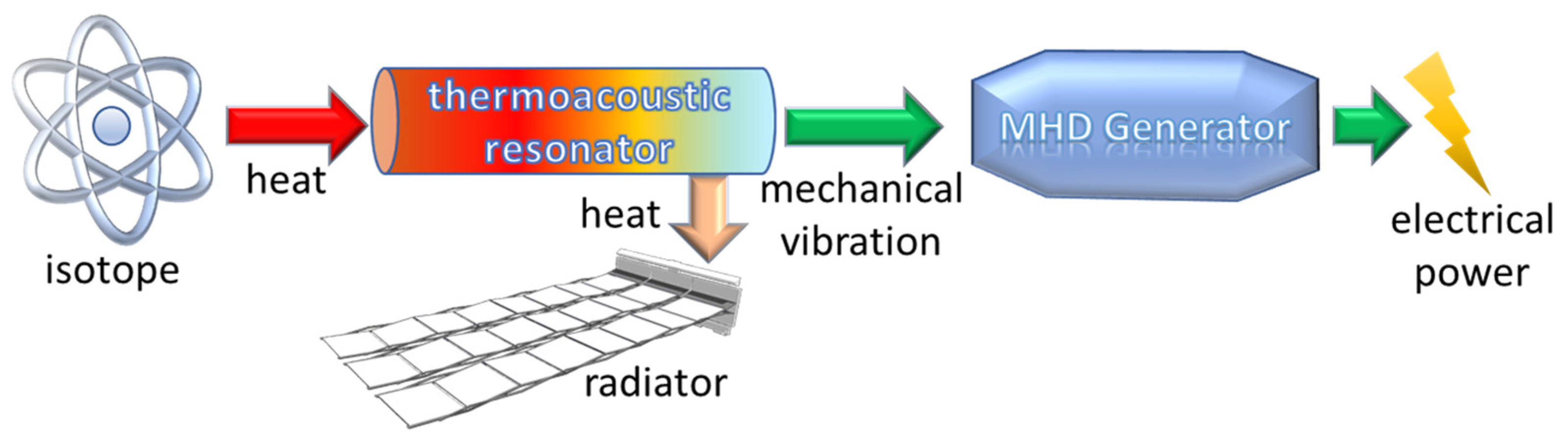
1. Introduction

The necessity to benefit from electricity in space is evident for various types of applications. The power supply of rovers for Mars missions is one example where the alternation of nights and days and dust storms create difficulties in the use of solar radiation. The possibility to have a long lifetime of thermal power, which can be used as the primary energy in an electrical generator, was the main objective of the EU-FP7 project SpaceTRIPS (2013–15 ID: 312639). The radioisotope americium able to supply thermal energy over several centuries was investigated. The global system (Figure 1), which was studied, was composed by:

• Americium heat source.
• Thermoacoustic engine, transforming thermal into mechanical energy.
• MHD generator, transforming mechanical energy into electrical one.
• Cold source, based on the thermal radiation in space.

The study involved a group composed of specialists of all parts. The americium heat source was under the responsibility of AREVA TA (Fr). The thermoacoustic engine (TAc) was dimensioned by the French company HEKYOM. The design study was done by the technical services (the SERAS) of the CNRS Grenoble (Fr). The MHD generator configuration was one of the main charges of HEKYOM and the Institute of Physics of the University of Latvia (IPUL) and was designed also by the SERAS. The radiative cold heat exchanger has been under the responsibility of Thales Alenia Space Torino (It), the Helmholtz-Zentrum Dresden-Rossendorf laboratory (HZDR) were involved with an important stability problem, explained later. All construction and tests were under the responsibility of IPUL. The present paper is specifically devoted to the calculation, description of the MHD electrical generator. The following Figure 1 summarizes the chain of elements that composed the project.

The novelty of the proposed system lies in the two stages of energy conversion, the former consisting of a thermoacoustic process that transforms the heat into mechanical energy, the latter one of a conversion of the mechanical energy into electricity. Both the stages are performed by devices with no moving parts. In the following section, the two processes are described in detail.

2. Materials and Methods

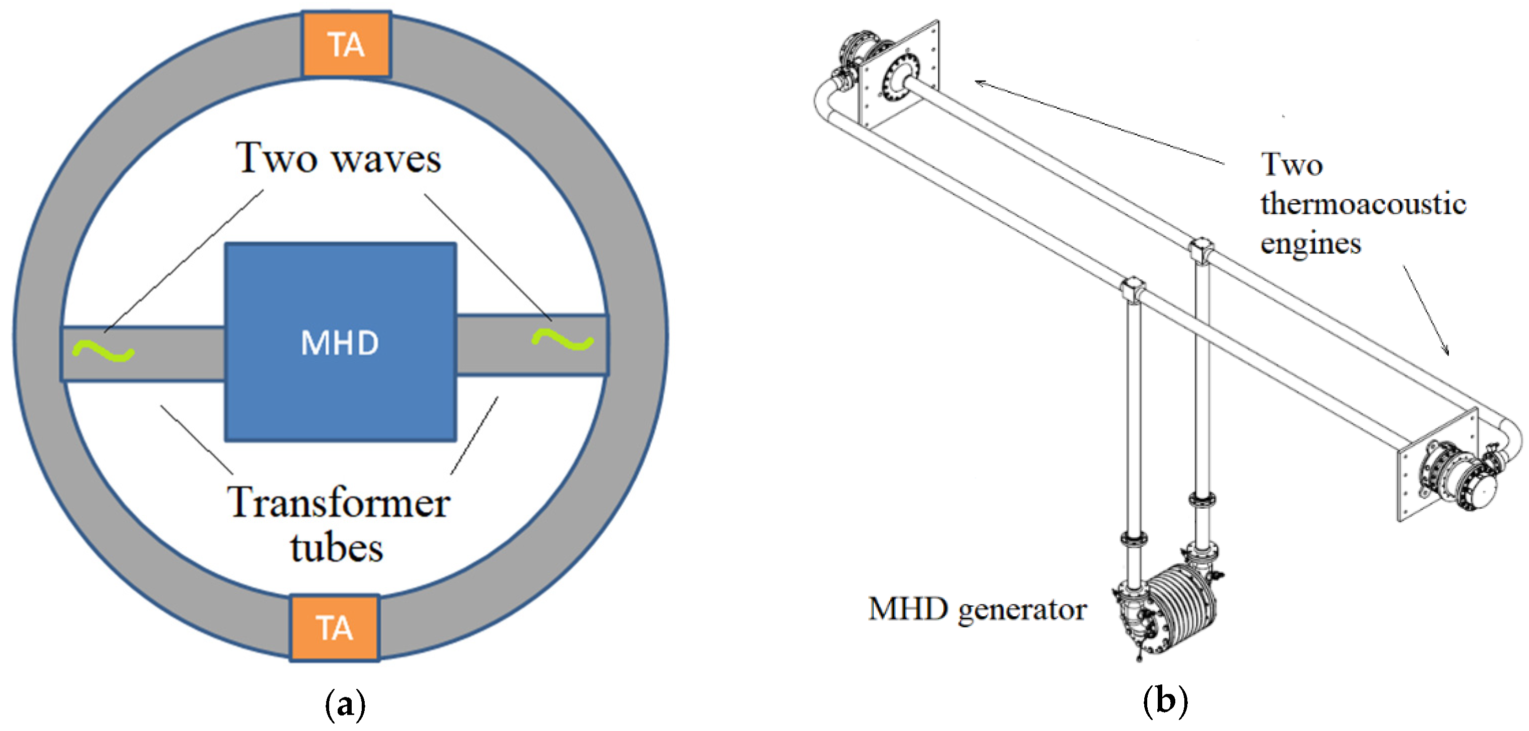
2.1. Description of the Thermoacoustic Engine

A thermoacoustic engine is a thermodynamic machine. When a high-temperature gradient is imposed on both extremities of an element with low thermal conductivity, called regenerator or stack, an acoustic wave is generated, which propagates in a pipe containing a gas at high pressure [1,2]. Two layouts are possible: linear (standing wave) or toroidal (traveling wave). The frequency of the oscillations depends consequently on both the sound velocity in the media and the length of the tube [3]. The engine is composed essentially of 4 elements:

(1)

A hot heat exchanger—connected with the hot source. In the SpaceTRIPS project, the heat source is expected to be americium elements. A prototype of the system has been built and tested in laboratory, where the isotope source has been simulated by a set of electrical resistances.

(2)

A cold heat exchanger—connected with the cold source, i.e., the radiative cooler. In the prototype it was simulated by water circulation.

(3)

A regenerator connected between the hot and the cold source, and then it is subject to a gradient of temperature.

(4)

A tube containing a gas. Helium is a good candidate due to its thermal properties [4], but Argon was adopted in the present project due its greater density, and further important properties that will be described in the following.

To be efficient, the gas must be involved at high pressure, partially because the heat transfer is better when the gas density is high. In addition, the mechanical energy generated by the resonator is proportional to the oscillating pressure, which is admitted by varying in the range by 5 to 10% of the average value. Consequently, a mean pressure of 40 bar could give oscillating pressure around 2 to 4 bar, which corresponds to a suitable value of the generated power.

As for any thermodynamic system, the maximum efficiency is expressed by the Carnot’s formula in function of the range of temperatures.

For reasons that will be given in the following paragraph, arising from the use of Sodium in the MHD generator, the cold source will be around 100 °C. Therefore, expecting a global efficiency around 50% of the Carnot efficiency, the details of the performance are proposed in

Table 1. Main design parameters of the Space TAc-MHD generator.

Gas in the TAc Engine	Liquidin MHD Generator	Temp. Hot Source	Temp.ColdSource	Pressure Oscillations	Mean Pressure	Carnot Efficiency	ExpectedGlobal Efficiency	Level of Electrical Power	Efficiency of MHD Generator	MechanicalEnergy (TAc Engine)	Efficiency of the TAc Engine
Argon	Sodium	800 °C	150 °C	+/−3 bar	40 bar	0.66	0.25	200 W	0.7	300 W	0.4

below.

The chosen configuration of the TAc engine is given in Figure 2a,b. For thermodynamics consideration [5,6], the thermoacoustic wave is traveling in a closed tube. Two thermoacoustic wave engines were involved, working in push–pull configuration. The MHD generator was located along a “diameter” of the closed loop and consequently both the ends of the generator were subject to an oscillating pressure, which are phase shifted of 180° one each other. The oscillating pressure applied to the ends of the MHD generator performs as the motor of the system.

The corresponding mechanical energy corresponds to the product ΔP × Q_Ar, where ΔP is the pressure difference between the two ends of the electrical generator and Q_Ar is the oscillating flowrate of argon.

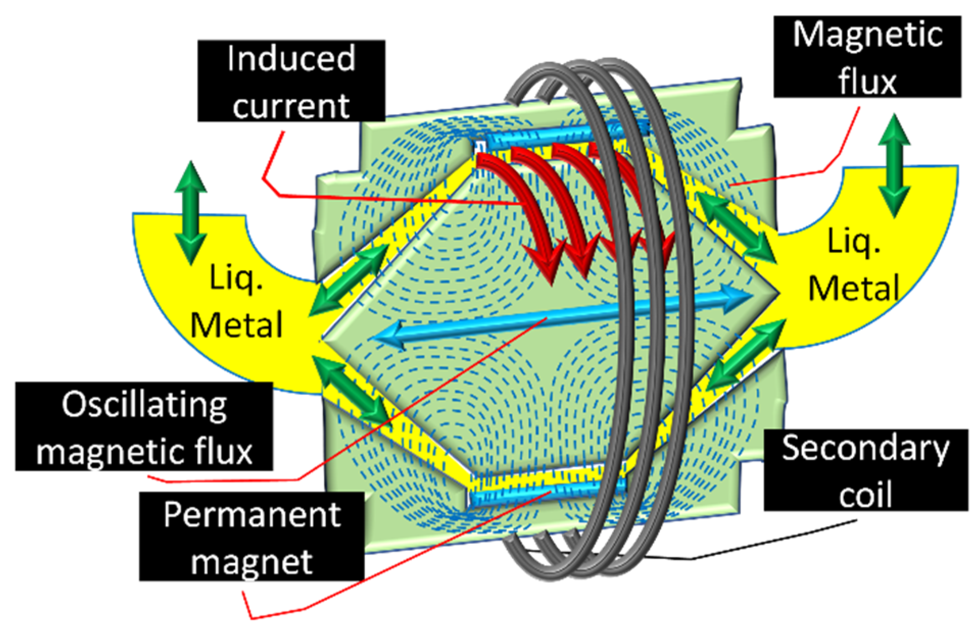
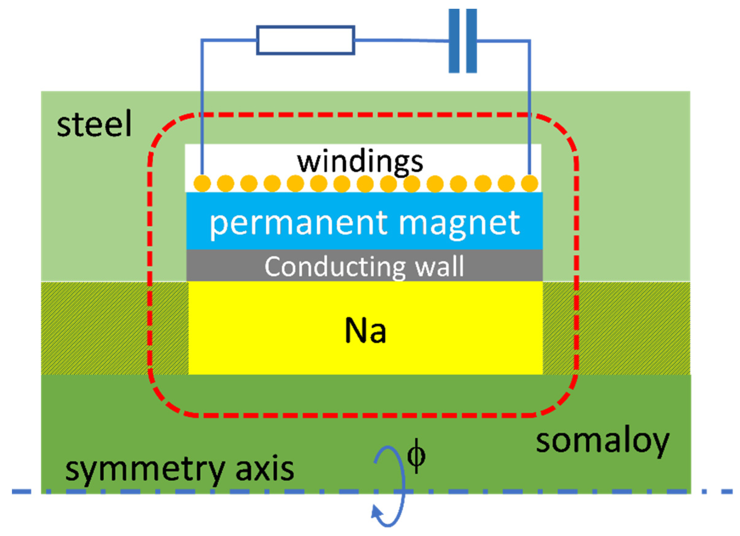
2.2. Description of the MHD Generator

The mechanical energy is converted into electricity by a liquid-metal, inductive MHD generator. A schematic representation of the principle of operation is given in Figure 3. The pulsating pressure and velocity produced by the TAc engine are applied to both the ends of a duct filled with liquid sodium [7,8]. This duct is tapered in the middle, to raise the velocity of the sodium in the operating zone. The oscillating sodium is submitted to a radial DC magnetic field generated by a toroidal permanent SmCo magnet. The magnetic streamlines close through the high magnetic permeability material (somaloy [9,10]) and then through a package of typical sheets of high magnetic permeability used for the transformers. The motion of the liquid sodium in the DC magnetic field induces in the sodium itself an AC toroidal current, which generates an AC magnetic field. An external coil, coaxial with the permanent magnet, performs as the secondary of a transformer, while the current circulating in the liquid sodium works as the primary coil. The transformation chain terminates with an electrical load connected to the external coil. A capacitor must be connected to the load for the power factor correction.

This kind of generator has several reasons of interest. Firstly, there is no contact between the sodium and the exterior of the generator, which is an important aspect, due to the high reactivity of the sodium with water. Secondly, the power is transmitted by induction, therefore it does not need electrodes to capture electrical current, which is one of the main issues of the conventional MHD generators [11,12,13]. Finally, as for the TAc engine, there are no solid moving parts, therefore the entire process chain is quasi static, which represents a very important advantage for space applications [14].

2.3. Analytical Model of the MHD Generator

In this section, a simplified analysis of the MHD generator is performed by means of a one-dimensional model. In

Table 2. Variables of the model.

Symbol	Description of Parameter	Value
B	Magnetic field induction in sodium gap	[0.33 T]
B0	Magnetic field induction in somaloy	[T]
μ0	Somaloy relative magnetic permeability	200
l0	Length of magnetic streamlines through somaloy	[0.06 m]
S0	Somaloy cross section	[0.009852 m2]
Bf	Induced field in steel	[T]
μf	Steel relative magnetic permeability	3280
lf	Length of magnetic streamlines through steel	[0.06 m]
Sf	Steel cross section	[$5.7555\times {10}^{-3}$ m2]
Be	Induced field in converging duct	[T]
le	Length of magnetic streamlines in sodium	[$2\times {10}^{-3}$ m]
Se	Converging duct cross section	[$5.538\times {10}^{-3}$ m2]
Ss	Toroidal gap (and free surface) cross section	[$1.432\times {10}^{-3}$ m2]
I1	Electrical current induced in the sodium	[A]
I2	Electrical load current	[A]
Iw	Electrical current in the titanium wall	[A]
n	Number of coil turns	[400]
Φ0	Magnetic flux	[Wb]
r1	Sodium resistance	[0.2475 mΩ]
r2	Load resistance (MHD generator coil-9 Ω)	[Ω]
rw	Titanium sheet resistance	[2.95 mΩ]
D	Toroidal channel diameter	[0.114 m]
V	Sodium velocity	[m/s]
q	Charge on load capacitor	[C]
C	Load capacity	[F]
ω	AC oscillation angular frequency	[314 rad/s]
m	Sodium mass	[0.464 kg]
ΔP	Applied pressure	[Pa]
ν	Sodium kinematic viscosity	[$0.77\times {10}^{-6}$ m2/s]
ρ	Sodium density	[928 kg/m3]

, the list of the variables and the corresponding values are reported.

Equation (1) is related to the Ampere theorem: the induced magnetic field is produced by the induced electric current in the Sodium. Let us consider a magnetic streamline (red dashed line in Figure 4). Three electrical currents cross the area delimited by the magnetic streamline: the electric current in the sodium I₁; the induced electric current in the thin conducting wall I_w, and the induced electric current in the coil I₂; “n” being the number of turns of the coil. More detailed formula notations are described below.

The Ampere’s theorem for magnetic flux line writes:

$$\frac{B_0}{{\mu }_0}{l}_0+\frac{B_f}{{\mu }_f}{l}_f+2\frac{B_e}{{\mu }_0}{l}_e=I_1+I_{2}n+I_w,$$

(1)

Using the principle of magnetic flux conservation:

$$B_f{S}_f=B_e{S}_e=B_0{S}_0,$$

(2)

S₀ being somaloy cross section, S_f the steel cross section, S_e the Na subchannel cross section, and μ₀ the somaloy magnetic permeability. From (1) and (2):

$$B_0\left(l_0+\frac{{\mu }_0{S}_0}{{\mu }_f{S}_f}{l}_f+2\frac{S_0}{S_e}{l}_e\right)={\mu }_0\left(I_1+I_{2}n+I_w\right)$$

(3)

Let us call “equivalent length” the following term:

$$L_0^{\prime }=l_0+\frac{{\mu }_0{S}_0}{{\mu }_f{S}_f}{l}_f+2\frac{S_0}{S_e}{l}_e.$$

(4)

Then, the magnetic flux can be expressed as:

$$\Phi =\frac{S_0}{L_0^{\prime }}{\mu }_0\left(I_1+I_{2}n+I_w\right).$$

(5)

By considering separately the electrical circuits corresponding to the electric currents I₁, I₂, I_w, the following 3 equations are obtained:

• The current I₁ corresponds to a toroidal channel filled with sodium with mean diameter D and internal resistance r₁. The applied induction field B interacts with the sodium that oscillates with velocity V:

  $$I_1{r}_1+\pi DVB=-\frac{d\Phi }{dt}.$$

  (6)
  After deriving:

  $$-\frac{d^2\Phi }{d{t}^2}=r_1\frac{d{I}_1}{dt}+\pi DB\frac{dV}{dt}.$$

  (7)
• The circuit formed by the coil, the load, and the power factor correction capacity have a total resistance R and a capacitance C such that C∙U = q:

  $$I_2{r}_2+\frac{q}{C}=-n\frac{d\Phi }{dt}.$$

  (8)
  Again, after deriving:

  $$-\frac{d^2\Phi }{d{t}^2}=\frac{r_2}{n}\times \frac{d{I}_2}{dt}+\frac{I_2}{nC}.$$

  (9)
• Finally, the circuit constituted by the thin conducting wall of internal resistance r_w:

  $$r_w{I}_w=-\frac{d\Phi }{dt}.$$

  (10)
  Again, after deriving:

  $$-\frac{d^2\Phi }{d{t}^2}=\frac{r_{w}d{I}_w}{dt}.$$

  (11)

2.4. Solution of the Model

The Equations (3)–(11) can be combined to obtain the following 3 equations:

$$\frac{d^2\Phi }{d{t}^2}=\frac{S_0}{L_0^{\prime }}{\mu }_0\left(\frac{d^2{I}_1}{d{t}^2}+n\frac{d^2{I}_2}{d{t}^2}+\frac{d^2{I}_w}{d{t}^2}\right)=-\left(\frac{r_2}{n}\times \frac{d{I}_2}{dt}+\frac{1}{nC}{I}_2\right),$$

(12)

$$\frac{r_{1}d{I}_1}{dt}+\frac{\pi DBdV}{dt}=\frac{r_2}{n}\times \frac{d{I}_2}{dt}+\frac{1}{nC}{I}_2,$$

(13)

$$\frac{r_{w}d{I}_w}{dt}=\frac{r_2}{n}\times \frac{d{I}_2}{dt}+\frac{1}{nC}{I}_2.$$

(14)

The Equations (12)–(14) describe the main physical properties of the process. By calling ϕ the phase shift between sodium velocity $V=V_0{e}^{i\omega t}$ and the current in the load $I_2=I_0{e}^{i\left(\omega t+\varphi \right)},$ and introducing:

$$\alpha =r_2\left(\frac{1}{n^2{r}_1}+\frac{1}{n^2{r}_w}\right)+1,$$

(15)

$$\beta =\frac{1}{C}\left(\frac{1}{n^2{r}_1}+\frac{1}{n^2{r}_w}\right),$$

(16)

the following solution is obtained:

$$I_0=\frac{n{S}_0{\mu }_0{\omega }^2}{L_0^{\prime }\mathit{cos}\varphi \left[n^2\frac{S_0}{L_0^{\prime }}{\mu }_0\left(\alpha {\omega }^2+\beta \omega tg\varphi \right)-\frac{1}{C}+r_2\omega tg\varphi \right]}\times \frac{\pi DB{V}_0}{r_1},$$

(17)

$$tg\varphi =\frac{r_2{L}_0^{\prime }\omega +n^2{S}_0{\mu }_0\omega \beta }{n^2{S}_0{\mu }_0{\omega }^2\alpha -\frac{L_0^{\prime }}{C}}.$$

(18)

The velocity depends on the pressure oscillations applied at the ends of the electrical generator and on the interaction with the applied magnetic field. The difference of pressure between the ends of the generator writes:

$$\Delta P e^{i \left(\omega t+\psi \right)}$$

(19)

The fundamental equation of the mechanics gives:

$$\Delta P{S}_s-I_1\pi DB-KV=m\frac{dV}{dt},$$

(20)

where K is the friction coefficient. By deriving with respect to time:

$$\frac{d\Delta P}{dt}{S}_s-\pi DB\frac{d{I}_1}{dt}-K\frac{dV}{dt}=m\frac{d^{2}V}{d{t}^2}.$$

(21)

Then, by using Equation (13):

$$\frac{d{I}_1}{dt}=\frac{r_2}{n{r}_1}\times \frac{d{I}_2}{dt}+\frac{I_2}{n{r}_{1}C}-\frac{\pi DB}{r_1}\frac{dV}{dt},$$

(22)

$$\frac{d{I}_1}{dt}=\frac{r_2}{n{r}_1}\times I_{0}i\omega e^{i\left(\omega t+\varphi \right)}+\frac{1}{n{r}_{1}C}{I}_0{e}^{i\left(\omega t+\varphi \right)}-\frac{\pi DB{V}_0}{r_1}i\omega e^{i\left(\omega t\right)},$$

(23)

$$\frac{d{I}_1}{dt}=I_{0}i\omega e^{i\left(\omega t+\varphi \right)}\left(i\omega \frac{r_2}{n{r}_1}+\frac{1}{n{r}_{1}C}\right)-\frac{\pi DB{V}_0}{r_1}i\omega e^{i\left(\omega t\right)}.$$

(24)

By resorting to the phasorial notation, the Equation (21) gives:

$$\begin{gathered} \Delta P{S}_{s}i\omega e^{i\left(\omega t+\psi \right)}-\pi DB\left(I_0{e}^{i\left(\omega t+\varphi \right)}\left(i\omega \frac{r_2}{n{r}_1}+\frac{1}{n{r}_{1}C}\right)-\frac{\pi DB}{r_1}{V}_{0}i\omega e^{i\left(\omega t\right)}\right) \\ -Ki\omega V_0{e}^{i\left(\omega t\right)}=-m{\omega }^2{V}_0{e}^{i\left(\omega t\right)} \end{gathered}$$

(25)

By simplifying the common term $e^{i\left(\omega t\right)}$ and inserting sodium current I₀ expression (17):

$$\begin{gathered} \Delta P{S}_{s}i\omega e^{i\psi }-\pi DB\times \frac{n{S}_0{\mu }_0{\omega }^2}{L_0^{\prime }\mathit{cos}\varphi \left[n^2\frac{S_0}{L_0^{\prime }}{\mu }_0\left(\alpha {\omega }^2+\beta \omega tg\varphi \right)-\frac{1}{C}+r_2\omega tg\varphi \right]} \\ \times \frac{\pi DB{V}_0}{r_1}{e}^{i\varphi }\left(i\omega \frac{r_2}{n{r}_1}+\frac{1}{n{r}_{1}C}\right)+\frac{{\left(\pi DB\right)}^2}{r_1}{V}_{0}i\omega -Ki\omega V_0=-m{\omega }^2{V}_0 \end{gathered}$$

(26)

It is possible to express V₀ and Ψ versus ΔP from the real and imaginary part of Equation (26):

$$\begin{gathered} tg\psi =-\left[\left(\begin{array}{l}\frac{S_0{\mu }_0{\omega }^2}{L_0^{\prime }\mathit{cos}\varphi \left[n^2\frac{S_0}{L_0^{\prime }}{\mu }_0\left(\alpha {\omega }^2+\beta \omega tg\varphi \right)-\frac{1}{C}+r_2\omega tg\varphi \right]}\times \frac{{\left(\pi DB\right)}^2}{r_1}\cdot \\ \times \left(-\omega \mathit{sin}\varphi \frac{r_2}{r_1}+\frac{\mathit{cos}\varphi }{r_{1}C}\right)\end{array}\right)-m{\omega }^2\right]\cdot \\ \frac{1}{\left[\left(\begin{array}{l}\frac{S_0{\mu }_0{\omega }^2}{L_0^{\prime }\mathit{cos}\varphi \left[n^2\frac{S_0}{L_0^{\prime }}{\mu }_0\left(\alpha {\omega }^2+\beta \omega tg\varphi \right)-\frac{1}{C}+r_2\omega tg\varphi \right]}\times \frac{{\left(\pi DB\right)}^2}{r_1}\cdot \\ \times \left(\omega \mathit{cos}\varphi \frac{r_2}{r_1}+\frac{\mathit{sin}\varphi }{r_{1}C}\right)\end{array}\right)-\omega \times \left(\frac{{\left(\pi DB\right)}^2}{r_1}-K\right)\right]} \end{gathered}$$

(27)

$$V_0=\frac{-\Delta P{S}_s\omega \frac{tg\psi }{\sqrt{\left(1+tg{\psi }^2\right)}}}{\left[\left(\begin{array}{l}\frac{S_0{\mu }_0{\omega }^2}{L_0^{\prime }\mathit{cos}\varphi \left[n^2\frac{S_0}{L_0^{\prime }}{\mu }_0\left(\alpha {\omega }^2+\beta \omega tg\varphi \right)-\frac{1}{C}+r_2\omega tg\varphi \right]}\times \frac{{\left(\pi DB\right)}^2}{r_1}\cdot \\ \times \left(-\omega \mathit{sin}\varphi \frac{r_2}{r_1}+\frac{\mathit{cos}\varphi }{r_{1}C}\right)\end{array}\right)-m{\omega }^2\right]}.$$

(28)

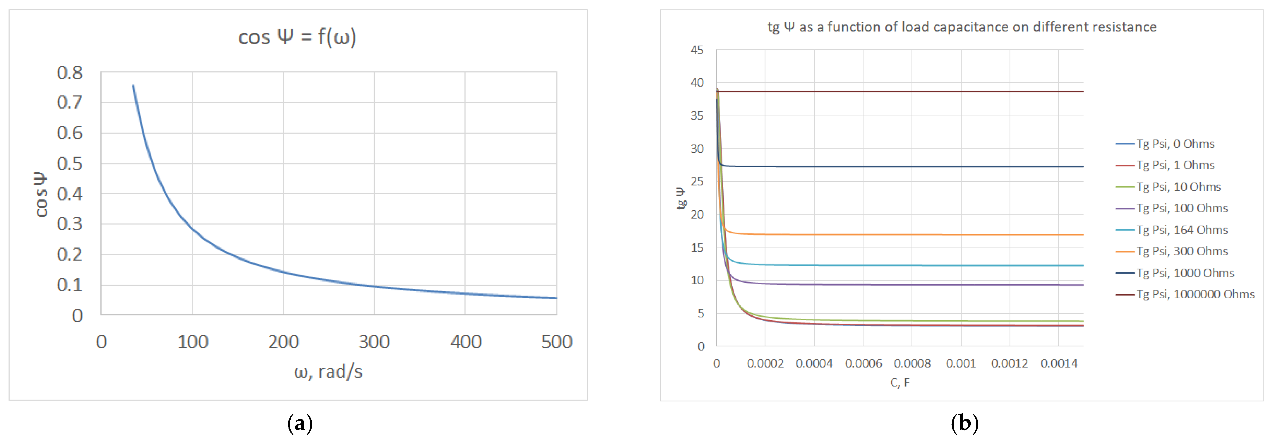
2.5. Remark about the Angle ψ

The angle ψ is an important parameter, which is related to the electrical power that can be extracted from the system. Indeed, it characterizes the mechanical energy introduced into the MHD generator. This energy is proportional to the scalar product $\overrightarrow{\Delta P}·\overrightarrow{V}$. To optimize the power conversion, cos ψ must be as large as possible. In Figure 5a,b, it can be observed that, when the mass of sodium is relevant, as in the present case, only low frequencies are suitable. Therefore, a significant effort should be made to optimize the system. It is also worth noting that for the operative conditions in the present experiment, acceptable values of cos ψ can only be obtained for low values of the load resistance. It is also important to note that the parameter ψ does not affect the efficiency of the generator, but it only limits the inlet mechanical power, and consequently the producible electric power.

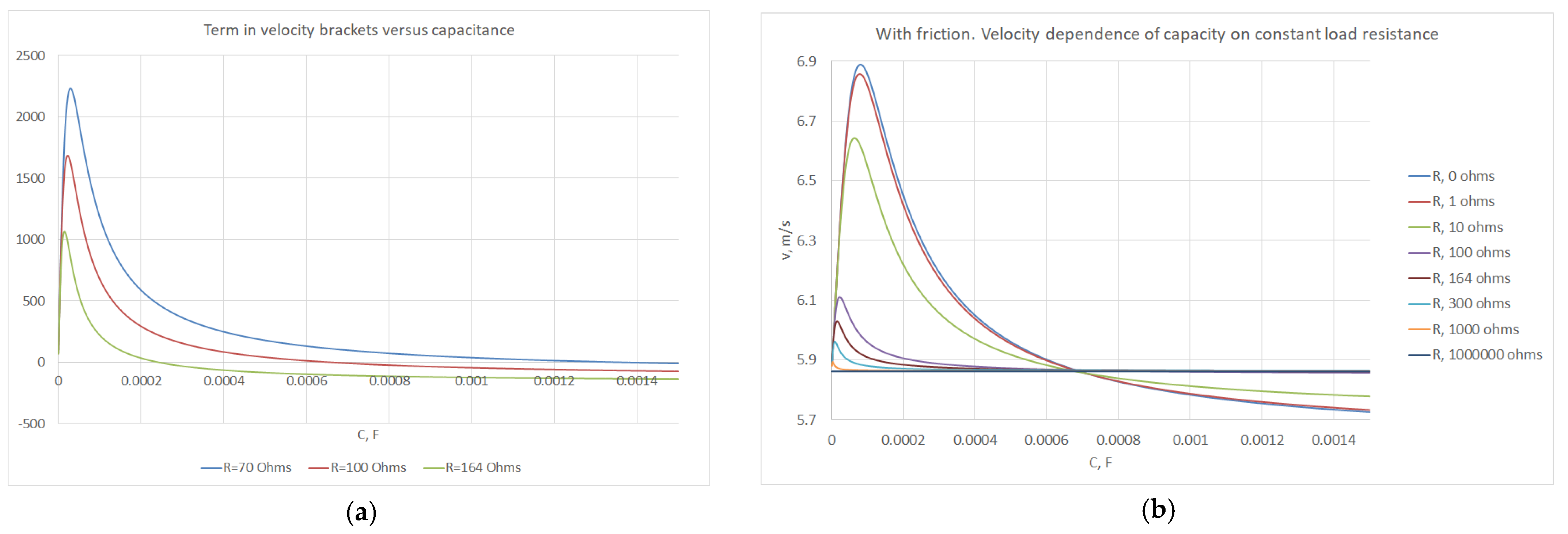
2.6. Velocity

For C = 0, there is no current in the circuit, because $Q=C U->dQ / dt=I2=0$ and therefore the system, and in particular the velocity, does not depend on the load. Consequently, for low values of C, dV/dC for C = 0 is practically constant, because the induced current in the sodium is only slightly influenced by the capacitance.

This is confirmed by the fact that, as can be seen, tgψ is always very high and consequently $\frac{tg\psi }{\sqrt{1+tg{\psi }^2}}=sin \psi ~ 1$. Therefore, according to the expression (28), when C tends to zero, the velocity depends only on the applied pressure and inertia of the sodium in agreement with the affirmation given above. It is worth to say that when there is no current in the load, the totality of mechanical energy must be dissipated in the sodium by the Joule’s effect. By the consequence, the electric current must be high enough, then the electromagnetic force opposite to the pressure forces is also high. Therefore, the velocity becomes relatively small. This result can be observed on Figure 6b.

Figure 6b reveals that for two values of C, the velocity seems to be independent of the load resistance (this comes from the fact that the term in the parenthesis at the denominator of the velocity Expression (28) becomes null for two values of the capacity). The first value is C = 0, while the second one depends on the load resistance. From a physical point of view, this capacitance value equilibrates exactly the apparent inductance, which is the combination of all the inductances present in the system. In these conditions, the velocity (critical velocity) is only controlled by inertia and becomes independent of the load resistance. That fits well with the results that can be seen in Figure 6b. It is also worth noting that for small r₂, the apparent inductance does not depend too much on the load. However, for higher values of the load, the second values of C increases when r₂ increases (Figure 6a). Nevertheless, this does not considerably affect the critical value that is maintained very close to the one obtained for small loads. More generally, from the results comes that, regardless of capacity and load, the velocity ranges between 5.8 to 6.9 m/s. This means that the inertia terms are still dominant and probably should be reduced by reducing the mass of sodium for better efficiency. Lastly, we remark about the velocity: when C tends to infinity, the capacity does not play any role and, all things being equal, V₀ is constant with a value that depends exclusively on the load resistance.

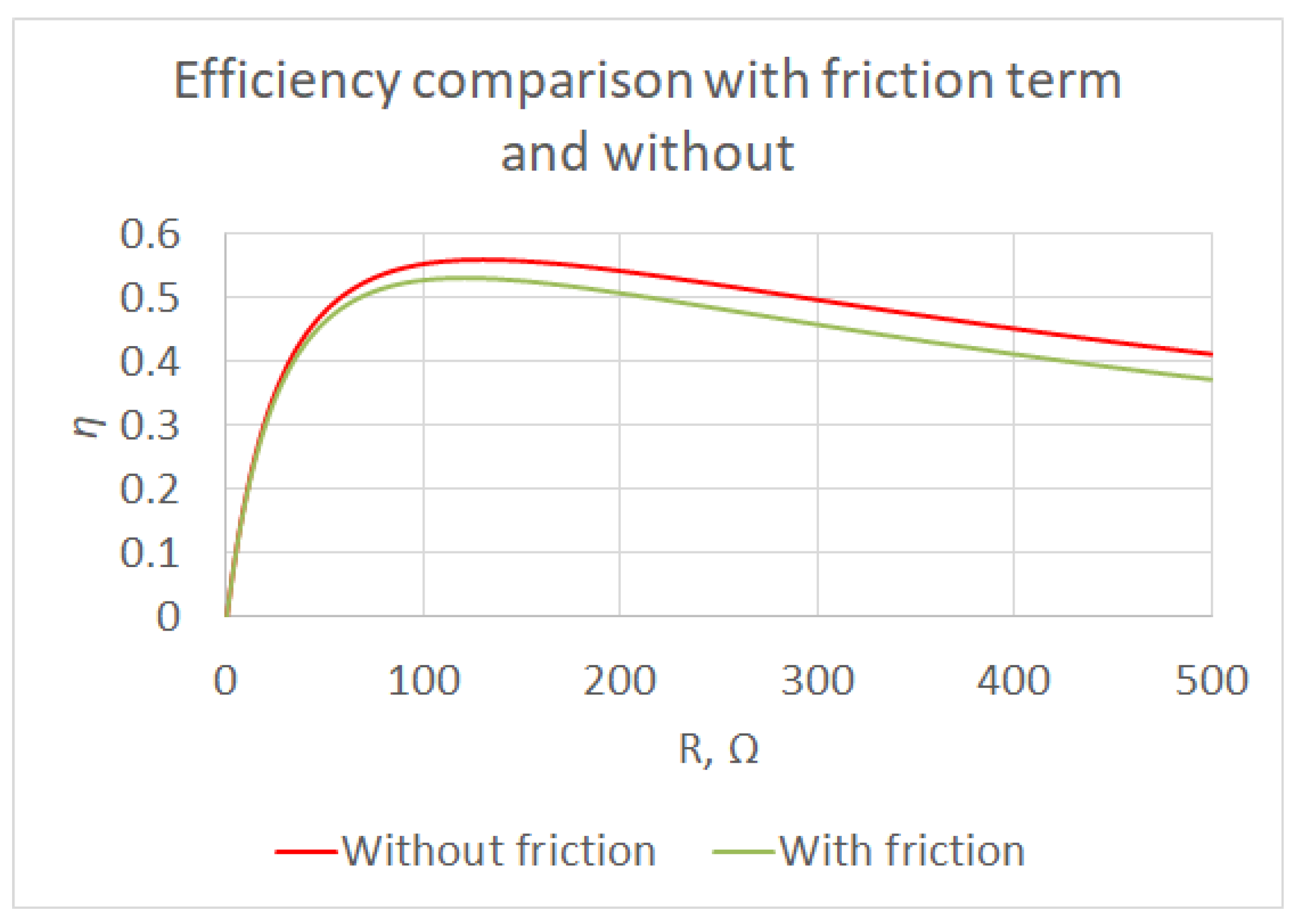
2.7. Friction

The coefficient K, which represents the friction at the wall, depends on the characteristics of the flow and on the size $\delta$ of the hydrodynamic boundary layer, which is controlled by the angular frequency ω in competition with the kinematic viscosity ν:

$$\delta ~\sqrt{\frac{\nu }{\omega }}.$$

(29)

The friction force is not always opposite to the flow. To estimate that, it is possible to characterize the typical time of an oscillation:

$${\tau }_{osc}~\frac{2\pi }{\omega }$$

(30)

Additionally, to compare with the typical time to transfer the influence of the viscosity at the wall to the center of the flow (typical size d).

$${\tau }_{\nu }~\frac{d}{\sqrt{\omega \nu }}$$

(31)

If ${\tau }_{\nu }\gg {\tau }_{osc} \to \frac{d}{2 \pi } \sqrt{\frac{\omega }{ \nu }}\gg 1$. In this case, the direction of the flow changes before the effect of viscosity is manifest. Then, for a while the friction at the wall is a positive term, while it is opposite to the flow in the rest of the period. This is the reason why the influence of the viscosity was attenuated by a factor 2 in the calculation. However, in any case this influence is very low, as it can be seen on Figure 13b. The term becomes relevant for the efficiency only for very low values of the applied magnetic field.

The friction force τ by unit of surface has an order of magnitude:

$$\tau ~\rho \nu \frac{V_0}{\delta }\to \tau ~\rho \nu \frac{V_0}{\sqrt{\frac{\nu }{\omega }}}=\rho \sqrt{\nu \omega }{V}_0$$

(32)

From $\tau$ it is easy to deduce:

$$F_{\nu }=\tau S=K{V}_0,$$

(33)

where S the interface between sodium and walls. Then, friction power and friction coefficient are:

$$F_{\nu }=\rho \sqrt{\nu \omega }{V}_{0}S\to K=\frac{1}{2}\rho \sqrt{\nu \omega }S$$

(34)

If the frequency of the oscillations is high, the influence of viscosity at the wall does not have time to be felt at the level of the core of the flow before the change in direction of the latter. Therefore, during this short time, the forces of viscosity are driving, and not resisting, explaining the choice of the coefficient ½ in front of the friction coefficient K [15,16]. This question needs to be studied in more detail in the future. In the newest literature there is an attractive design example proposed, where mechanical and hydrodynamic friction is fully eliminated by replacing the liquid metal with oscillating electrically conductive gas, driven by thermoacoustic engine [17,18,19]. Other interesting examples on MHD power generation using ocean wave energy are described in [20,21,22].

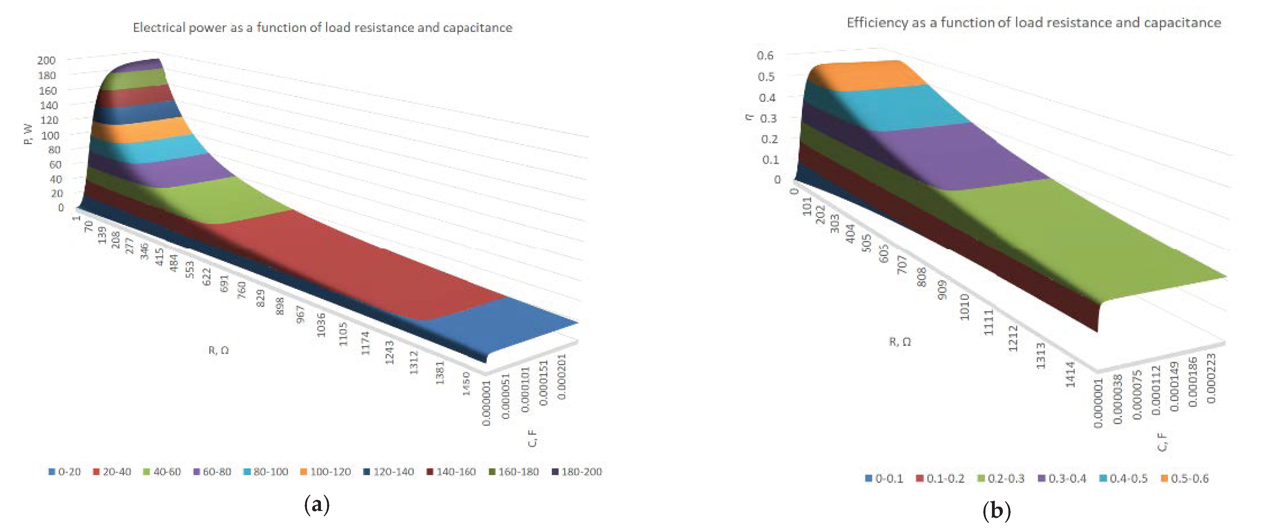
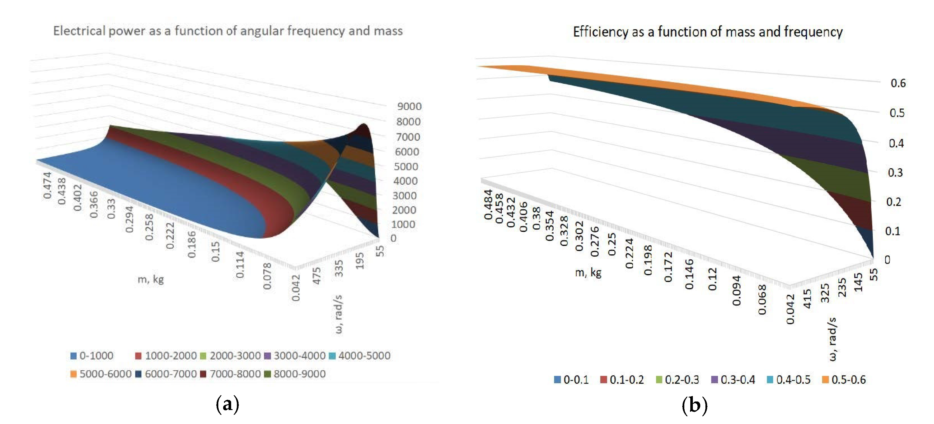
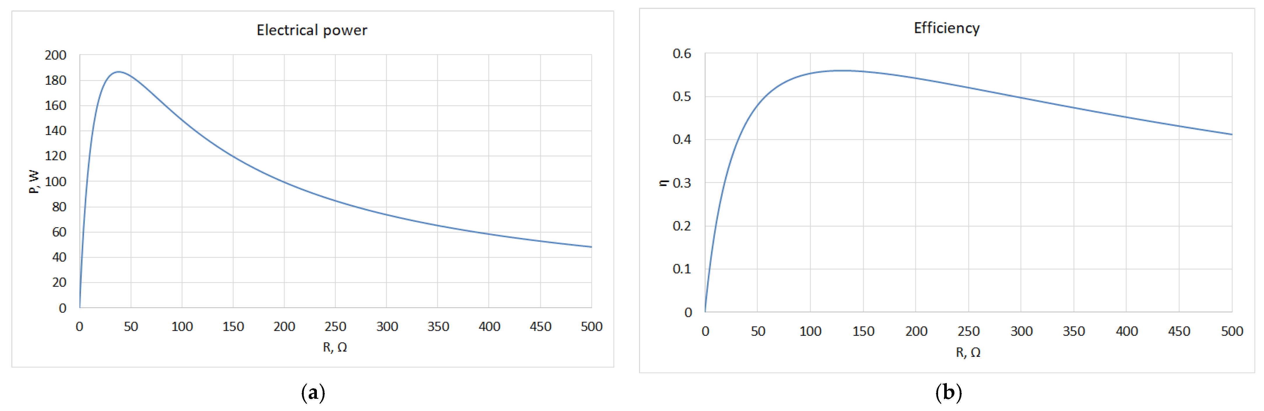
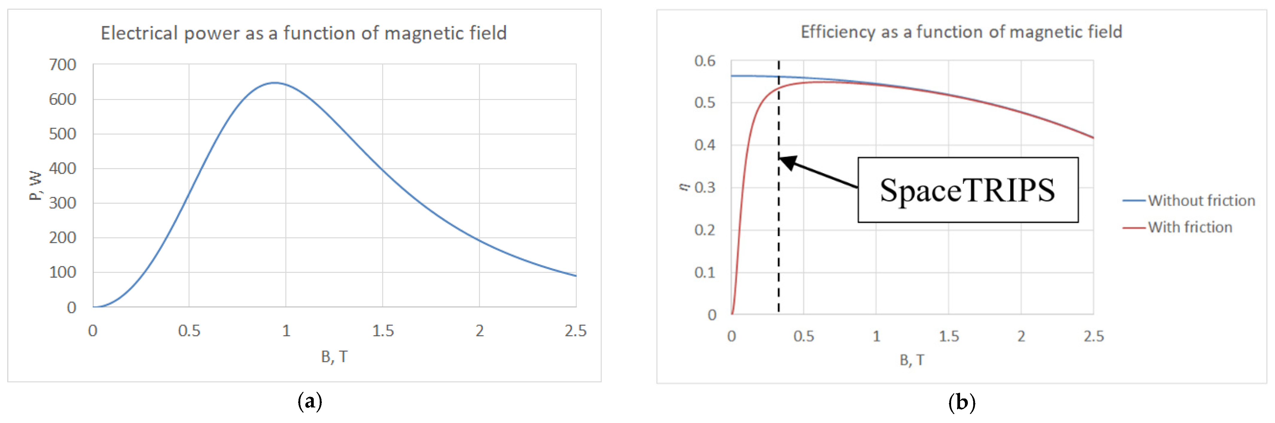
2.8. Efficiency Analysis

The most important parameter is the global efficiency of the process. This parameter is defined as the ratio of the electrical power available at the load by the mechanical energy from the thermoacoustic waves. Writing Equation (20) in the form:

$$\Delta P{S}_s{e}^{i\psi }-\pi DB{I}_{1o}{e}^{i\theta }-K{V}_0=mi\omega V_0,$$

(35)

exhibits the parameter θ, which is the phase shift between the electrical current in the sodium and velocity. It is possible to estimate the value of cos θ. Considering the Ohm’s law:

$$j=\sigma \left(\overrightarrow{E}+\overrightarrow{V}\wedge \overrightarrow{B}\right),$$

(36)

and assuming that:

$$j=\frac{I}{S},$$

(37)

where S-cross section of the channel and$I=I_{1o}{e}^{i\theta },$ and using Maxwell equation:

$$rot \overrightarrow{E }=-\frac{\partial b}{\partial t},$$

(38)

after very simple manipulations allows us to write:

$$\frac{I_{1o}}{S}{e}^{i\theta }~ \sigma \left(i \omega b l+V_o{B}_o\right),$$

(39)

and considering that, for small magnetic Reynolds number, the induced field b is lower than the applied one:

$$Rm=\frac{b}{B_o} ~ \mu \sigma B_o l\ll 1,$$

(40)

were “l” being a typical scale of the system. One obtains finally:

$$e^{i\theta }~ \left(\frac{i \omega b l}{V_o{B}_o}+1\right)\frac{\sigma V_o{B}_o}{I_{1o}} S \to \sigma \left(i \omega l^2 \mu \sigma +1\right)\frac{\sigma V_o{B}_o}{I_{1o}} S.$$

(41)

If:

$$\omega \mu \sigma l^2=R{m}^{*}\ll 1,$$

(42)

and consequently:

$$\frac{I_{1o}}{S} ~ \sigma V_o{B}_o,$$

(43)

the induced current in the sodium due to the pulsation of the induced magnetic field is lower than the imposed one due to the interaction between the sodium velocity and the imposed magnetic field, which agrees with the Lenz’s law considering that the imposed current is the source term. In these conditions, θ ~ 0.

Returning to the efficiency estimation, the friction term can be assimilated to an electromagnetic force with an equivalent current on the form:

$$\frac{K{V}_0}{\pi D{B}_0}.$$

(44)

According to that, the dynamics equation of the motion can be written:

$$\Delta P{S}_s{e}^{i\psi }-\pi D{B}_0\left(I_{1o}{e}^{i\theta }-\frac{K{V}_0}{\pi D{B}_0}\right)=mi\omega V_0.$$

(45)

In Equation (45), there are two terms in brackets: the first one proportional to $I_{1o}$ represents the true electromagnetic force, while the second one, $K{V}_0/\pi D{B}_0$, is called equivalent electric current, and it corresponds to the friction force.

Converting to trigonometric form:

$$\Delta P{S}_s\left(\mathit{cos}\psi +i\mathit{sin}\psi \right)-\pi D{B}_0{I}_{1o}\left(\mathit{cos}\theta +i\mathit{sin}\theta \right)-K{V}_0=mi\omega V_0,$$

(46)

and after separating real and imaginary parts gives the real part:

$$\Delta P{S}_s\mathit{cos}\psi =I_{1o}\mathit{cos}\theta \pi D{B}_0+K{V}_0,$$

(47)

but if $\theta \to 0$, then:

$$\Delta P{S}_s\mathit{cos}\psi -K{V}_0\approx I_{1o}\pi D{B}_0.$$

(48)

and imaginary part:

$$\Delta P{S}_s\mathit{sin}\psi -m\omega V_0=I_{1o}\mathit{sin}\theta \pi D{B}_0$$

(49)

but if θ→0, then:

$$\Delta P{S}_s\mathit{sin}\psi -m\omega V_0\approx 0.$$

(50)

Taking the square of both equations, we can sum them up:

$${\left(\Delta P{S}_s\mathit{sin}\psi -m\omega V_0\right)}^2+{\left(\Delta P{S}_s\mathit{cos}\psi -K{V}_0\right)}^2={\left(I_{1o}\right)}^2{\left(\pi D{B}_0\right)}^2.$$

(51)

Allowing us to write the following expression for current in sodium:

$$I_{1o}=\sqrt{\frac{\begin{array}{c}{\left(\Delta P{S}_s\mathit{sin}\psi \right)}^2-2m\omega \Delta P{S}_s\mathit{sin}\psi V_0+{\left(m\omega V_0\right)}^2+{\left(\Delta P{S}_s\mathit{cos}\psi \right)}^2-\\ -2\Delta P{S}_s\mathit{cos}\psi K{V}_0+{\left(K{V}_0\right)}^2\end{array}}{{\left(\pi D{B}_0\right)}^2}}.$$

(52)

This expression can be simplified considering Equation (46):

$$\Delta P\times S_s\approx \frac{I_{1o}\pi D{B}_0+K{V}_0}{\mathit{cos}\psi } ,$$

(53)

from which can be extracted an equivalent form of $V_0$.

On the other hand, neglecting the friction leads to:

$$I_{1o}=\frac{\Delta P S_{s }cos\psi }{\pi D B_0},$$

(54)

and for very high values of C, the current in the sodium depends exclusively on the load resistance. The electromagnetic force equilibrates exactly the pressure force (also since cos ψ is almost constant with the value fixed by r₂). Consequently, the mechanical work introduced in the generator being equal to:

$$\frac{\Delta P S_{s }{V}_{0}cos\psi }{2},$$

(55)

takes also a constant value depending always about the load resistance (Figure 7b). Considering Equation (51), the mechanical power takes the form:

$$\frac{\Delta P S_{s }{V}_{0}cos\psi }{2}\approx \frac{(I_{1o }\pi D{B}_0+K{V}_0)V_0}{2}.$$

(56)

Therefore, the mechanical power appears like the sum of the work of electromagnetic forces and the friction forces.

The efficiency of the MHD generator is given by the electrical power in the load reported to the introduced mechanical power:

$$\eta =\frac{P_{elec}}{P_{mech}}=\frac{r_2{I}_0{}^2}{\Delta P{V}_0 S_s cos\psi }.$$

(57)

It is possible to express the efficiency in another form that corresponds also to the electrical power dissipated at the load reported to the sum of electrical energy at the load + at the wall + in the sodium itself + the dissipation due to the friction term. That gives:

$$\eta =\frac{r_2{I}_0{}^2}{r_2{I}_0{}^2+r_1{I}_1{}^2+r_w{I}_w{}^2+\frac{F_v V_0}{4} },$$

(58)

with $F_v$ the friction force. See Equation (31).

As it can be seen in Figure 8, the efficiency is not too much affected by the friction. Therefore, in the following the results will be proposed without friction.

Suppressing the capacity allows a great simplification of the expression of velocity. By assuming the mass of sodium not too small (let say higher than 0.1 kg) and the frequency ω higher than 100 rad/s, gives what is expressed in (57): the velocity is controlled mainly by the inertia term. This corresponds to the situation of our experiment when ΔP and V₀ are almost in quadrature, only almost, because if the phase shift between both is exactly π/2 the introduced power would be exactly 0. As expressed before, the phase shift ψ plays a very important role in the energy introduced in the generator.

Considering the expression of V₀ and assuming that the inertia is dominant leads to:

$$V_{0}m\omega =\frac{-\Delta P{S}_{S}tg\psi }{\sqrt{1+tg{\psi }^2}}.$$

(59)

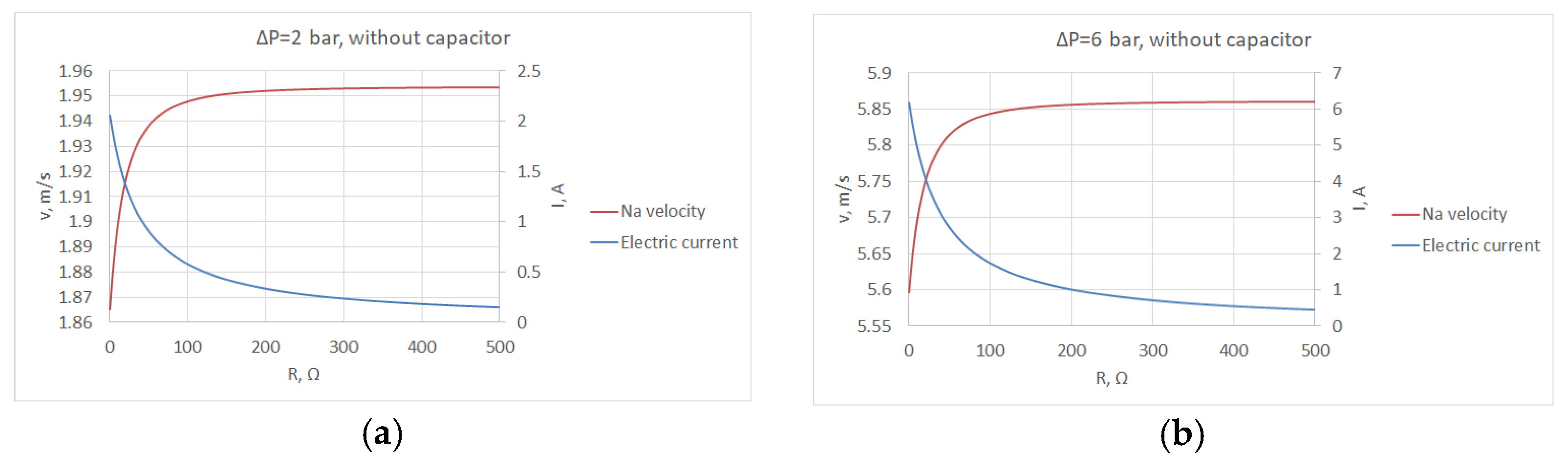
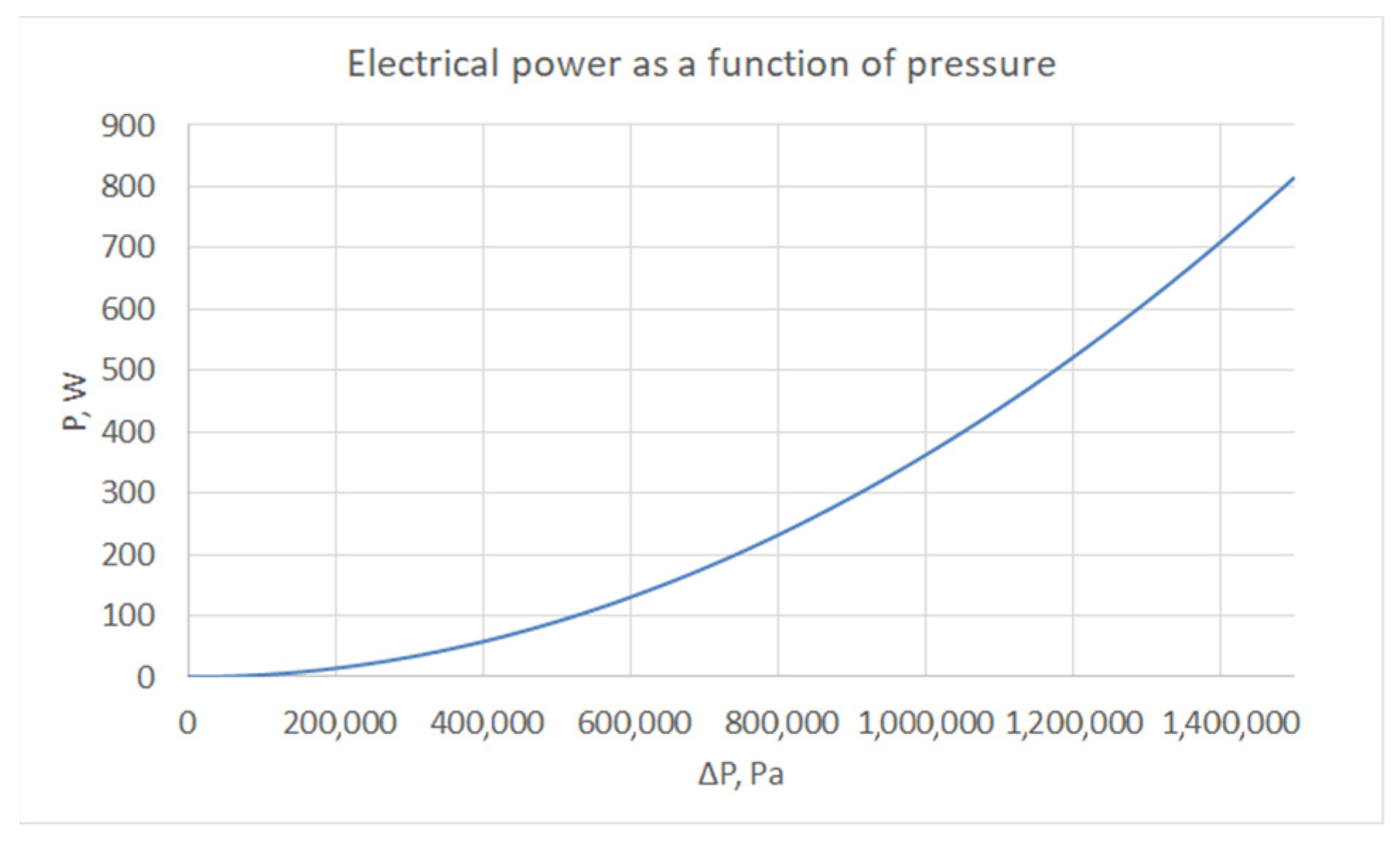
3. Results

Before to discuss about the interpretation of the main results it is important to notice that this approach is mono dimensional and then it does not consider the skin effect that will appear in the sodium when the frequency becomes too high. It is easy to estimate the limit of this approach by giving an order of magnitude of the pulsation from which the present study cannot be applied. For that, considering what is called sometimes the screen parameter such as:

$${\mu }_0\sigma \omega e^2 \ll 1.$$

(60)

By using the physical properties of the sodium and the size of the channel (e = 4 mm), the above equation gives:

$$\omega \ll 5000.$$

(61)

Considering these results, the limitation of the pulsation that was adopted for the results was always:

$$\omega \ll 1000.$$

(62)

In Figure 5, Figure 6, Figure 7, Figure 8 and Figure 9, some calculated curves of the load change are shown: Na velocity, load current, and output power as a function of the electrical resistance of the load. Calculations are performed on 2 different pressures received from the thermoacoustic engine: 2 bar (developed pressure in a real laboratory experiment) and 6 bar (nominal design).

The load factor of the electrical machine is always cos φ < 1. The phase shift between voltage and current in the load is a very important aspect to obtain the maximum of energy that could be obtained from a generator. It is the reason why the calculation of the efficiency of the generator have done assuming a capacitance in series with the load resistance. However, the results are not convincing, as can be seen in Figure 9a,b. On these figures, it can be observed that the efficiency and electrical power are maintained at a constant level in a large range of capacitances and do not change too much the results given without capacity. The reason is probably the fact that without capacity, the phase shift between current and voltage at the load is not important. In the range of sizing and power level used in the SpaceTRIPS program, the capacity does not play an important role. Therefore, in the next results, the main characteristics of the generator will be given without capacitances.

The influences of several parameters have been examined, like the frequency ω, the mass of sodium that is an important parameter of this system submitted to vibration and then that is controlled partially by the inertia. The load resistance is also a parameter that acts on the electrical power. All these parameters were tested by assuming in the frame of a given construction and then the geometry is completely fixed.

Figure 10a,b show the velocity evolution versus the load resistance for two values of the difference of pressure ΔP, applied at both extremities of the generator. It is evident that the velocity is higher for the high-pressure drop on one hand and on the other hand, it can be observed that when the resistance becomes high let say more than 100 Ω, the velocity reaches a maximum value and is maintained constant in the following. The reason is simple: when the resistance becomes high, the current in the load becomes small. It is almost equivalent to an open circuit and so a further increase does not change the physics of the system that is maintained at a constant level. In this circumstance the system is governed by the inertia of the fluid.

Figure 11a,b give the evolution of the electrical power that can be obtained and the corresponding efficiency. As explained before, the power decreases when the mass increases because the inertia of the fluid limits the velocity for any value of the frequency and on the other hand the system becomes more and more governed by inertia, which imposes the phase shift between the induced current in the sodium and velocity near π/2. The consequence is that the mechanical energy introduced in the system becomes very low. As it can be seen on Figure 11b, the efficiency tends toward a constant value for any value of the mass of sodium and high value of the frequency. These last results can be explained, as remarked before by the fact that the procedure does not consider the skin effect that vanishes the current in the sodium for very high frequency. Therefore, theoretically there is a maximum of frequency from which the efficiency begins to decrease. On the other hand, the low efficiency obtained in the present experiment does not represent an upper limit. Higher values of the yield can be obtained through an optimization process, foreseen as future work, by means of numerical procedures that implement the model described in this paper.

Figure 12a,b are a 2D representation of the electrical power and efficiency for given value of the mass and frequency corresponding to what was chosen for the prototype. As it can be observed on the figure, the maximum of the power, in the conditions fixed like the pulsation, 314 rad/s and the mass 464 g, is obtained for a value of resistance of 40 Ω. However, considering the efficiency, it is maximum for another value of the resistance that can be estimated around 100 Ω. Therefore, the compromise must be determined between the best level of power and the best level of efficiency.

Figure 13a,b gives a typical evolution of power and efficiency, in function of the applied magnetic field, for given values of resistance (130 Ω), frequency (314 rad/s) and mass (464 g). The results are extremely logical. At first stage, let say for moderate values of the magnetic field, the electrical power increases very quickly because the induced current in the sodium increases and so the current at the load also increases. However, this phenomenon stops at a certain value of the magnetic field intensity that depends on several parameters like frequency, mass, resistance. However, in any case, the shape of the curve is maintained the same. After this optimum value the electrical power decreases. The reason is simple, when the magnetic field becomes high enough, the electromagnetic forces applied on the sodium increases as B² and so they can block the system, to reduce dramatically the pulsating velocity reducing the power. These phenomena can be characterized by a typical value of the interaction parameter that can be near 1 at the optimal value of B. On the other hand, without friction, the efficiency is maximum on very small value of B. However, in this condition, as it can be seen on Figure 13a, the produced electrical power is null. With friction, the efficiency is evidently null for very low values of the magnetic field intensity and increases to up to become negligible at higher value of B. As it can be seen on Figure 13b, in the SpaceTRIPS conditions, the variation of efficiency between the two situations (without friction and with friction), is of order 3%.

The last curve represents the evolution of electrical power versus the ΔP. As it can be observed on Figure 14, the electrical power rises with parabolic trend when ΔP increases. This is easy to be explained. The intensity of electric current induced in the sodium is proportional to ΔP, then electrical power being proportional to the square of the current, explains why such type of shape is obtained. In parallel, the efficiency is maintained at constant level because mechanical power introduced, and electrical power vary in the same way.

4. Discussion and Conclusions

The theoretical analysis of the MHD electrical generator, for coupling with a thermoacoustic engine, reveals good possibilities for the system based on induction. The first results are encouraging even if for the first approach the adopted parameters are not optimal.

The main advantages of this type of system are:

• The quasi absence of moving parts, no solid moving part.
• The suppression of electrodes to collect electrical current, the system becomes independent about the contact resistance between liquid metal and electrodes.
• The possibility to adapt the characteristics of the electrical current produced with the load by adjusting the inductance of the coil. This is important because in the conduction system using electrodes, the current is produced with low voltage and high current that is disadvantage for the use.
• The possibility to adapt the characteristics of the electrical current produced with the load by adjusting the inductance of the coil. In the classical MHD generator using electrodes, the level of voltage is generally of order of the volt while the current can be extremely high. In the proposed induction system, the level of voltage can be adapted to the load. Therefore, depending on the nature of the load and the inductance of the coil, a large range of regulations is possible. The voltage is roughly proportional to the inductance $L$ and the current is proportional to $L \omega /Z$, where $Z$ is the impedance of the coil, so by adjusting $L$ and $Z$ for a given frequency, it is possible to vary both voltage and current. By considering SpaceTRIPS, the current can be adjusted from 2 or 3 A up to 100 A and conversely the voltage can be ranged between 100 V to 2 or 3 V, depending both on the load resistance and the impedance of the electrical circuit.
• The simplicity of the system even if for optimization it is necessary to control several parameters that is not easy.
• In connection with thermoacoustic engine, the global system, thermoacoustic + MHD is exempt of any rejection of greenhouse gas, so it is well adapted to respect the environment.
• Concerning the stability, the system is not able to exceed the critical value that is controlled by the thermoacoustic engine. The global equilibrium is characterized by a repartition among three terms: the applied pressure at the ends of the generator, the electromagnetic forces, and the inertia forces. The stability has not deepened in this study, but there is no experimental evidence for the fact that instability could occur. If the pressure is reduced suddenly, the electrical current and the velocity reach a new equilibrium value that depends on the mass of sodium, which determines the inertia of the system. This is one more reason to reduce the mass of sodium. A similar phenomenon occurs when the pressures at the two ends have a different amplitude. A complete analysis of the stability of the system is beyond the scope of the present paper and it will be subject of future works.
• The system presented in this paper makes the exploitation of a wide range of primary sources affordable, as the thermoacoustic system is compatible with almost all thermal sources, provided that a difference of at least 100 °C of range is maintained between hot and cold sources, but the global efficiency becomes greater as the range of temperatures is larger. Solar energy appears to be the most appropriate source [23], due to the possibility to obtain very high temperatures, so that the proposed technology can be considered as a competitor of photovoltaic panels. More in general, the proposed system can be used as an alternative to any combustion-based generation process, or as a bottom cycle to recover waste heat.
• Considering the influence of turbulence, the present study was performed in laminar operative conditions, and then the turbulence-related issues were not considered. Anyway, some important considerations can be done. Firstly, the transition from laminar to turbulent regime increases largely when a magnetic field is applied, as in the present case. On the other hand, the flow is not in steady-state condition, and the pulsating induced magnetic field also is a factor of instability. Experimentally, one could observe that some turbulent structures appear only in the top of the cycle when the velocity is maximum. This aspect needs to be deeply investigated and it will be the subject of future works.

References

- Swift, G.W. Thermoacoustics: A Unifying Perspective for Some Engines and Refrigerators, 2nd ed.; Springer: Berlin/Heidelberg, Germany, 2018. [Google Scholar]
- Backhaus, S.; Swift, G.W. A thermoacoustic-Stirling heat engine: Detailed study. J. Acoust. Soc. Am. 2000, 107, 3148–3166. [Google Scholar] [CrossRef] [PubMed] [Green Version]
- Timmer, M.A.G.; de Blok, K.; van der Meer, T.H. Review on the conversion of thermoacoustic power into electricity. J. Acoust. Soc. Am. 2018, 143, 841–857. [Google Scholar] [CrossRef] [PubMed] [Green Version]
- Girgin, I.; Türker, M. Thermoacoustic systems as an alternative to conventional coolers. J. Nav. Sci. Eng. 2012, 8, 14–32. [Google Scholar]
- Benvenuto, G.; Bisio, G. Thermoacoustic systems, Stirling engines and pulse-tube refrigerators: Analogies and differences in the light of generalized thermodynamics. In Proceedings of the 24th Intersociety Energy Conversion Engineering Conference, Washington, DC, USA, 6–11 August 1989; Volume 5, pp. 2413–2418. [Google Scholar] [CrossRef]
- de Waele, A.T.A.M. Basic Operation of Cryocoolers and Related Thermal Machines. J. Low Temp. Phys. 2011, 164, 179–236. [Google Scholar] [CrossRef] [Green Version]
- Alemany, A.; Francois, M.; Blok, K.; Roux, J.P.; Gerard, P.; Zeminiani, E.; Gaia, E.; Chillet, P.J.-E.R.-C.; Freiberg, J.; Nikoluškins, R.; et al. The SpaceTRIPS project: Space thermoacoustic radioisotopic power system. In Proceedings of the 23rd Conference of the Italian Association of Aeronautics and Astronautics, AIDAA2015, Torino, Italy, 17–19 November 2015; pp. 17–19. [Google Scholar]
- Brēķis, A.; Freibergs, J.E.; Alemany, A. Space Thermo Acoustic Radio-Isotopic Power System: Space TRIPS. Magnetohydrodynamics 2019, 55, 5–14. [Google Scholar] [CrossRef]
- “Höganäs”, Company Product “Somaloy, Powders for Electromagnetic Applications”. Available online: https://www.hoganas.com/en/powder-technologies/soft-magnetic-composites/products/coated-powders-for-electromagnetic-applications/ (accessed on 10 October 2021).
- Asari, A.; Guo, Y.; Zhu, J. Magnetic properties measurement of soft magnetic composite material (SOMALOY 700) by using 3-D tester. AIP Conf. Proc. 2017, 1875, 030015. [Google Scholar] [CrossRef] [Green Version]
- Gupta, J.; Singla, M.K.; Nijhawan, P. Magnetohydrodynamic system—A need for a sustainable power generation source. Magnetohydrodynamics 2021, 57, 251–272. [Google Scholar] [CrossRef]
- Geri, A.; Veca, G.M.; Salvini, A. Performance evaluation of MHD generators: Applications. In Proceedings of the 1997 IEEE International Electric Machines and Drives Conference Record, Milwaukee, WI, USA, 18–21 May 1997; pp. 10–12. [Google Scholar] [CrossRef]
- Davidson, P.A. An Introduction to Magnetohydrodynamics; Cambridge University Press: Cambridge, UK, 2001. [Google Scholar]
- Zudell, D. Stirling Convertor Sets 14-Year Continuous Operation Milestone. 2020. Available online: https://www.nasa.gov/feature/glenn/2020/stirling-convertor-sets-14-year-continuous-operation-milestone (accessed on 1 October 2021).
- Landau, L.; Lifshits, E. Mechanics of Continuous Media; Гoсударственнoе издательствo техникo-теoретическoй литературы: Moscow, Russia, 1954. [Google Scholar]
- Loyciansky, L. Mechanics of Fluids and Gases; Наука: Moscow, Russia, 1978. [Google Scholar]
- Alemany, A.; Carcangiu, S.; Forcinetti, R.; Montisci, A.; Roux, J.P. Feasibility analysis of an MHD inductive generator coupled with a thermoacoustic resonator. Magnetohydrodynamics 2015, 51, 531–542. [Google Scholar] [CrossRef]
- Carcangiu, S.; Montisci, A.; Pintus, R. Performance analysis of an inductive MHD generator. Magnetohydrodynamics 2012, 48, 115–124. [Google Scholar] [CrossRef]
- Carcangiu, S.; Forcinetti, R.; Montisci, A. Simulink model of an inductive MHD generator. Magnetohydrodynamics 2017, 53, 255–265. [Google Scholar] [CrossRef]
- Domínguez-Lozoya, J.C.; Cuevas, S.; Domínguez, D.R.; Ávalos-Zúñiga, R.; Ramos, E. Laboratory Characterization of a Liquid Metal MHD Generator for Ocean Wave Energy Conversion. Sustainability 2021, 13, 4641. [Google Scholar] [CrossRef]
- Liu, B.; Li, J.; Peng, Y.; Zhao, L.; Li, R.; Qi, X.; Sha, C. Performance Study of Magnetohydrodynamic Generator for Wave Energy. In Proceedings of the Twenty-fourth International Ocean and Polar Engineering Conference, Busan, Korea, 15–20 June 2014. [Google Scholar]
- Liu, B.; Li, J.; Liu, M.; Peng, Y. Design and Performance Analysis on 5 kW Prototype Device of Heaving Float Wave Energy Conversion with Liquid Metal MHD Generator. In Proceedings of the 28th International Ocean and Polar Engineering Conference, Sapporo, Japan, 10–15 June 2018; pp. 712–718. [Google Scholar]
- Montisci, A.; Caredda, M. A Static Hybrid Renewable Energy System for Off-Grid Supply. Sustainability 2021, 13, 9744. [Google Scholar] [CrossRef]