
A Novel Stacked Long Short-Term Memory Approach of Deep Learning for Streamflow Simulation

 ,
,  , ,
, ,  and
and 
Abstract
:1. Introduction
2. Methodology
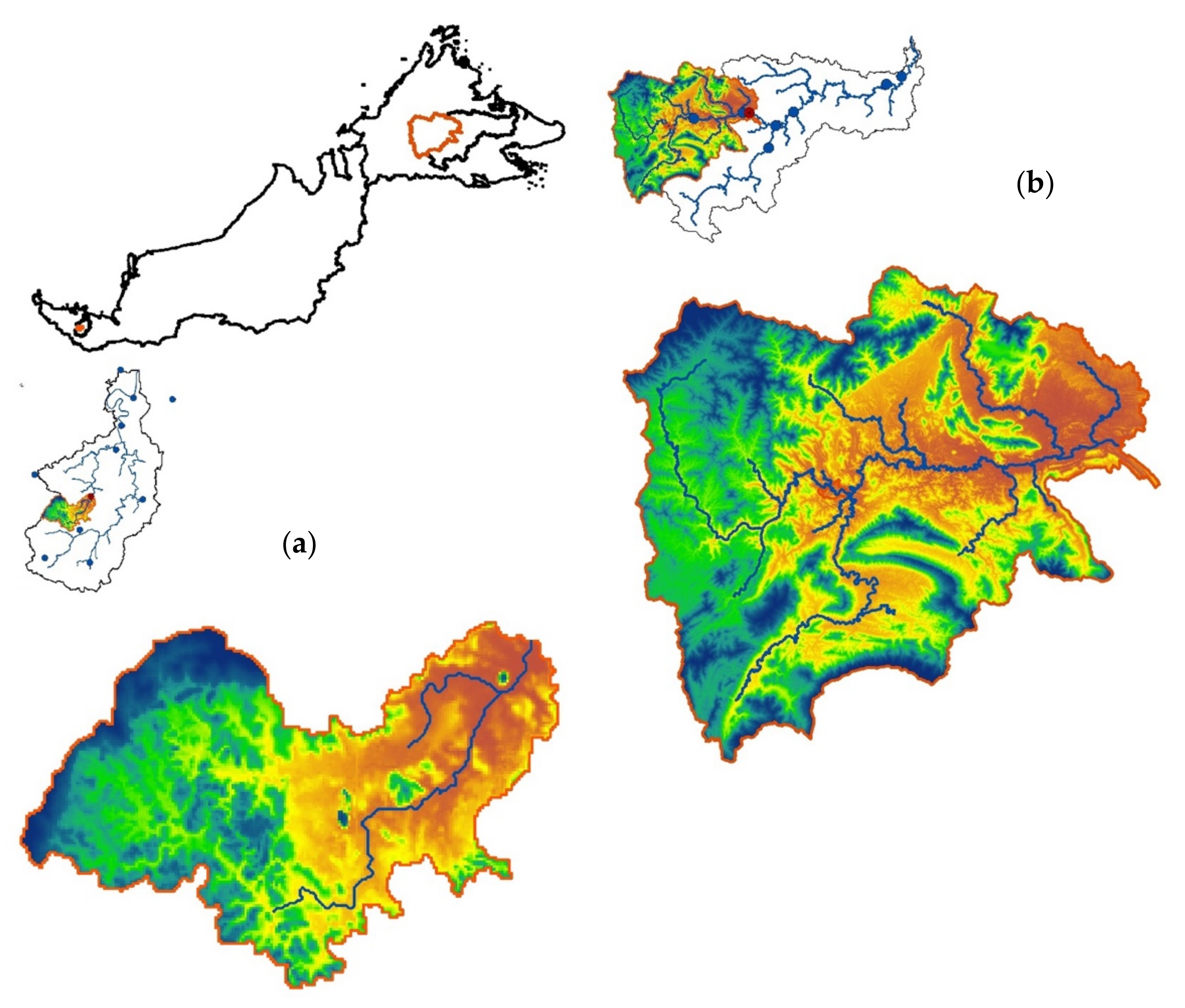
2.1. Study Area
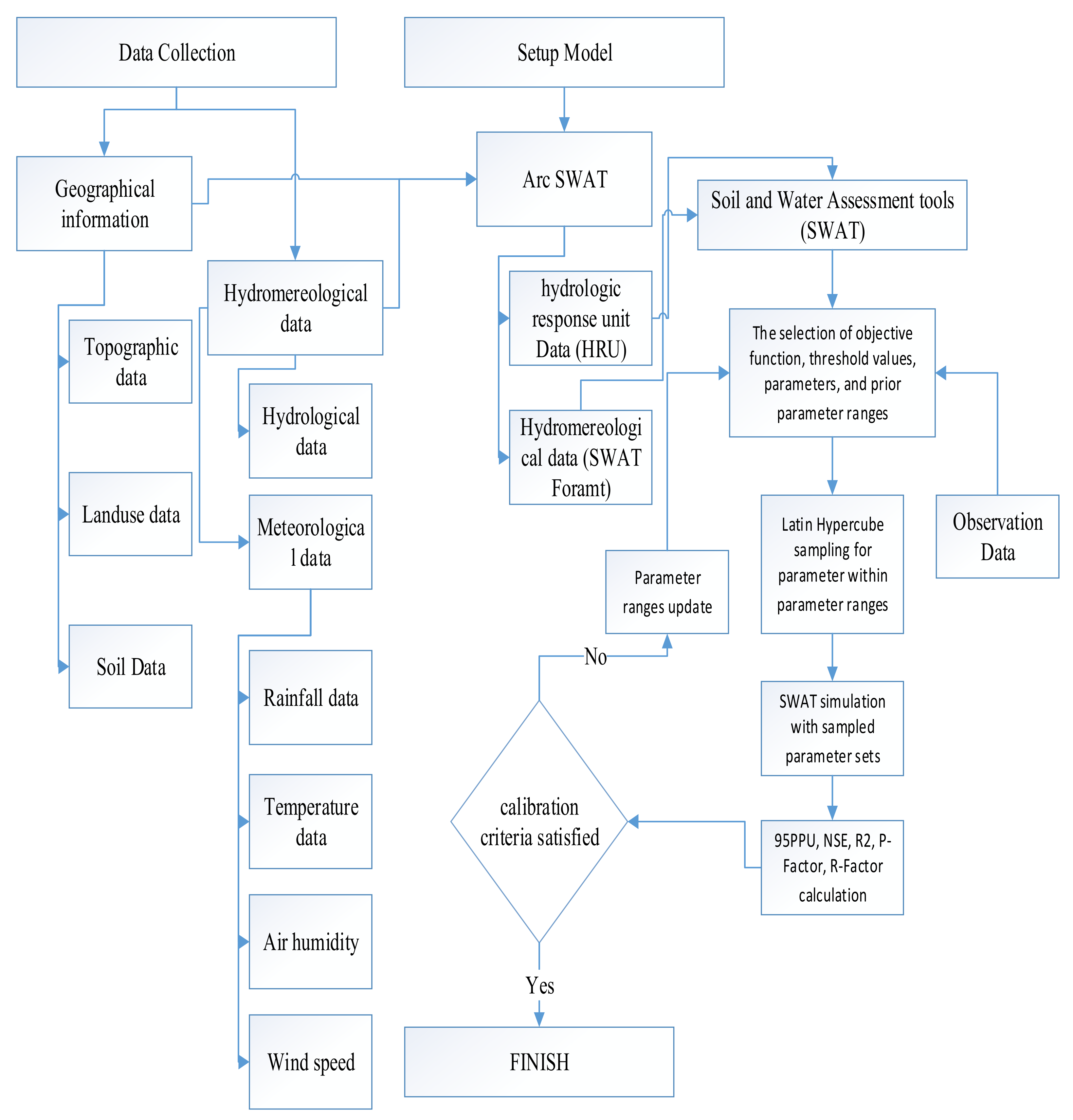
2.2. Distributed Modelling—The SWAT Hydrological Model
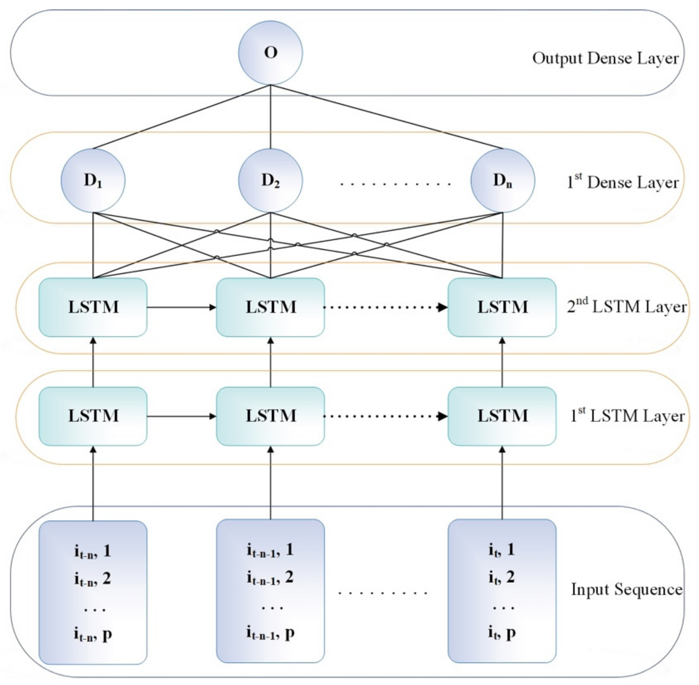
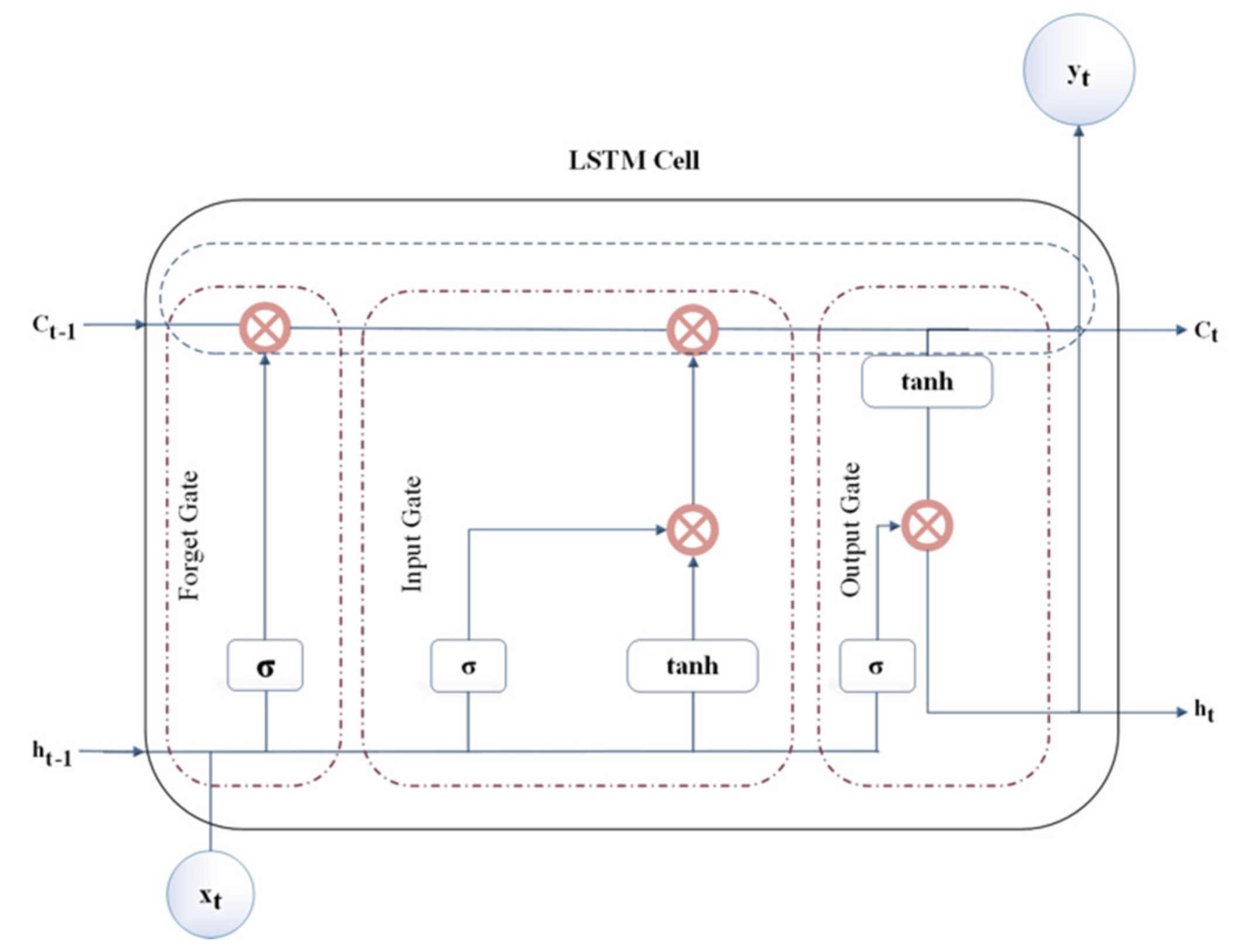
2.3. Data-Driven Models—The Long Short-Term Memory Model (LSTM)
2.4. SLSTM Setup
3. Results and Discussion
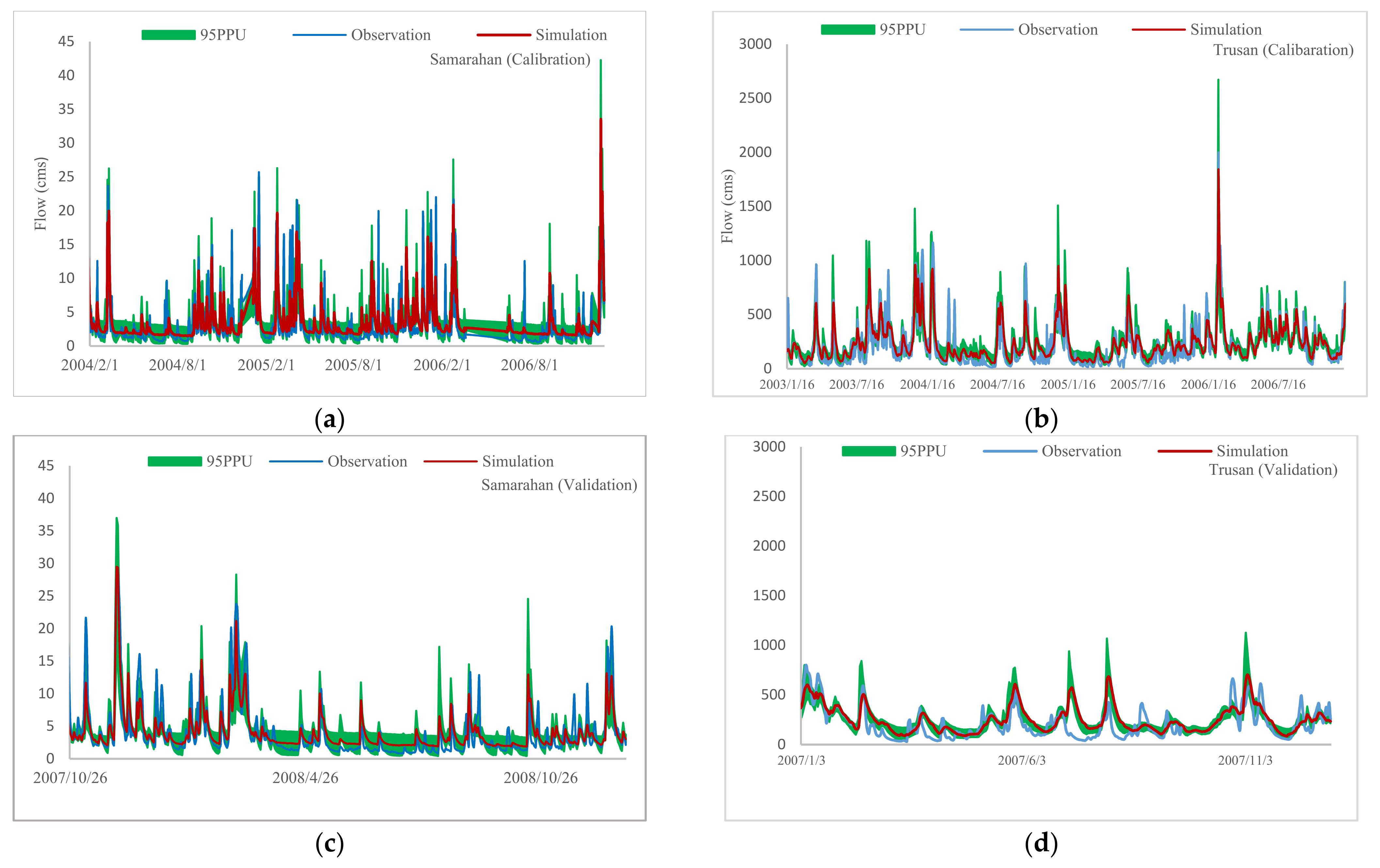
3.1. The SWAT Performance Evaluation
3.2. The SLSTM Performance Evaluation
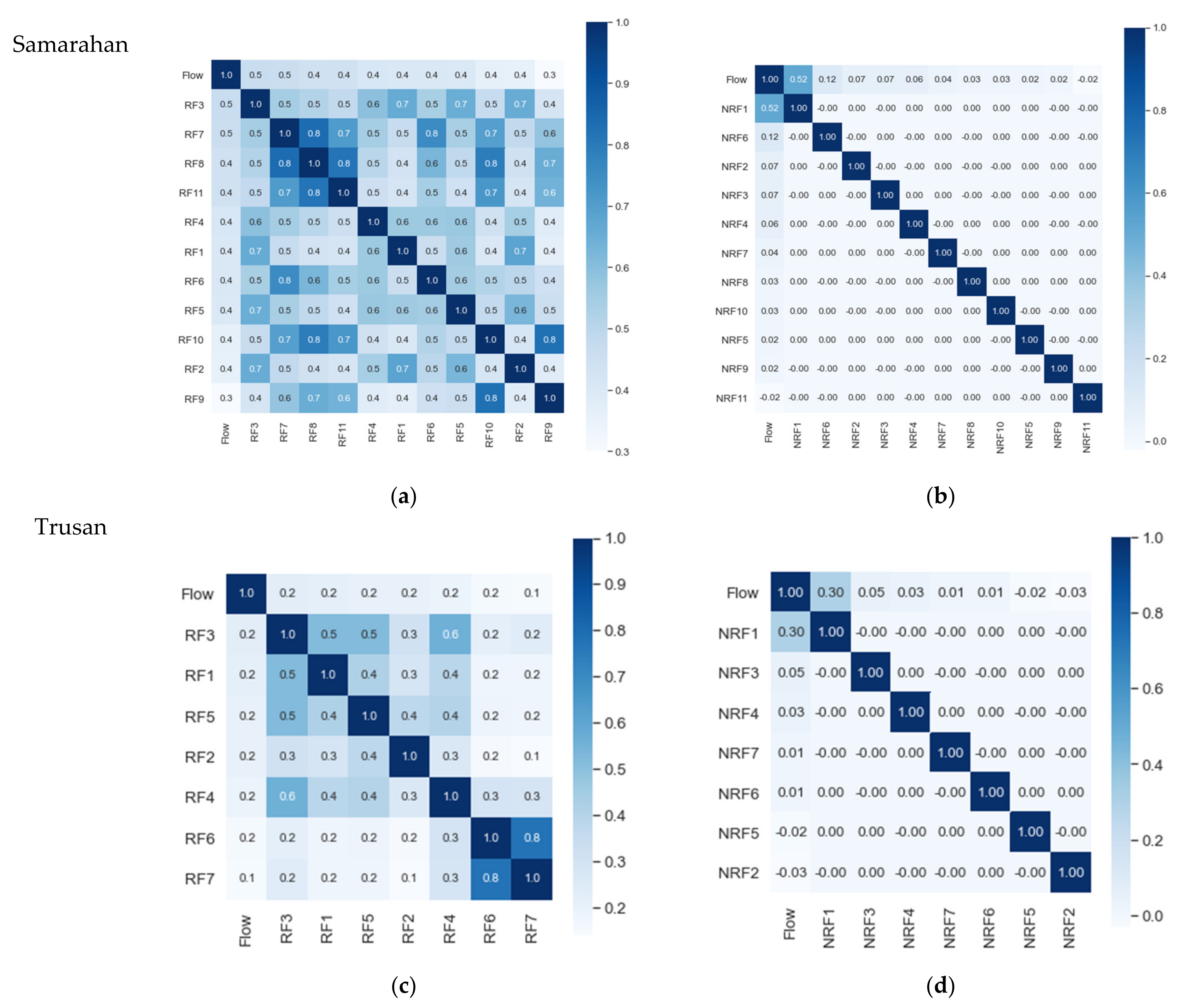
3.2.1. Data Preprocessing
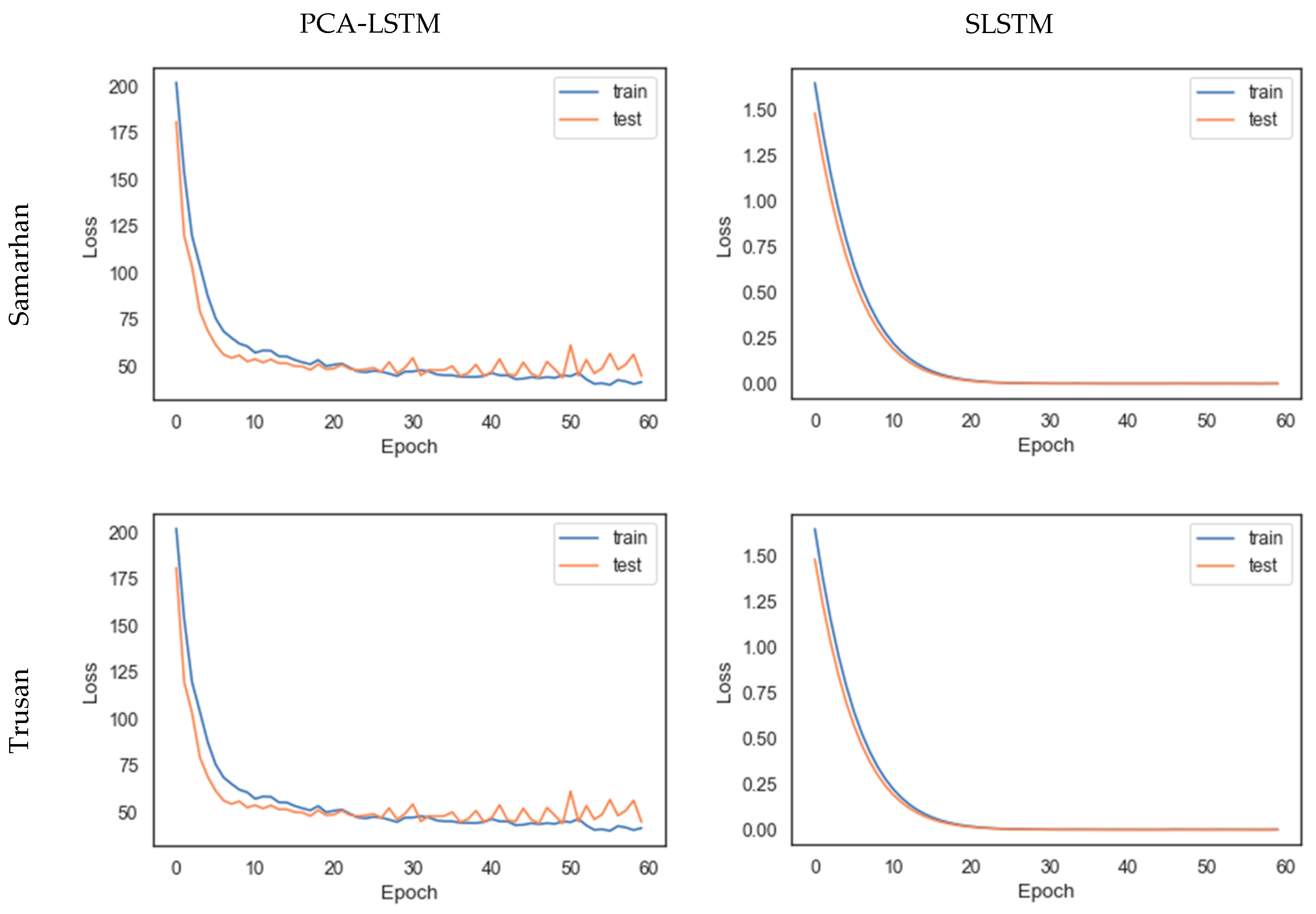
3.2.2. Tuning the Model
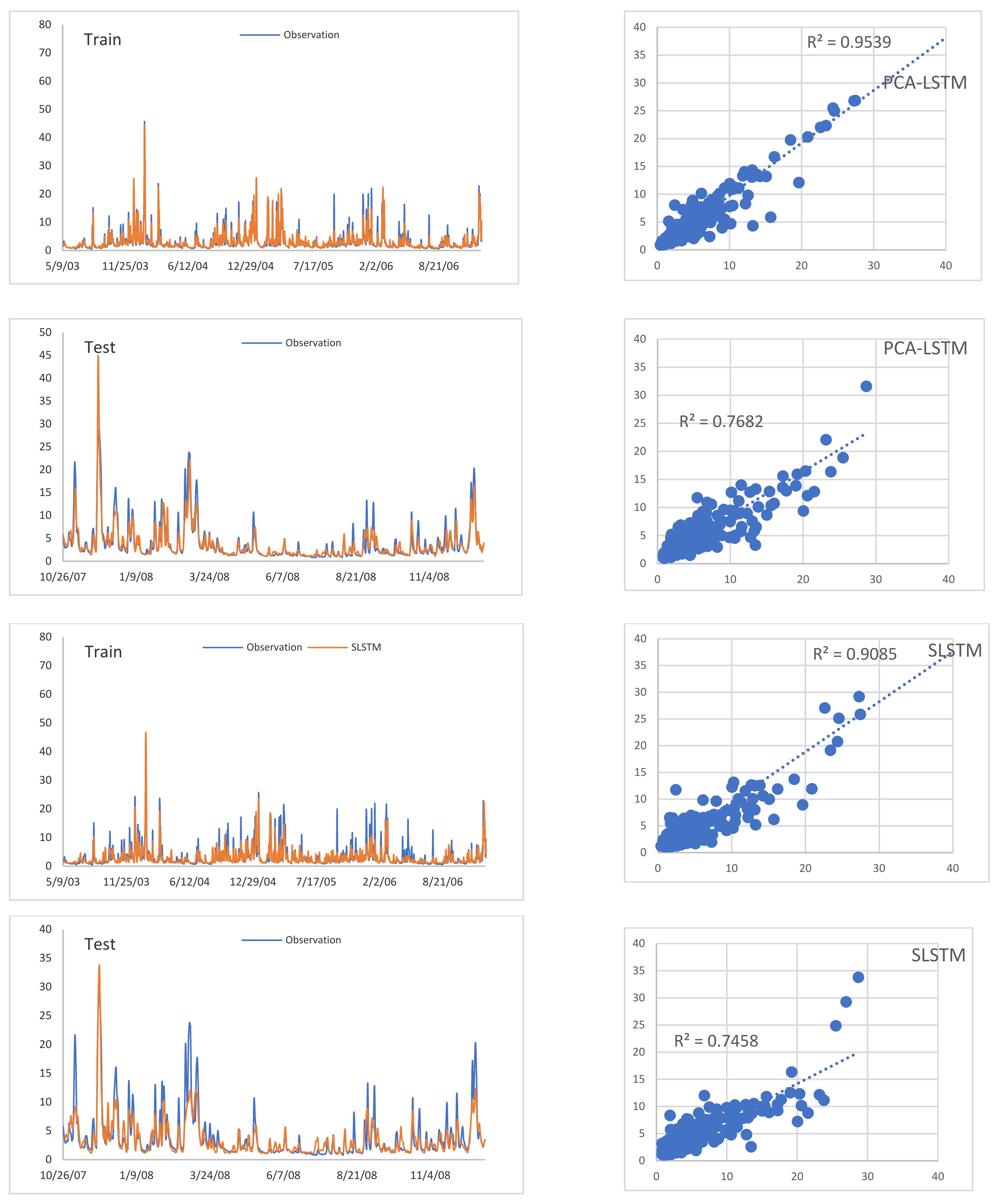
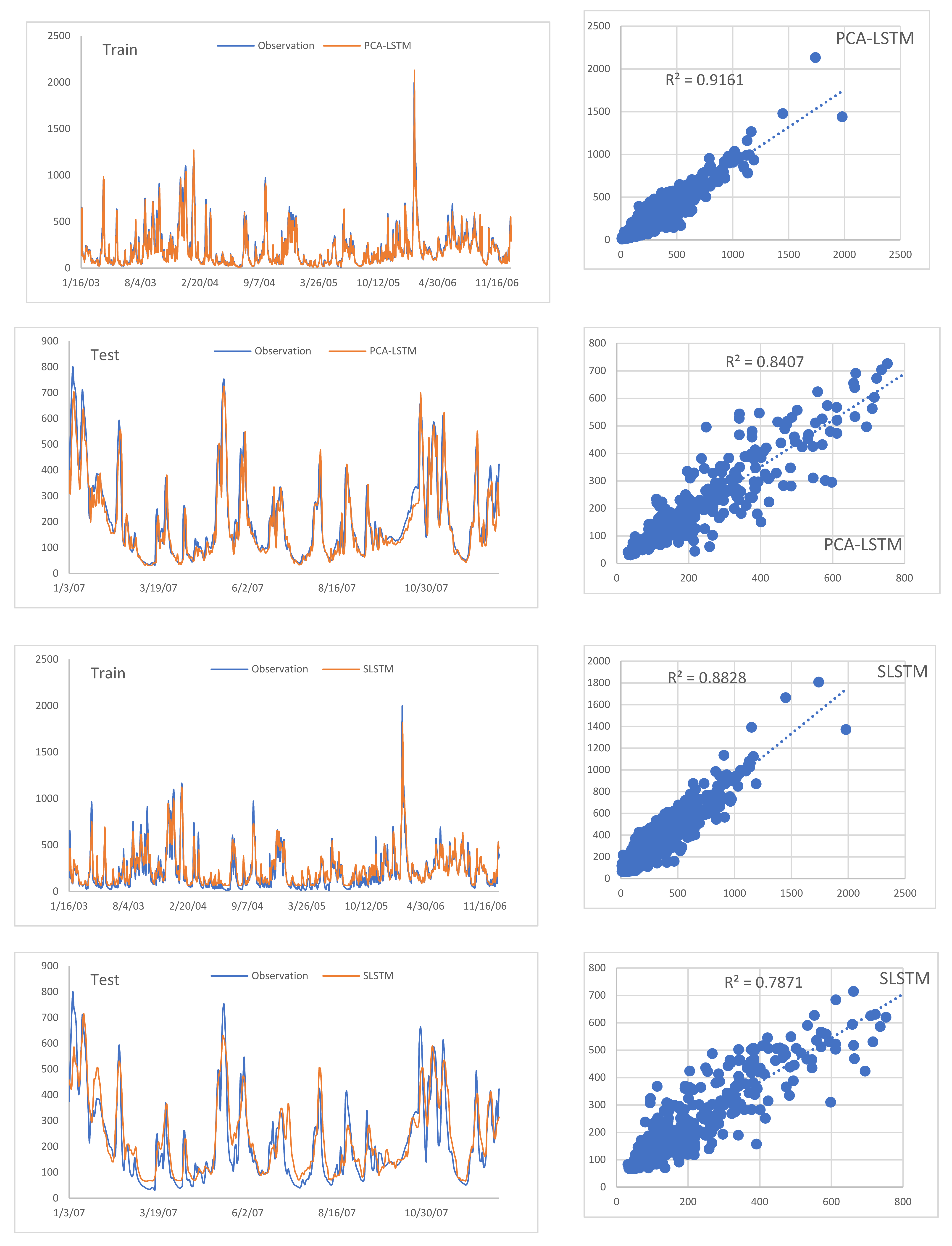
3.2.3. The Models Performance Comparison
3.3. Conclusions
Author Contributions
Funding
Institutional Review Board Statement
Informed Consent Statement
Data Availability Statement
Conflicts of Interest
References
- Mirzaei, M.; Huang, Y.F.; El-Shafie, A.; Chimeh, T.; Lee, J.; Vaizadeh, N.; Adamowski, J.; Valizadeh, N. Uncertainty analysis for extreme flood events in a semi-arid region. Nat. Hazards 2015, 78, 1947–1960. [Google Scholar] [CrossRef]
- Ravazzani, G.; Valle, F.D.; Gaudard, L.; Mendlik, T.; Gobiet, A.; Mancini, M. Assessing Climate Impacts on Hydropower Production: The Case of the Toce River Basin. Climate 2016, 4, 16. [Google Scholar] [CrossRef]
- Ramireddygari, S.; Sophocleous, M.; Koelliker, J.; Perkins, S.; Govindaraju, R. Development and application of a comprehensive simulation model to evaluate impacts of watershed structures and irrigation water use on streamflow and groundwater: The case of Wet Walnut Creek Watershed, Kansas, USA. J. Hydrol. 2000, 236, 223–246. [Google Scholar] [CrossRef]
- Galavi, H.; Mirzaei, M.; Shul, L.T.; Valizadeh, N.; Shui, L.T. Klang River-level forecasting using ARIMA and ANFIS models. J. Am. Water Work. Assoc. 2013, 105, E496–E506. [Google Scholar] [CrossRef]
- Valizadeh, N.; El-Shafie, A.; Mirzaei, M.; Galavi, H.; Mukhlisin, M.; Jaafar, O. Accuracy Enhancement for Forecasting Water Levels of Reservoirs and River Streams Using a Multiple-Input-Pattern Fuzzification Approach. Sci. World J. 2014, 2014, 1–9. [Google Scholar] [CrossRef]
- Rujner, H.; Leonhardt, G.; Marsalek, J.; Viklander, M. High-resolution modelling of the grass swale response to runoff inflows with Mike SHE. J. Hydrol. 2018, 562, 411–422. [Google Scholar] [CrossRef]
- Sonnenborg, T.O.; Christiansen, J.R.; Pang, B.; Bruge, A.; Stisen, S.; Gundersen, P. Analyzing the hydrological impact of afforestation and tree species in two catchments with contrasting soil properties using the spatially distributed model MIKE SHE SWET. Agric. For. Meteorol. 2017, 239, 118–133. [Google Scholar] [CrossRef]
- Metcalfe, P.; Beven, K.; Freer, J. Dynamic TOPMODEL: A new implementation in R and its sensitivity to time and space steps. Environ. Model. Softw. 2015, 72, 155–172. [Google Scholar] [CrossRef] [Green Version]
- Amirabadizadeh, M.; Ghazali, A.H.; Huang, Y.F.; Wayayok, A. Assessment of impacts of future climate change on water resources of the Hulu Langat basin using the swat model. Water Harvest. Res. 2017, 2, 13–29. [Google Scholar]
- Salimirad, H.; Dehvari, A.; Galavi, H.; Ebrahimian, M. Identification and Uncertainty Analysis of Sensitive Parameter of SWAT model in Kardeh Streamflow Simulation. Iran Water Resour. Res. 2020, 16, 212–221. [Google Scholar]
- Mirzaei, M.; Galavi, H.; Faghih, M.; Huang, Y.F.; Lee, T.S.; El-Shafie, A. Model calibration and uncertainty analysis of runoff in the Zayanderood River basin using generalized likelihood uncertainty estimation (GLUE) method. J. Water Supply Res. Technol. 2013, 62, 309–320. [Google Scholar] [CrossRef]
- Mirzaei, M.; Huang, Y.F.; Lee, T.S.; El-Shafie, A.; Ghazali, A.H. Quantifying uncertainties associated with depth duration frequency curves. Nat. Hazards 2014, 71, 1227–1239. [Google Scholar] [CrossRef]
- Galavi, H.; Mirzaei, M. Analyzing Uncertainty Drivers of Climate Change Impact Studies in Tropical and Arid Climates. Water Resour. Manag. 2020, 34, 2097–2109. [Google Scholar] [CrossRef]
- Gassman, P.W.; Reyes, M.R.; Green, C.H.; Arnold, J.G. The Soil and Water Assessment Tool: Historical Development, Applications, and Future Research Directions. Am. Soc. Agric. Biol. Eng. 2007, 50, 1211–1250. [Google Scholar] [CrossRef] [Green Version]
- Srinivasan, R.; Ramanarayanan, T.S.; Arnold, J.G.; Bednarz, S.T. LARGE AREA HYDROLOGIC MODELING AND ASSESSMENT PART II: MODEL APPLICATION. JAWRA J. Am. Water Resour. Assoc. 1998, 34, 91–101. [Google Scholar] [CrossRef]
- Amini-Zad, A.; Galavi, H.; MohammadRezaPoor, O. Hydrological Modeling of Pishin Dam Watershed Using SWAT. Development and Applications of Soil and Water Assessment Tool (SWAT) in WAter Resources Management. 2018, pp. 26–30. Available online: https://civilica.com/doc/820016/ (accessed on 28 November 2021).
- Galavi, H.; Lee, T.S. Neuro-fuzzy modelling and forecasting in water resources. Sci. Res. Essays 2012, 7, 2112–2121. [Google Scholar] [CrossRef]
- Valizadeh, N.; Mirzaei, M.; Allawi, M.F.; Afan, H.A.; Mohd, N.S.; Hussain, A.; El-Shafie, A. Artificial intelligence and geo-statistical models for stream-flow forecasting in ungauged stations: State of the art. Nat. Hazards 2017, 86, 1377–1392. [Google Scholar] [CrossRef]
- Mohsenzadeh Karimi, S.; Karimi, S.; Poorrajabali, M. Forecasting monthly streamflows using heuristic models. ISH J. Hydraul. Eng. 2021, 27, 73–78. [Google Scholar] [CrossRef]
- Pakdaman, M.; Falamarzi, Y.; Babaeian, I.; Javanshiri, Z. Post-processing of the North American multi-model ensemble for monthly forecast of precipitation based on neural network models. Theor. Appl. Clim. 2020, 141, 405–417. [Google Scholar] [CrossRef]
- Palizdan, N.; Falamarzi, Y.; Huang, Y.F.; Lee, T.S. Precipitation trend analysis using discrete wavelet transform at the Langat River Basin, Selangor, Malaysia. Stoch. Environ. Res. Risk Assess. 2017, 31, 853–877. [Google Scholar] [CrossRef]
- Nourani, V.; Komasi, M. A geomorphology-based ANFIS model for multi-station modeling of rainfall-runoff process. J. Hydrol. 2013, 490, 41–55. [Google Scholar] [CrossRef]
- Shortridge, J.E.; Guikema, S.D.; Zaitchik, B.F. Machine learning methods for empirical streamflow simulation: A comparison of model accuracy, interpretability, and uncertainty in seasonal watersheds. Hydrol. Earth Syst. Sci. 2016, 20, 2611–2628. [Google Scholar] [CrossRef] [Green Version]
- Sun, A.; Wang, D.; Xu, X. Monthly streamflow forecasting using Gaussian Process Regression. J. Hydrol. 2014, 511, 72–81. [Google Scholar] [CrossRef]
- Hochreiter, S.; Schmidhuber, J. Long Short-Term Memory. Neural Comput. 1997, 9, 1735–1780. [Google Scholar] [CrossRef]
- Mouatadid, S.; Adamowski, J.F.; Tiwari, M.K.; Quilty, J.M. Coupling the maximum overlap discrete wavelet transform and long short-term memory networks for irrigation flow forecasting. Agric. Water Manag. 2019, 219, 72–85. [Google Scholar] [CrossRef]
- Kratzert, F.; Klotz, D.; Brenner, C.; Schulz, K.; Herrnegger, M. Rainfall-runoff modelling using Long Short-Term Memory (LSTM) networks. Hydrol. Earth Syst. Sci. 2018, 22, 6005–6022. [Google Scholar] [CrossRef] [Green Version]
- Ni, L.; Wang, D.; Singh, V.P.; Wu, J.; Wang, Y.; Tao, Y.; Zhang, J. Streamflow and rainfall forecasting by two long short-term memory-based models. J. Hydrol. 2020, 583, 124296. [Google Scholar] [CrossRef]
- Hu, Z.; Liu, W.; Bian, J.; Liu, X.; Liu, T.-Y. Listening to Chaotic Whispers. In Proceedings of the Eleventh ACM International Conference on Web Search and Data Mining; ACM Press: New York, NY, USA, 2018; pp. 261–269. [Google Scholar] [CrossRef]
- Le, X.-H.; Ho, H.V.; Lee, G.; Jung, S. Application of Long Short-Term Memory (LSTM) Neural Network for Flood Forecasting. Water 2019, 11, 1387. [Google Scholar] [CrossRef] [Green Version]
- Arnold, J.G.; Srinivasan, R.; Muttiah, R.S.; Williams, J.R. Large area hydrologic modeling and assessment part I: Model development. JAWRA J. Am. Water Resour. Assoc. 1998, 34, 73–89. [Google Scholar] [CrossRef]


| Station | Type | Name | Longitude | Latitude | |
|---|---|---|---|---|---|
| Trusan | Ulu Kuamut | Rainfall | RF1 | 117.44 | 5.08 |
| Tongod | Rainfall | RF2 | 116.97 | 5.27 | |
| Kuamut Met | Rainfall | RF3 | 117.49 | 5.22 | |
| Balat | Rainfall | RF4 | 117.6 | 5.31 | |
| Tangkulap | Rainfall | RF5 | 117.28 | 5.3 | |
| Bilit | Rainfall | RF6 | 118.19 | 5.49 | |
| Sukau | Rainfall | RF7 | 118.28 | 5.53 | |
| Milian | StreamFlow | SF1 | 117.32 | 5.3 | |
| Samarahan | Gayu | Rainfall | RF1 | 110.34 | 1.22 |
| Plaman Nyabet | Rainfall | RF2 | 110.44 | 1.21 | |
| Dragon School | Rainfall | RF3 | 110.42 | 1.28 | |
| Semongok | Rainfall | RF4 | 110.32 | 1.39 | |
| Samarahan Estate | Rainfall | RF5 | 110.55 | 1.39 | |
| Paya Paloh | Rainfall | RF6 | 110.49 | 1.34 | |
| Baru | Rainfall | RF7 | 110.5 | 1.44 | |
| Ketup | Rainfall | RF8 | 110.53 | 1.49 | |
| Semera | Rainfall | RF9 | 110.67 | 1.55 | |
| Asa Jaya | Rainfall | RF10 | 110.61 | 1.55 | |
| Similang | Rainfall | RF11 | 110.5 | 1.61 | |
| Batu Gong | StreamFlow | SF1 | 110.44 | 1.35 |
| Parameter | Definition | Lower Band | Upper Band | Adjusted Value (Trusan) | Adjusted Value (Samarahan) |
|---|---|---|---|---|---|
| R__RCHRG_DP.gw | Deep aquifer percolation | −0.2 | 0.1 | −0.14555 | 0.0529 |
| R__SOL_BD(..).sol | Moist bulk density | 0 | 0.4 | 0.2518 | 0.0202 |
| V__TLAPS.sub | Temperature lapse rate | −8 | −5 | −7.1495 | −7.7434 |
| V__PLAPS.sub | Precipitation lapse rate | 100 | 300 | 105.5 | 110 |
| R__SLSUBBSN.hru | Slope sub-basin | −0.1 | 0.3 | −0.0639 | 0.234 |
| R__SHALLST.gw | Initial depth of water in the shallow aquifer | −0.3 | 0.1 | −0.2469 | 0.046 |
| R__GWQMN.gw | Threshold depth of water in the shallow aquifer required for return flow to occur | −0.2 | 0.4 | 0.3 | 0.15 |
| V__CH_N2.rte | Manning’s “n” value for the main channel | 0.1 | 0.4 | 0.21145 | 0.3216 |
| R__CN2.mgt | Curve number for moisture condition II | −0.15 | 0.15 | −0.13395 | −0.0549 |
| R__SOL_AWC(..).sol | Available Water Capacity is calculated as the difference between field capacity at the wilting point | 0 | 0.6 | 0.1515 | 0.5542 |
| R__SOL_K(..).sol | Saturated hydraulic conductivity | −0.1 | 0.3 | 0.0927 | 0.2356 |
| R__OV_N.hru | Manning’s N | 5 | 9.5 | 6.9 | 9.1 |
| V__GW_DELAY.gw | Groundwater delay | 200 | 500 | 218.925003 | 491.684204 |
| R__GW_REVAP.gw | Groundwater ‘‘revap’’ coefficient | −0.2 | 0 | −0.1895 | −0.1962 |
| V__REVAPMN.gw | Threshold depth of water for ‘‘revap” to occur’ | 600 | 1200 | 1039.300049 | 804.144592 |
| R__ALPHA_BNK.rte | Baseflow alpha factor for bank storage | 0 | 0.2 | 0.1895 | 0.0878 |
| R__ALPHA_BF.gw | Base flow alpha factor | 0 | 0.6 | 0.105875 | 0.5973 |
| R__CH_K2.rte | Effective hydraulic conductivity in main channel alluvium | −0.1 | 0.2 | 0.02495 | −0.0565 |
| V__EPCO.hru | Plant uptake compensation factor | 0.8 | 1 | 0.8455 | 1.0705 |
| V__ESCO.hru | Soil evaporation compensation factor | 0.1 | 0.3 | 0.2485 | 0.2834 |
| Samarahan | Trusan | |||||||||||
|---|---|---|---|---|---|---|---|---|---|---|---|---|
| R2 | RMSE (cms) | NSE | R2 | RMSE | NSE | |||||||
| Train | Test | Train | Test | Train | Test | Train | Test | Train | Test | Train | Test | |
| PCA-SLSTM | 0.95 | 0.76 | 1.47 | 2.09 | 0.89 | 0.76 | 0.91 | 0.84 | 73 | 68 | 0.8 | 0.82 |
| SLSTM | 0.9 | 0.74 | 2.07 | 2.26 | 0.78 | 0.72 | 0.88 | 0.78 | 88 | 77 | 0.86 | 0.77 |
| SWAT | 0.5 | 0.67 | 2.8 | 2.53 | 0.49 | 0.66 | 0.65 | 0.42 | 157.3 | 132.5 | 0.45 | 0.34 |
Publisher’s Note: MDPI stays neutral with regard to jurisdictional claims in published maps and institutional affiliations. |
© 2021 by the authors. Licensee MDPI, Basel, Switzerland. This article is an open access article distributed under the terms and conditions of the Creative Commons Attribution (CC BY) license (https://creativecommons.org/licenses/by/4.0/).
Share and Cite
Mirzaei, M.; Yu, H.; Dehghani, A.; Galavi, H.; Shokri, V.; Mohsenzadeh Karimi, S.; Sookhak, M. A Novel Stacked Long Short-Term Memory Approach of Deep Learning for Streamflow Simulation. Sustainability 2021, 13, 13384. https://doi.org/10.3390/su132313384
Mirzaei M, Yu H, Dehghani A, Galavi H, Shokri V, Mohsenzadeh Karimi S, Sookhak M. A Novel Stacked Long Short-Term Memory Approach of Deep Learning for Streamflow Simulation. Sustainability. 2021; 13(23):13384. https://doi.org/10.3390/su132313384
Chicago/Turabian StyleMirzaei, Majid, Haoxuan Yu, Adnan Dehghani, Hadi Galavi, Vahid Shokri, Sahar Mohsenzadeh Karimi, and Mehdi Sookhak. 2021. "A Novel Stacked Long Short-Term Memory Approach of Deep Learning for Streamflow Simulation" Sustainability 13, no. 23: 13384. https://doi.org/10.3390/su132313384
APA StyleMirzaei, M., Yu, H., Dehghani, A., Galavi, H., Shokri, V., Mohsenzadeh Karimi, S., & Sookhak, M. (2021). A Novel Stacked Long Short-Term Memory Approach of Deep Learning for Streamflow Simulation. Sustainability, 13(23), 13384. https://doi.org/10.3390/su132313384