Peak of SO₂ Emissions Embodied in International Trade: Patterns, Drivers and Implications

Abstract

International trade links countries consuming goods and services to those where products and related SO₂ pollution are produced, thereby affecting national mitigation responsibilities. This study combined accounting and decomposition techniques to investigate the patterns and drivers of SO₂ emissions embodied in international trade from 1995 to 2015 and quantified the contribution of each country or region on the production and consumption sides. The global embodied emissions increased at an accelerated rate before the global financial crisis and peaked at 51.3 Mt in 2008, followed by a fluctuating decline from 2008 to 2015. Spatially, the transfers of SO₂ emissions tended to flow from developed countries to less developed ones, but the trend has weakened after the financial crisis. Our decomposition analysis suggests that the energy and production system transitions and the slowdown in international trade jointly accounted for the peak and decline in emissions. Our contribution analysis indicates that developing economies have contributed to decreased emissions due to their recent efforts in production technology upgrading, energy efficiency improvement and energy structure optimization. The influence of developed economies on emissions decreased due to their reduced dependency on imports. Targeted policy methods are provided from the production and consumption perspectives for developing and developed economies, respectively.

1. Introduction

SO_X (including sulfur monoxide and sulfur dioxide) are the world’s second largest GHG and have maintained an increasing trend, posing a serious threat to regional ecological, environmental and human health. Sulfur dioxide (SO₂) is known to cause serious environmental issues, such as acid rain and fog-haze, and frequent SO₂ exposure can induce cardiovascular and respiratory diseases, causing serious damage to human health [1]. Moreover, due to the growing population and accelerated urbanization in developing countries, as well as the accompanying improvement of living standards, the resulting pollution emissions (e.g., carbon dioxides, SO₂ and nitrogen oxides) from these regions have also grown at an alarming rate [2]. However, in the era of economic globalization, production in a country is not only to meet its own needs but also to meet the demand of the export market [3]. Thus, international trade separates countries consuming products from countries where products and related environmental pollutants are made. Actually, not only the knowledge where the pollution is produced but also the understanding where the products related to the pollution are eventually consumed would affect the effectiveness of pollution reduction efforts [4]. Ignoring the impacts of trade on regional emissions could result in a misunderstanding of the determinants behind regional pollution and misleading regional emission reduction policies [5]. Therefore, it is an urgent issue to investigate the patterns and drivers of the SO₂ emissions embodied in international trade so as to provide information for designing fair and effective mitigation policies from both the production and consumption perspectives.

2. Literature Review

The relationship between trade and the environment has been viewed largely through the lens of comparative advantage [6]. Pollution embodied in trade (PET) is an environmental outcome of the spatial mismatch between production and final consumption in the context of trade liberalization [7]. The interaction between inter-industry trade liberalization and environmental quality has been examined extensively in the literature [8]. A strand of the literature maps the flows of PET, offering strong evidence on the imbalance of PET between developed and developing economies [9]. On the other hand, intra-industry trade rejects that products are produced under identical technical conditions due to greater varieties of intermediate and final goods [10]. Since pollution emissions are subject to the technical conditions of production, the intra-industry trade will trigger the flows of PET naturally. However, Leitão et al. found that agricultural intra-industry trade was negatively correlated with CO₂ emissions in European Union [11], and trade intensity contributed to environmental improvements in Portugal [12], confirming the less pollutant hypothesis. Thus, it plays an essential part in environment protection and trade promotion to properly deal with the relationship between trade and the environment.

In this regard, the multi-regional input–output analysis (MRIO; Leontief [13]) is a popular tool that has been widely applied to estimate emissions embodied in trade [14]. More specifically, the existing studies mainly focus on international transfers between countries [11,15], intranational transfers between provinces [16,17] or industries [18,19]. For example, Feng et al. [20] firstly employed the MRIO method to estimate the carbon emissions embodied in goods and services traded between provincial regions in China and internationally. Moreover, it was revealed that considerable amounts of pollutant emissions were produced for products traded domestically [21] or internationally [22,23]. According to the findings of Arce et al. [24], more than 20% of the global CO₂ emissions were from products that were traded across country borders. Moreover, Oita et al. [25] revealed that the amount of nitrogen emissions embodied in international trade accounted for nearly 25% of the global emissions.

As for the SO₂ emissions embodied in trade, the existing studies can be mainly divided into three categories. The first category focuses on the inter-regional SO₂ transfers within the borders of a country [17,26]. In these studies, a common finding was revealed that about 20–30% of China’s SO₂ emissions were embodied in the commodities trade between the provinces and SO₂ pollution tended to transfer from the coastal rich provinces to inner-land undeveloped regions [27,28]. The second category focuses on the embodied SO₂ emissions in the export of a country or region [29,30]. For example, Chuai et al. [30] employed the Eora input–output model to calculate the SO₂ emissions embodied in China’s imports and exports and found that the exports generated more SO₂ emissions than the imports. The third category focuses on the SO₂ transfers between countries via international trade [31]. Zhong et al. [32] estimated the sulfur oxides emissions embodied in international trade from 1995 to 2011 and found that the embodied emissions tended to flow from developed economies, such as the USA, to undeveloped ones, such as China. However, to date, there have been no studies on the SO₂ emissions embodied in international trade covering the years beyond 2012, which results in the failure to present the longer-term trends in embodied SO₂ emissions and reveal some interesting findings (e.g., the peak and decline in global embodied SO₂ emissions).

The existing studies have unveiled the invisible transfers of SO₂ emissions embodied in interregional trade. However, it is not sufficient for laying an informational foundation for the guidance of designing fair and reasonable mitigation policies, which requires not only the understanding of the SO₂ flows themselves but also their underlying determinants. In this regard, both index decomposition analysis (IDA) and structural decomposition analysis (SDA) are popular techniques in quantifying the driving factors of a dependent variable. The two methods have their own advantages. More specifically, IDA has a lower requirement for data and has more ease of application, while SDA enables us to distinguish the effects from production and consumption [33].

SDA has been widely applied to identify the determinants behind changes in energy use [34,35,36] and carbon emissions over time [37,38]. For example, using the SDA approach, Feng et al. [39] employed the SDA model to investigate the factors influencing US emissions in the period 1997–2013 and found that the decreases in emissions were largely attributed to the economic recession. Moreover, the driving forces of embodied SO₂ emissions have been identified by using SDA approaches at different scales [17,40]. For example, Liu et al. [26] examined the determinants behind the changes in SO₂ emissions of Chinese provinces and found that decreasing emissions were mainly attributed to end-of-pipe treatment and cleaner production. By using SDA, Yuan et al. [41] investigated the determinants behind the changes in China’s industrial SO₂ emissions and found that the changes were dominated by emission intensity and economic scale effects.

On the other hand, IDA has also been widely applied to decomposition analysis on SO₂ emissions or intensity. For example, Yang et al. [42] employed LMDI to analyze the impacts of treatment technology, energy consumption and energy structure on China’s industrial SO₂ emissions between 1995 and 2014. Wang et al. [43] identified the factors influencing SO₂ emissions in Jiangsu and its 13 cities from the perspective of a whole process treatment. Applying the whole process decomposition approach, Hang et al. [44] decomposed the industrial SO₂ emissions change in China into six specific driving factors. Zhang [45] used the LMDI approach to decompose the changes in the province-level industrial SO₂ emission intensity into the contributions of energy structure, energy intensity and emission coefficient. Xing et al. [1] employed LMDI to decompose the decline in China’s SO₂ emission intensity of thermal power generation into SO₂ treatment, SO₂ emission factor of coal, coal intensity and geographical patterns effects.

Obviously, previous studies have applied the SDA and IDA approaches to examine the determinants behind changes in regional production-based and consumption-based SO₂ emissions, respectively. However, to the best knowledge of the authors, insufficient attention has been paid to the driving factors of bilateral SO₂ transfers embodied in trade. Moreover, the existing studies focusing on factors from either the production or consumption side failed to take into account the impacts from both sides, which prevents the provision of sufficient supporting information for policy makers to make decisions and derive differentiated mitigation policies for different countries from production and consumption perspectives simultaneously. To this end, this study combined the IDA and SDA techniques to conduct an integrated decomposition of the SO₂ emissions embodied in international trade from both the production and consumption perspectives and further quantify the contributions of each region to the global SO₂ transfers from the production and consumption sides, respectively.

The main innovations of this study are as follows: first, we extended the research period of the SO₂ emissions embodied in international trade right up to 2015 with the latest released Eora data, which allows us to observe the longer-term trends in the embodied SO₂ emissions and reveal some interesting findings (e.g., the peak and decline in global embodied SO₂ emissions). Second, as few studies have decomposed the SO₂ emissions embodied in international trade from both the production and consumption perspectives, we combined the IDA and SDA techniques to fill this gap, which could identify the driving factors of global SO₂ transfers and quantify the contributions of each region on both the production and consumption sides. The rest of this paper is structured as follows. Section 3 introduces the methods and materials, including MRIO, SDA, IDA and data sources. Section 4 presents the accounting, decomposition and contribution results of the emissions embodied in international trade between 1995 and 2015. Section 5 discusses the patterns and drivers of the trends in emissions. Section 6 concludes the study and provides corresponding policy implications.

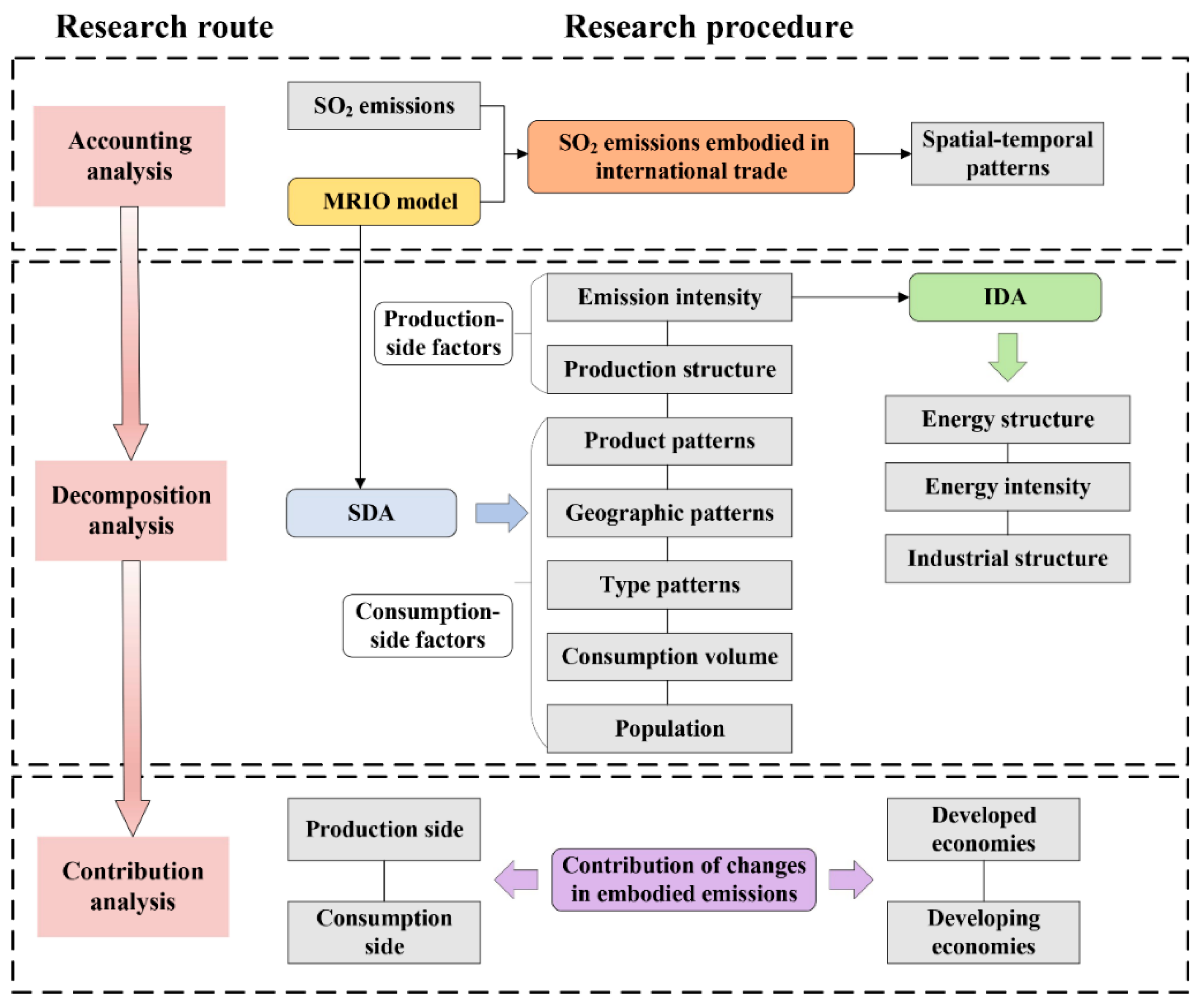
3. Materials and Methods

Following the research route of accounting–decomposition–contribution analysis, this study combined MRIO, IDA and SDA techniques to investigate the patterns and drivers of SO₂ emissions embodied in international trade and quantified the contribution of each country or region on production and consumption sides. This section will introduce the MRIO, IDA and SDA methods and show how to use them to calculate embodied SO₂ emissions and identify the driving factors. The research framework is shown in Figure 1.

3.1. Embodied Emissions in Trade

The environmentally extended multiregional input–output model was used to quantify the SO₂ emissions embodied in international trade [13]. The bilateral trade in MRIO consists of intermediate input and final use, which builds the complete production and consumption linkages between regions. Consumption-based embodied emissions are accounted based on final use, so one-unit emission may go through many regions before it eventually arrives at the final consumer.

Supposing an MRIO table with $m$ regions and $n$ sectors, the total output of sector $i$ in region $r$ ($x_i^r$) can be calculated by the following formula on the basis of the horizontal accounting balance:

$$x_i^r={\displaystyle \sum _s{\displaystyle \sum _j{z}_{ij}^{rs}}}+{\displaystyle \sum _s{y}_i^{rs}}$$

(1)

where $z_{ij}^{rs}$ denotes the intermediate input from sector $i$ in region $r$ to sector $j$ in region $s$ ($r,s=1,2,\cdots ,m$; $i,j=1,2,\cdots ,n$); $y_i^{rs}$ stands for the final use of region $s$ for commodities in sector $i$ from region $r$.

Defining $a_{ij}^{rs}=z_{ij}^{rs}/x_j^s$ as the MRIO technical coefficient [46], Equation (1) can be transferred into:

$$x_i^r={\displaystyle \sum _s{\displaystyle \sum _j{a}_{ij}^{rs}{x}_j^s}}+{\displaystyle \sum _s{y}_i^{rs}}$$

(2)

Using matrix notations, Equation (2) can be transformed into the following matrix form:

$$X=AX+{\displaystyle \sum _s{Y}^s}$$

(3)

where $A$ denotes the direct consumption matrix.

Solving for $X$ yields:

$$X={\left(I-A\right)}^{-1}\times \left({\displaystyle \sum _s{Y}^s}\right)=L\times \left({\displaystyle \sum _s{Y}^s}\right)$$

(4)

where $L={\left(I-A\right)}^{-1}$ denotes the Leontief inverse matrix, which indicates the total output required to satisfy one unit of final use.

The SO₂ extended MRIO model is constructed by adding the row vector of SO₂ emission coefficient, which describes the direct emissions per unit of total output. The total amount of embodied emissions in final demand of region $s$ can be computed by:

$$\begin{array}{ll}{F}_{Y^s}& =D^{\prime }L{Y}^s={\left[\begin{array}{l}{D}^1\\ D^2\\ ⋮\\ D^m\end{array}\right]}^T\times \left[\begin{array}{l}{L}^{11}{L}^{12}\cdots L^{1m}\\ L^{21}{L}^{22}\cdots L^{2m}\\ \cdots \cdots \cdots \cdots \\ L^{m1}{L}^{m2}\cdots L^{mm}\end{array}\right]\times \left[\begin{array}{l}{Y}^{1s}\\ Y^{2s}\\ ⋮\\ Y^{ms}\end{array}\right]\\ & ={\displaystyle \sum _r\left(D^1{}^{\prime }{L}^{1r}+D^2{}^{\prime }{L}^{2r}+\cdots +D^m{}^{\prime }{L}^{mr}\right)}\times Y^{rs}\end{array}$$

(5)

where $D^r={\left(d_i^r\right)}_{n\times 1}={\left(k_i^r/x_i^r\right)}_{n\times 1}$ denotes the column vector of SO₂ emission coefficient in region $r$; $k_i^r$ denotes the direct SO₂ emissions of sector $i$ in region $r$.

The embodied emissions in region $r$ driven by final demand in region $s$ is:

$$F_{Y^s}^r={\displaystyle \sum _t{D}^r{}^{\prime }{L}^{rt}{Y}^{ts}}$$

(6)

where $e{k}_{Y^s}^r$ denotes the flow of SO₂ emissions from region $s$ to region $r$; $L^{rt}$ is the submatrix in the Leontief inverse matrix ($t=1,2,\cdots ,m$).

3.2. Structural Decomposition Analysis

The transfer of SO₂ emissions from region $s$ to region $r$ embodied in international trade is driven by both production-side and consumption-side factors. The production technology factors at the production side and the final demand factors at the consumption side jointly affect the SO₂ flow between them. SDA based on IO model is a popular technique in measuring the contributions of different forces to changes in energy use and carbon emissions over time.

Expanding Equation (6) in matrix form yields:

$$\begin{array}{ll}{F}_{Y^s}^r& =D^r{}^{\prime }\times \left[L^{r1}{L}^{r2}\cdots L^{rm}\right]\times \left[\begin{array}{l}{Y}^{1s}\\ Y^{2s}\\ ⋮\\ Y^{ts}\\ ⋮\\ Y^{ms}\end{array}\right]\\ & =D^r{}^{\prime }\times L^r\times Y^s\left(r,s=1,2,\cdots ,m;r\ne s\right)\end{array}$$

(7)

where $L^r=\left[L^{r1}{L}^{r2}\cdots L^{rm}\right]$ denotes the input coefficient matrix of region $r$ to all the regions, which is also defined as production structure of region $r$; $Y^s$ denotes the column vector of final demand in region $s$. Equation (7) shows that the inter-regional SO₂ transfer is related to three factors (the SO₂ emission intensity, the production structure, and the consumption-side final demand). Among them, the first two factors are the driving factors in the production side, and the third factor is the driving factor in the consumption side, which together constitute the driving factors of SO₂ transfer.

To distinguish the contributions of different components in final demand, $Y$ is further decomposed into five components as follows [3]:

$$Y=\left(Y_p\circ Y_g\right)\times Y_d\times Y_v\times p$$

(8)

where the $\circ$ symbol denotes the pointwise multiplication of the corresponding elements of two matrices. $Y_d$ is a four-dimensional column vector reflecting the type patterns of the final demand. Its elements ${\alpha }_i\left(i=1,2,3,4\right)$ denote the proportion of household consumption, government investment, fixed assets formation and changes in inventories in the total final demand. $Y_p$ is a matrix composed of four column vectors corresponding to the product patterns of four kinds of final demand. Each column vector is stacked with $m$ same column vectors $\beta \left({\beta }_1={\beta }_2=\cdots ={\beta }_m\right)$, and its element is the share of the final products provided by each department. $Y_g$ is a matrix composed of four column vectors corresponding to the geographic patterns of four kinds of final demand. Each column vector is stacked with $m$ different column vectors $\eta \left({\eta }_1\ne {\eta }_2\ne \cdots \ne {\eta }_m\right)$, and its element ${\eta }_r\left(j\right)$ denotes the share of the final demand for $j$ product provided by region $r$, reflecting the regional source distribution of various final products. $Y_v$ denotes per capita consumption volume. $p$ is population. Therefore, Equation (7) can be transformed to:

$$F_{Y^s}^r=D^r{}^{\prime }\times L^r\times \left(Y_p^s\circ Y_g^s\right)\times Y_d^s\times Y_v^s\times p^s\left(r,s=1,2,\cdots ,m;r\ne s\right)$$

(9)

Equation (9) provides the computation of SO₂ transfer from region $s$ to region $r$, which is related to seven factors that include emission intensity, production structure, consumption patterns (i.e., product patterns, geographic patterns, type patterns), consumption volume and population. A total difference of Equation (9) generates Equation (10):

$$\begin{array}{l}\Delta F_{Y^s}^r=\Delta D^r{}^{\prime }\times L^r\times \left(Y_p^s\circ Y_g^s\right)\times Y_d^s\times Y_v^s\times p^s\\ +D^r{}^{\prime }\times \Delta L^r\times \left(Y_p^s\circ Y_g^s\right)\times Y_d^s\times Y_v^s\times p^s\\ +D^r{}^{\prime }\times L^r\times \left(\Delta Y_p^s\circ Y_g^s\right)\times Y_d^s\times Y_v^s\times p^s\\ +D^r{}^{\prime }\times L^r\times \left(Y_p^s\circ \Delta Y_g^s\right)\times Y_d^s\times Y_v^s\times p^s\\ +D^r{}^{\prime }\times L^r\times \left(Y_p^s\circ Y_g^s\right)\times \Delta Y_d^s\times Y_v^s\times p^s\\ +D^r{}^{\prime }\times L^r\times \left(Y_p^s\circ Y_g^s\right)\times Y_d^s\times \Delta Y_v^s\times p^s\\ +D^r{}^{\prime }\times L^r\times \left(Y_p^s\circ Y_g^s\right)\times Y_d^s\times Y_v^s\times \Delta p^s\end{array}$$

(10)

where $\Delta$ is the difference operator. Equation (10) converts seven multiplicative terms in Equation (9) into seven additive terms and fully accounts for the changes in embodied SO₂ emissions in trade. Each additive term in Equation (10) denotes the contribution of a factor assuming all other factors are constant.

Due to a unique solution for the decomposition in Equation (10) not being available [47], we followed the methods of previous studies and used the average of the so-called polar decompositions as an approximation of the average of all decompositions [48]. Solving Equation (10) with the polar decomposition method yields:

$$\begin{array}{l}\Delta F_{Y^s}^r=\frac{1}{2}\times \left[\Delta D^r{}^{\prime }{L}_{{}^0}^r\left(Y_{p,0}^s\circ Y_{g,0}^s\right)Y_{d,0}^s{Y}_{v,0}^s{p}_0^s+\Delta D^r{}^{\prime }{L}_{{}^1}^r\left(Y_{p,1}^s\circ Y_{g,1}^s\right)Y_{d,1}^s{Y}_{v,1}^s{p}_1^s\right]\\ +\frac{1}{2}\times \left[D_1^r{}^{\prime }\Delta L^r\left(Y_{p,0}^s\circ Y_{g,0}^s\right)Y_{d,0}^s{Y}_{v,0}^s{p}_0^s+D_0^r{}^{\prime }\Delta L^r\left(Y_{p,1}^s\circ Y_{g,1}^s\right)Y_{d,1}^s{Y}_{v,1}^s{p}_1^s\right]\\ +\frac{1}{2}\times \left[D_1^r{}^{\prime }{L}_1^r\left(\Delta Y_p^s\circ Y_{g,0}^s\right)Y_{d,0}^s{Y}_{v,0}^s{p}_0^s+D_0^r{}^{\prime }{L}_0^r\left(\Delta Y_p^s\circ Y_{g,1}^s\right)Y_{d,1}^s{Y}_{v,1}^s{p}_1^s\right]\\ +\frac{1}{2}\times \left[D_1^r{}^{\prime }{L}_1^r\left(Y_{p,1}^s\circ \Delta Y_g^s\right)Y_{d,0}^s{Y}_{v,0}^s{p}_0^s+D_0^r{}^{\prime }{L}_0^r\left(Y_{p,0}^s\circ \Delta Y_g^s\right)Y_{d,1}^s{Y}_{v,1}^s{p}_1^s\right]\\ +\frac{1}{2}\times \left[D_1^r{}^{\prime }{L}_1^r\left(Y_{p,1}^s\circ Y_{g,1}^s\right)\Delta Y_d^s{Y}_{v,0}^s{p}_0^s+D_0^r{}^{\prime }{L}_0^r\left(Y_{p,0}^s\circ Y_{g,0}^s\right)\Delta Y_d^s{Y}_{v,1}^s{p}_1^s\right]\\ +\frac{1}{2}\times \left[D_1^r{}^{\prime }{L}_1^r\left(Y_{p,1}^s\circ Y_{g,1}^s\right)Y_{d,1}^s\Delta Y_v^s{p}_0^s+D_0^r{}^{\prime }{L}_0^r\left(Y_{p,0}^s\circ Y_{g,0}^s\right)Y_{d,0}^s\Delta Y_v^s{p}_1^s\right]\\ +\frac{1}{2}\times \left[D_1^r{}^{\prime }{L}_1^r\left(Y_{p,1}^s\circ Y_{g,1}^s\right)Y_{d,1}^s{Y}_{v,1}^s\Delta p^s+D_0^r{}^{\prime }{L}_0^r\left(Y_{p,0}^s\circ Y_{g,0}^s\right)Y_{d,0}^s{Y}_{v,0}^s\Delta p^s\right]\\ =\Delta D+\Delta L+\Delta S_p+\Delta S_g+\Delta S_d+\Delta V+\Delta P\end{array}$$

(11)

where $\Delta F_{Y^s}^r$ denotes the changes in emission transfers between two time points; $\Delta D$, $\Delta L$, $\Delta S_p$, $\Delta S_g$, $\Delta S_d$, $\Delta V$ and $\Delta P$ denote changes in emission intensity, production structure, product patterns, geographic patterns, type patterns, consumption volume and population, respectively. The first two effects are related to the production side, while the last five effects are associated with the consumption side.

3.3. Index Decomposition Analysis

Equation (11) has decomposed changes in embodied emissions into seven factors, of which five factors are related to consumption side. By contrast, production-side factors seem not to be investigated enough, especially for emission intensity effect $\Delta D$, which could be decomposed further by using index decomposition analysis. Following the spirit of Wang et al. [43], the global SO₂ emission intensity (SEI) is typically expressed in Equation (12):

$$SEI=\frac{SE}{X}={\displaystyle \sum _{i=1}^n\frac{S{E}_i}{E_i}\frac{E_i}{X_i}}\frac{X_i}{X}$$

(12)

where $SE$ denotes global SO₂ emissions; $X$ denotes the total output; $S{E}_i$ denotes the SO₂ emissions of sector $i$; $E_i$ denotes the energy consumption of sector $i$; $X_i$ denotes the output of sector $i$.

The global SEI for time $t-1$ and $t$ can be described as Equations (13) and (14), respectively.

$$SE{I}^t={\displaystyle \sum _{i=1}^n\left(S{E}_i^t/E_i^t\right)\cdot \left(E_i^t/X_i^t\right)\cdot \left(X_i^t/X^t\right)}={\displaystyle {\sum }_{i=1}^{n}E{S}_i^t}\cdot E{I}_i^t\cdot I{S}_i^t$$

(13)

$$SE{I}^{t-1}={\displaystyle \sum _{i=1}^n\left(S{E}_i^{t-1}/E_i^{t-1}\right)\cdot \left(E_i^{t-1}/X_i^{t-1}\right)\cdot \left(X_i^{t-1}/X^{t-1}\right)}={\displaystyle {\sum }_{i=1}^{n}E{S}_i^{t-1}}\cdot E{I}_i^{t-1}\cdot I{S}_i^{t-1}$$

(14)

where $E{S}_i^t=S{E}_i^t/E_i^t$ and $E{S}_i^{t-1}=S{E}_i^{t-1}/E_i^{t-1}$, respectively, denote SO₂ emissions of unit energy consumption for sector $i$ at time $t$ and $t-1$, which could be used to represent energy structure under the assumption that the SO₂ emission factor for each kind of energy source is constant. $E{I}_i^t=E_i^t/X_i^t$ and $E{I}_i^{t-1}=E_i^{t-1}/X_i^{t-1}$, respectively, denote energy consumption of unit output (i.e., energy intensity) for sector $i$ at time $t$ and $t-1$, indicating energy efficiency level. $I{S}_i^t=X_i^t/X^t$ and $I{S}_i^{t-1}=X_i^{t-1}/X^{t-1}$, respectively, denote the share of output of sector $i$ at time $t$ and $t-1$, which could be used to represent industrial structure.

Suppose that the global SEI varies from time $t-1$ to $t$ (i.e., $V_{tot}^{t-1,t}=SE{I}^t-SE{I}^{t-1}$). Such a change can be expressed in the following additive form [49] as Equation (15), which indicates that global SEI change is related to three factors: energy structure, energy intensity and industrial structure.

$$\begin{array}{l}{V}_{tot}^{t-1,t}=SE{I}^t-SE{I}^{t-1}=V_{ES}^{t-1,t}+V_{EI}^{t-1,t}+V_{IS}^{t-1,t}\\ V_{ES}^{t-1,t}={\displaystyle \sum _{i=1}^n{\omega }_i\ln }\frac{E{S}_i^t}{E{S}_i^{t-1}}\\ V_{EI}^{t-1,t}={\displaystyle \sum _{i=1}^n{\omega }_i\ln }\frac{E{I}_i^t}{E{I}_i^{t-1}}\\ V_{IS}^{t-1,t}={\displaystyle \sum _{i=1}^n{\omega }_i\ln \frac{I{S}_i^t}{I{S}_i^{t-1}}}\\ {\omega }_i=L\left(SE{I}_i^{t-1},SE{I}_i^t\right)=\frac{SE{I}_i^{t-1}-SE{I}_i^t}{\ln SE{I}_i^{t-1}-\ln SE{I}_i^t}\end{array}$$

(15)

where $V_{ES}^{t-1,t}$, $V_{EI}^{t-1,t}$ and $V_{IS}^{t-1,t}$, respectively, measure the effects of energy structure, energy intensity and industrial structure over the period $\left[t-1,t\right]$; ${\omega }_i$ denotes the weight of sector $i$, and $L\left(a,b\right)=\left(b-a\right)/\left(\ln b-\ln a\right)$ is the logarithmic mean function.

Equation (15) describes the single-period decomposition results of SEI change. In the case of multi-period decomposition, the accumulative effect $V_{tot}^{0,T}$ from time $0$ to $T$ can be calculated by Equation (16):

$$\begin{array}{ll}{V}_{tot}^{0,T}& =SE{I}^T-SE{I}^0={\displaystyle \sum _{t=1}^T\left(SE{I}^t-SE{I}^{t-1}\right)}\\ & ={\displaystyle \sum _{t=1}^T\left(V_{ES}^{t-1,t}+V_{EI}^{t-1,t}+V_{IS}^{t-1,t}\right)}\\ & =V_{ES}^{0,T}+V_{EI}^{0,T}+V_{IS}^{0,T}\end{array}$$

(16)

where $V_{ES}^{0,T}$, $V_{EI}^{0,T}$ and $V_{IS}^{0,T}$ are the corresponding cumulative sum of single-period decomposed indexes.

3.4. Data Sources

Data used in this study include monetary MRIO tables and SO₂ emissions data of countries or regions. The related data were gathered from the Eora global supply chain database [50], which provides a time series of high-resolution IO tables with matching environmental and social satellite accounts for 189 countries or regions (https://worldmrio.com/ (accessed on 12 May 2018)). Eora has been applied in some excellent works, such as Peters et al. [51], Yang et al. [52] and Lin et al. [53], so the data credibility can be guaranteed. In order to eliminate the impact of price change, MRIO tables in 1996 to 2015 were deflated to 1995 constant price.

4. Results

This section will present the accounting, decomposition and contribution results to reveal the patterns and drivers of change in the embodied SO₂ emissions and compare the contributions of different economies on the production and consumption sides.

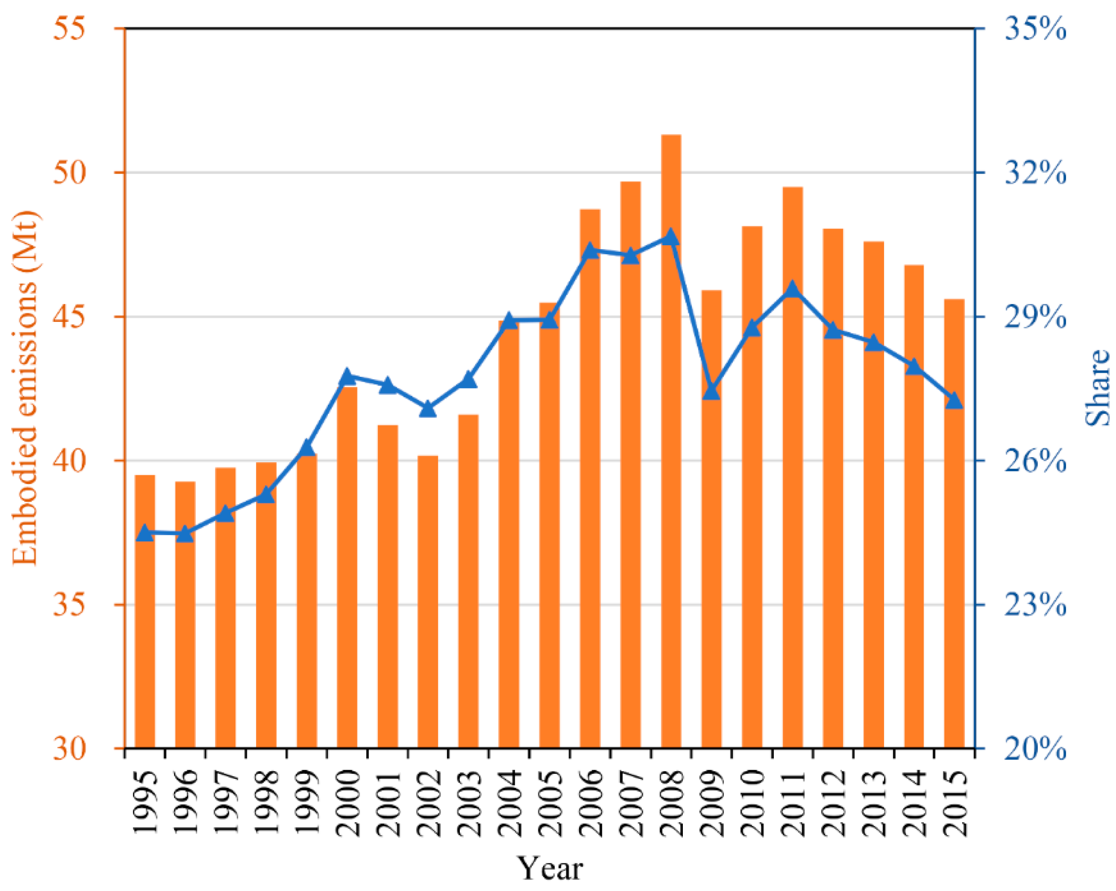
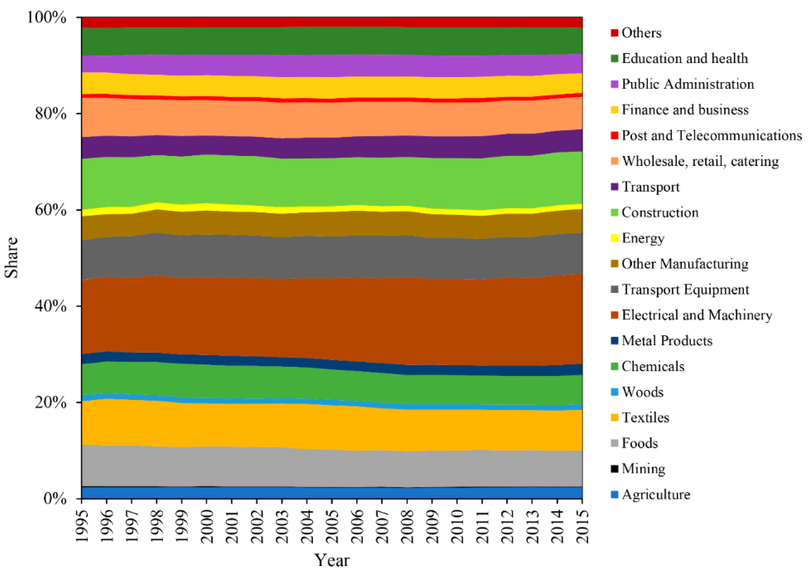
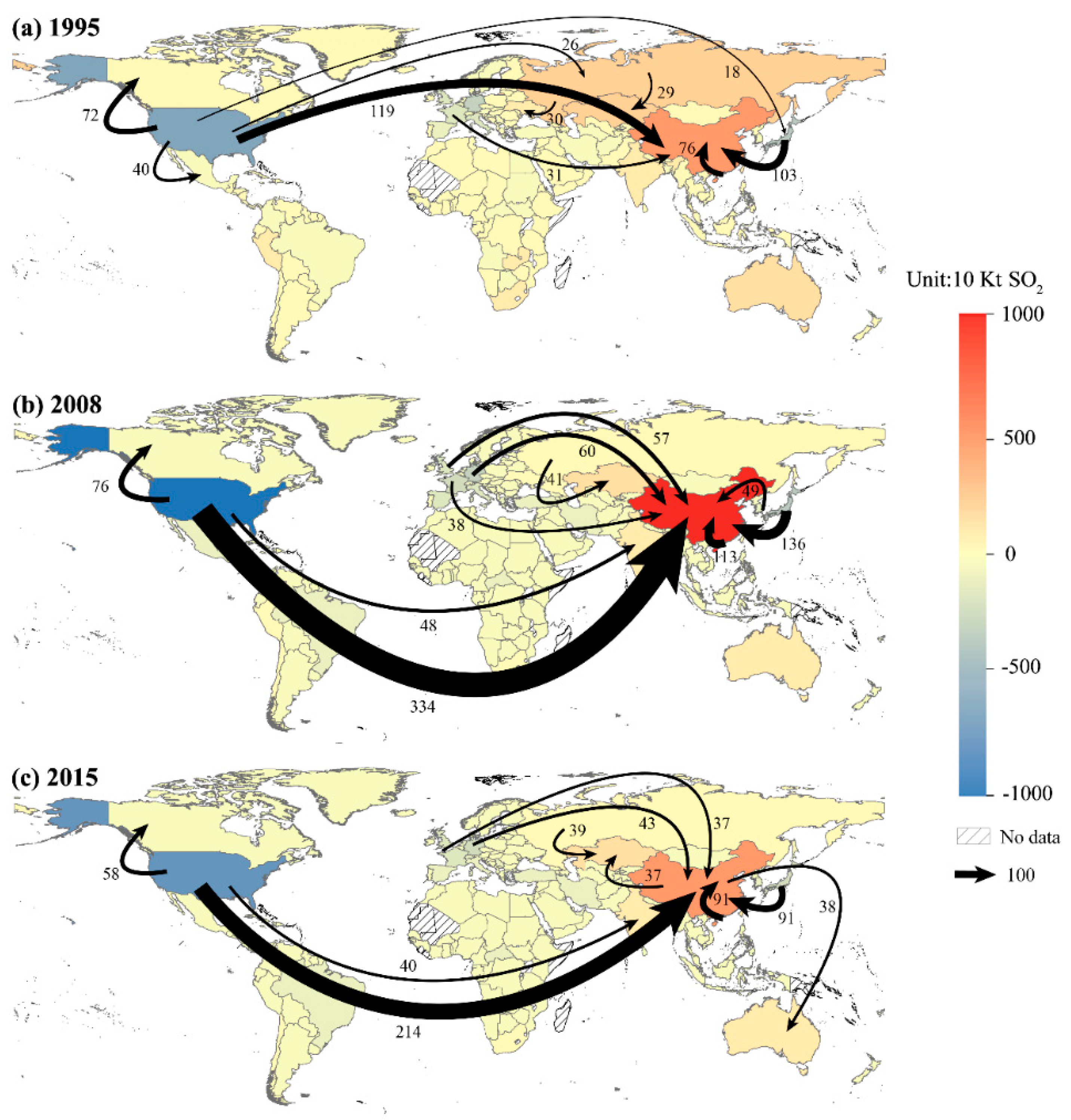
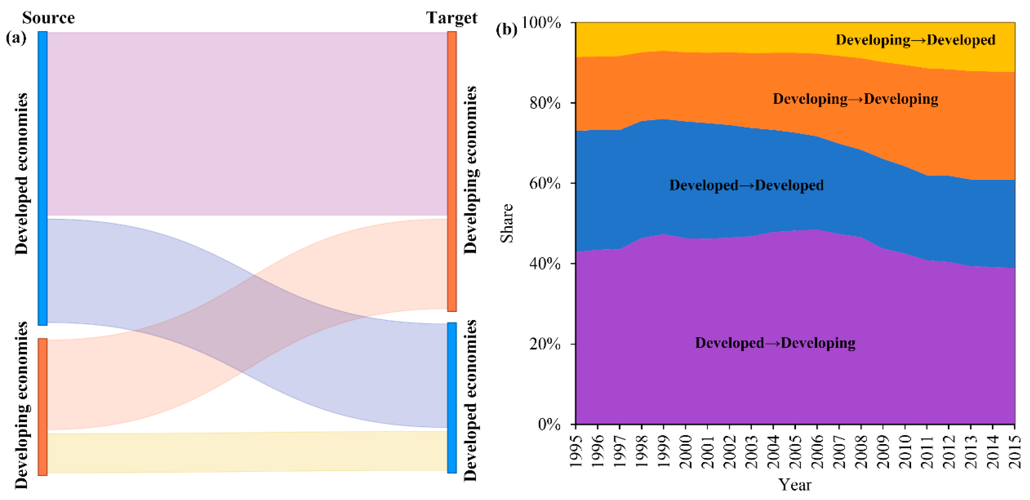
4.1. Patterns of Emissions Embodied in International Trade

The SO₂ emissions embodied in international trade accounted for about 24–30% of the global emissions from 1995 to 2015 (Figure 2, blue line). Meanwhile, the absolute embodied emissions ranged from a low of 39.3 Mt in 1996 to a high of 51.3 Mt in 2008 (Figure 2, orange bar), presenting significant temporal variation characteristics that trended upward between 1995 and 2008 but downward between 2008 and 2015. The finding that the SO₂ emissions embodied in international trade decreased after 2008 has been revealed in existing literature [32]. Nevertheless, our analysis of more recent data, up to 2015, permits the more confident conclusion that the global embodied emissions peaked in 2008.

Specifically, in the period from 1995 to 2002, global embodied SO₂ emissions underwent a slight increase from 39.5 Mt to 40.2 Mt in a fluctuating way. Notably, the embodied emissions reached a relatively high point in 2000, but then declined in 2001 and 2002 (Figure 2, orange bar). In fact, due to the worldwide economic recession caused by the dotcom bubble burst in 2001, global trade slowed down in 2001 and 2002 [54], thereby resulting in the decline in embodied emissions.

In the period from 2002 until 2008, when the global financial crisis occurred, embodied SO₂ emissions in international trade grew fast (Figure 2, orange bar). This tendency has also been revealed by other studies regarding carbon emissions [22,55], pollutant emissions [3] and metal use [56]. As shown in Figure 2, embodied emissions increased by 11.1 Mt from 2002 to 2008, which accounted for 58.6% of global total SO₂ emissions growth in the same period. Actually, China’s accession into the WTO stimulated the rapid growth of global trade and exacerbated the geospatial separation between the regions consuming commodities and regions where products and related SO₂ pollution are produced, thereby resulting in the dramatic growth in embodied emissions. From a sectoral point of view, a large share of embodied SO₂ emissions growth in this period was attributed to the machinery and equipment manufacturing industry (Figure 3, grey and dark orange shading). For instance, emissions embodied in the final use of electrical and machinery products grew significantly, contributing 2.8 Mt SO₂ to the global embodied emissions between 2002 and 2008, which accounted for 25.2% of the total embodied emissions growth over the same period (Figure 3, dark orange shading).

The embodied SO₂ emissions underwent a downward trend between 2008 and 2015 and decreased from 51.3 Mt to 45.6 Mt, a total decline of 11.1% (Figure 2, orange bar). In the immediate aftermath of the global financial crisis, the sharp drop in the final consumption for goods and services abroad was primarily responsible for the decline between 2008 and 2009. The international trade volume decreased by about 12% in this period, bringing about a 10.5% decline in embodied emissions. Then, embodied emissions grew by 7.8% from 2009 to 2011, which may be attributed to the recovery of the global economy and trade. Emissions were also founded to decrease by an average of 1.6% per year between 2011 and 2015, although the global economy had emerged from the recession (Figure 2, orange bar).

Spatially, Figure 4, plotted by ArcGIS 10.2.2, maps the inter-regional SO₂ transfers via international trade and resulting SO₂ trade balance (i.e., the difference between SO₂ inflows and outflows) in different regions. The shading of regions in Figure 4 denotes the magnitude of net inflows (red) or net outflows (blue) embodied in international trade in 1995, 2008 and 2015. Arrows in the figure denote the ten largest inter-regional SO₂ flows. The number and arrow thickness indicate emissions embodied in flows.

From the perspective of SO₂ trade balance, the largest net SO₂ exporters primarily were developed economies, such as the USA, Japan, Germany, UK, France and Chinese Hong Kong, while developing economies (e.g., Chinese mainland, Kazakhstan, India, Russia) and resource-abundant economies (e.g., Australia) were the highest net SO₂ importers. Especially, the USA and Chinese mainland served as the largest source and sink of global SO₂ transfers, respectively. The net SO₂ inflows of the USA in 1995, 2008 and 2015 were –4.5, –9.3 and –6.6 Mt, respectively, while those of the Chinese mainland were 4.8, 9.8 and 4.9 Mt, respectively.

Looking at the inter-regional SO₂ flows, the largest one was the flow from the USA to Chinese mainland, which transferred emissions of 1190.4, 3342.0 and 2137.1 Kt in 1995, 2008 and 2015, respectively. Clearly, it also increased firstly and then decreased, corresponding to the inversed “U” trend of the total embodied emissions. The following notable flows included Japan→Chinese mainland, USA→Canada, Chinese Hong Kong→ Chinese mainland. Generally, the global embodied SO₂ emissions were mainly transferred from west to east and from developing to developed economies (Figure 4).

Figure 5a indicates the accumulative SO₂ flows between developed and developing economies from 1995 to 2015. It is found that developed economies transferred 415.2 Mt SO₂ to developing economies via international trade between 1995 and 2015, accounting for 44.4% of the total embodied SO₂ emissions (Figure 5a, purple belt). In contrast, developing economies only transferred about one-in-five (85.4 Mt) back to developed economies (Figure 5a, yellow belt). As a result, the pollution emissions grew rapidly in some developing economies but stabilized or even decreased in many developed economies in recent years. Actually, due to the pollution intensive energy mix, less efficient production technologies as well as an inferior position in the global value chain, developing economies contributed a large amount of energy- and emission-intensive final and intermediate products to support the production and consumption of finished goods in developed economies [57]. Additionally, notable variations in the flow patterns between developed and developing economies were observed over this period. As shown in Figure 5b, the share of developed → developing economies decreased to 38.9%, while that of developing → developed economies increased to 12.3%. Notably, the share of developing → developing economies witnessed considerable growth from 18.3% in 1995 to 26.8% in 2015 (Figure 5b, orange shading), which may be attributed to the rapid rise of south–south trade since the global financial crisis [48].

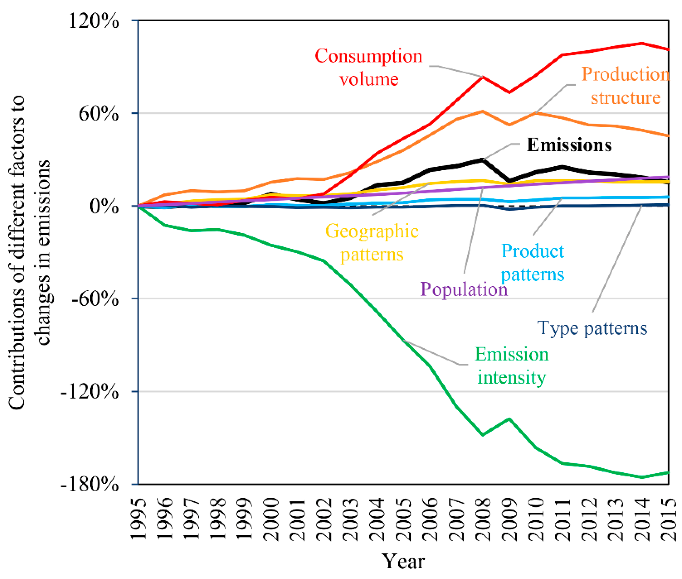
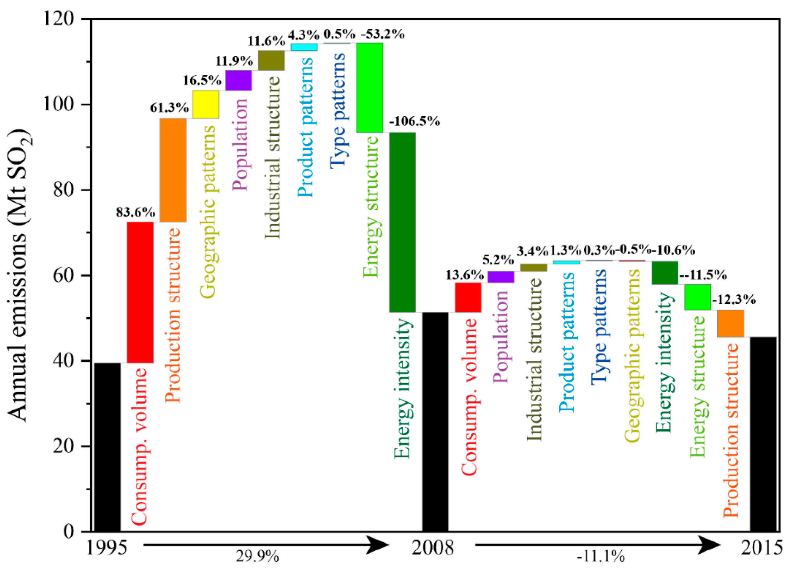
4.2. Determinants of Changes in Emissions Embodied in International Trade

Equation (11) was used to decompose the changes in embodied emissions from 1995 to 2015. As shown in Figure 6, global embodied SO₂ emissions increased by 15.4% in this period (Figure 6, black curve). The increase was dominated by the expansion in consumption volume, which—in the absence of other factors—would have caused embodied emissions to increase by 101.2% over the two decades (Figure 6, red curve). The next most important driver during this time frame was production structure, which contributed to a 45.3% increase during this period (Figure 6, orange curve). The effects of population and geographic patterns of final consumption played a similar upward influence on emissions, corresponding to the contributions of 18.7% (Figure 6, purple curve) and 15.9% (Figure 6, yellow curve), respectively. The product and type patterns of final consumption had minor impacts on emissions (Figure 6, blue and dark blue curves). On the other hand, emission intensity was the only factor to decrease emissions between 1995 and 2015 (Figure 6, green curve), the decline in which resulted in notable reductions in embodied emissions. If other factors were kept constant, it would have caused embodied emissions to decrease by 172.5% over this period (Figure 6, green curve). Notably, the decline in emissions between 2011 and 2015 is not owing to the crisis because the consumption volume still made an upward influence on emissions in this period (Figure 6, red curve) but was dominated by energy and production system transitions (Figure 6, orange and green curves).

In order to reveal more production-related factors, Equation (15) was used to decompose the changes in SO₂ emission intensity from 1995 to 2015. As shown in Figure 7, global emission intensity decreased by 62.7% in this period (Figure 7, black curve). Our analysis shows that the main factor behind this decrease was the decrease in energy intensity, which corresponds to a contribution of a 43.7% decrease in emission intensity over this period (Figure 7, green curve). The next most important factor was energy structure, which contributed a 24.8% decrease in emission intensity (Figure 7, cyan curve). However, the effect of industrial structure exerted an upward influence of 5.8% (Figure 7, dark yellow curve).

In light of the global embodied emissions peaking in 2008, we divided the whole period into two subperiods, 1995–2008 and 2008–2015, so as to investigate the drivers behind the peaking emissions.

Growing emissions from 1995 to 2008. In the period from 1995 to 2008, the global embodied SO₂ emissions increased by 29.9% (Figure 8, black bar). The increase was dominated by the expansion in consumption volume (83.6%; Figure 8, red bar), followed by production structure (61.3%, Figure 8, red bar). The effects of consumption patterns-related factors, such as geographic patterns, product patterns and type patterns, contributed 16.5%, 4.3% and 0.5% increases to emissions, respectively (Figure 8, yellow, blue and dark blue bars). Other promoting factors, such as population and industrial structure, exerted modest upward influences of 11.9% and 11.6% on emissions, respectively (Figure 8, purple and dark yellow bars). However, the upward influence of the above seven factors was largely offset by the downward influence of energy intensity and energy structure, which contributed 106.5% and 53.2% decreases to emissions, respectively (Figure 8, green and cyan bars).

Declining emissions from 2008 to 2015. The global embodied emissions stopped increasing in 2008 and declined by 11.1% from 2008 to 2015 (Figure 8, black bar). During this time period, the effects of consumption volume, population, industrial structure, product patterns and type patterns still acted as the drivers increasing embodied emissions by 13.6%, 5.2%, 3.4%, 1.3% and 0.3%, respectively (Figure 8, red, purple, dark yellow, blue and dark blue bars). While the consumption volume still caused an upward influence on emissions, the magnitude underwent a sharp decline from 83.6% to 13.6%. As a result, the upward influence of the five factors was overwhelmed by the downward influence of production structure (–12.3%), energy structure (–11.5%), energy intensity (–10.6%) and geographic patterns (–0.5%; Figure 8, orange, cyan, green and yellow bars). Notably, shifts in production structure switched from a significant promoting factor between 1995 and 2008 (61.3%) to the dominant inhabiting factor between 2008 and 2015 (–12.3%; Figure 8, orange bars). This may be because the volume and type of intermediate products consumed by various industry sectors at home and abroad has evolved and become more efficient [39]. Taken together, production-side effects, such as energy and production system transitions and the slowdown in international trade, were primarily responsible for the peak in embodied emissions in international trade.

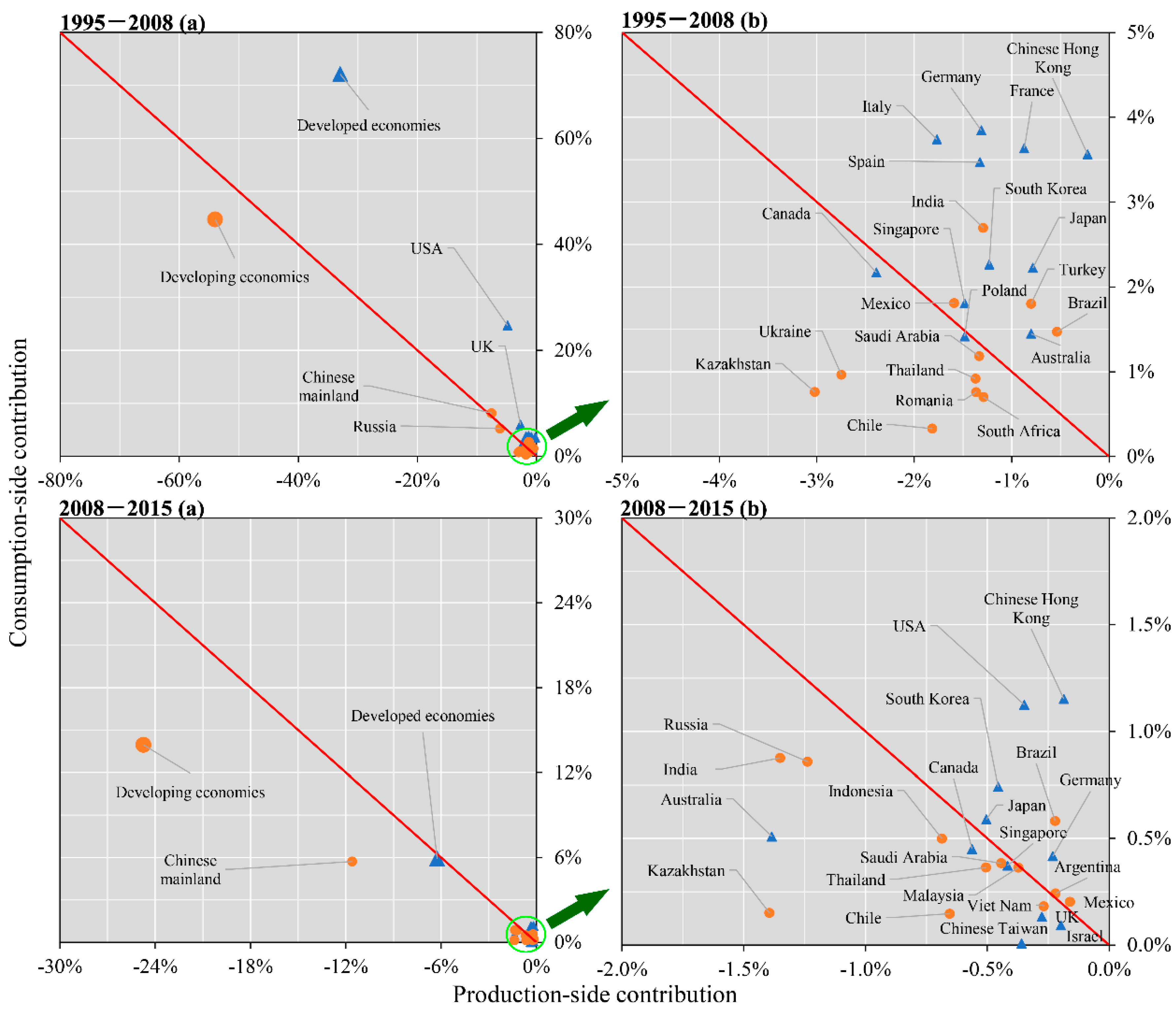
4.3. Production- and Consumption-Side Contributions of Regions

We further calculated the contribution of each region to the changes in global embodied emissions for the periods 1995–2008 and 2008–2015 on the production and consumption sides. As shown in Figure 9, the horizontal and vertical axes denote the contribution rates on production and consumption sides, respectively. The red line in the figure is a straight line with a slope of −1 passing through the origin. Figure 9a,b are the contribution results for period 1995–2008, and Figure 9b is the enlarged version of the inner part of the green ellipse in Figure 9a so as to present the distribution of each point more clearly. Similarly, Figure 9a,b correspond to the period 2008–2015. Blue triangle points and orange round points stand for developed and developing economies, respectively. Due to the limited space, only 30 major economies with the largest contributions were presented in Figure 9.

As can be seen from Figure 9, all points fell in the second quadrant, indicating that all the 30 main economies, in both periods 1995–2008 and 2008–2015, contributed negatively to the change in embodied emissions on the production side, while they made a positive contribution to emissions on the consumption side. However, the relative size of production- and consumption-side contributions varied greatly in different regions, resulting in significant differences in the total contribution of regions. The point below the red line indicates that the total contribution of the region was negative; that is, the upward influence on the consumption side was offset by the downward influence on the production side and vice versa. In general, developed economies are mainly located above the red line (Figure 9, blue triangle points), while developing economies are below the red line (Figure 9, orange round points).

In the period 1995–2008, as shown in Figure 9a,b, Kazakhstan had the largest negative contribution (−2.3%), which was attributable to its great efforts toward a clean energy structure through the use of policy and technology [58], thereby causing a significant downward influence on the production side (−3.0%). On the contrary, the USA was found to have the largest positive contribution (19.8%), which was mainly due to its huge upward influence on the consumption side (24.7%). Notably, the Chinese mainland had the second largest production-side contribution (8.2%) resulting from its huge population base and corresponding final demand growth [59]. However, the significant upward influence was largely offset by its huge downward influence on the production side (−7.6%), thereby exerting a minor upward influence on global emissions.

In the period 2008–2015, as shown in Figure 9a,b, the Chinese mainland became the largest contributor to reduce global embodied SO₂ emissions (−5.9%). This may be attributed to its recent great efforts in energy-saving and emission reduction [60], which largely removed SO₂ emissions from the production process, thereby amounting to the remarkable negative contribution on the production side (−11.6%). Notably, the consumption-side positive contribution of the USA also met a sharp decline from 24.7% between 1995 and 2008 to 1.1% between 2008 and 2015. A similar condition was also observed for the UK, Germany and Chinese Hong Kong. As a result, some developed economies, such as the UK, Australia, Canada and Singapore, fell below the red line and the whole developed economies switched to exert a downward influence on global emissions. This is because developed economies became less dependent on imports after the financial crisis, hence slowing down the emissions embodied in international trade on the consumption side [61].

5. Discussion

The SO₂ emissions embodied in international trade experienced an inverted U-shape changing trend. They grew dramatically before the global financial crisis, which was mainly attributable to the expansion in the consumption volume and shifts in the production structure, while the dramatic shift after 2008 was mainly due to production-side factors (i.e., shifts in production structure, decline in energy intensity and shifts in energy structure).

Developing economies, such as the Chinese mainland and Kazakhstan, contributed a significant decrease to global emissions. This may be attributed to their great efforts toward clean energy structures through the use of policy and technology [58]. Additionally, the Chinese government has made great efforts to reduce the SO₂ emissions from the production side through implementing a mandatory emissions control system [62,63,64]. With the implementation of measures that include shutting down small thermal power units and installing desulfurization facilities, considerable emissions have been removed since 2008 [1]. Meanwhile, the volume and type of intermediate products consumed by various industry sectors at home and abroad has evolved and become more efficient [39], thereby bringing about the significant downward influence of the production structure between 2008 and 2015. The deglobalization has resulted in a significant decrease in the upward influence of the consumption volume on emissions between 1995 and 2008 and 2008 and 2015, which is also an important reason for the peak and decline in emissions.

The transfers of SO₂ emissions tended to flow from developed economies, such as the USA, to less developed ones, such as the Chinese mainland. Actually, developed countries imported high energy- and emission-intensive products from developing countries to meet their final demands instead of producing them by themselves, thereby resulting in large SO₂ transfers from developed to developing economies. However, there has been some decrease in the amount after the financial crisis because developed economies became less dependent on imports [61]. Moreover, the decline in their final demands for products abroad reduced their upward influence on the consumption side, and some, such as the UK, Australia, Canada and Singapore, even switched to contribute a decrease in the global emissions. On the contrary, the SO₂ flowing between developing economies witnessed a significant increase, which may be attributed to the rapid rise of south–south trade since the global financial crisis [48].

6. Conclusions and Policy Implications

6.1. Conclusions

This study investigated the patterns and drivers of the trends in the SO₂ emissions embodied in international trade from 1995 to 2015. Some interesting findings have been revealed:

First, the SO₂ emissions embodied in international trade accounted for about 24%–30% of the global emissions between 1995 and 2015. The global embodied emissions increased at an accelerated rate before the global financial crisis and peaked at 51.3 Mt in 2008, followed by a fluctuating decline from 2008 to 2015. Spatially, the transfers of SO₂ emissions tended to flow from developed countries to developing countries, but the trend has weakened after the financial crisis.

Second, the increase before 2008 was dominated by the expansion in the consumption volume, especially for the products of the machinery and equipment manufacturing industry, but its upward influence significantly decreased between 2008 and 2015 due to deglobalization. Even more, shifts in the production structure switched from a significant promoting factor between 1995 and 2008 to the dominant inhabiting factor between 2008 and 2015.

Third, more developing economies, including the Chinese mainland, contributed negatively to the global embodied emissions growth, while more developed economies, such as the USA, were found to contribute an increase to emissions, but the upward influence has decreased significantly after the crisis.

Fourth, the negative contribution of developing economies on the production side offsets their positive contribution on the consumption side, while developed economies are just the opposite. Nevertheless, the consumption-side contribution of developed economies has decreased after the crisis, thereby resulting in the weakening upward influence on emissions. Taken together, energy and production technology upgrading and energy structure and declining final demands for products abroad in developed countries both accounted for the peak and decline in the global embodied SO₂ emissions.

6.2. Policy Implications

According to the above findings, several policy implications can be summarized as follows.

Since the SO₂ emissions embodied in international trade accounted for about a quarter of the global emissions, the adverse impact of international trade on the world’s eco-environment cannot be ignored. Meanwhile, in the context of large amounts of SO₂ emissions transferred from developed regions to developing regions, the allocation of pollutant emission reduction responsibilities based on production-based accounting is obviously lacking justice for developing countries. Therefore, the pollution mitigation tasks should be reasonably distributed among the countries to reduce SO₂ leakage in international trade, and attention should be paid to the impact of international trade to prevent developed countries from outsourcing more pollution to others. Developed and developing countries need to be treated differently when it comes to formulating a global pollutant emission reduction policy. Developed countries such as the USA have removed the production of resources abroad or imported substitutes to circumvent their own emission reduction responsibilities. To this end, the international community should urge developed countries to take on more reduction responsibilities and push technology transfer or offer financial aid to improve other countries’ technology for dealing with pollutants.

Since developing countries’ production-side factors, such as energy and production system transitions, significantly contributed to decreasing emissions, policymakers in developing countries should continue to maintain their current policies on energy production, industrial technology and environmental regulation. Additionally, environmental subsidies would help fund firms to upgrade their desulfurization technologies, eliminate outdated production technologies and apply clean energy resources. Greater international cooperation and support are strongly recommended to promote technology transfer, and effective supervision should also occur regarding the implementation and operation of these imported technologies. On the other hand, as developed countries’ consumption-side factors, such as consumption volume and patterns, contributed to increasing the embodied emissions throughout the whole period, developed countries should correctly guide the consumption concept of residents to help curb luxury consumption and promote green consumption habits.

References

1. Xing, Z.; Wang, J.; Feng, K.; Hubacek, K. Decline of net SO2 emission intensity in China’s thermal power generation: Decomposition and attribution analysis. Sci. Total Environ. 2020, 719, 137367. [Google Scholar] [CrossRef]
2. Xu, C.; Zhao, W.; Zhang, M.; Cheng, B. Pollution haven or halo? The role of the energy transition in the impact of FDI on SO2 emissions. Sci. Total Environ. 2020, 763, 143002. [Google Scholar] [CrossRef] [PubMed]
3. Meng, J.; Yang, H.; Yi, K.; Liu, J.; Guan, D.; Liu, Z.; Mi, Z.; Coffman, D.M.; Wang, X.; Zhong, Q.; et al. The slowdown in global air-pollutant emission growth and driving factors. One Earth 2019, 1, 138–148. [Google Scholar] [CrossRef] [Green Version]
4. Li, Y.L.; Chen, B.; Chen, G.Q. Carbon network embodied in international trade: Global structural evolution and its policy implications. Energy Policy 2020, 139, 111316. [Google Scholar] [CrossRef]
5. Chen, W.; Qu, S.; Han, M.S. Environmental implications of changes in China’s inter-provincial trade structure. Resour. Conserv. Recycl. 2021, 167, 105419. [Google Scholar] [CrossRef]
6. Cherniwchan, J.; Copeland, B.R.; Taylor, M.S. Trade and the environment: New methods, measurements, and results. Annu. Rev. Econ. 2017, 9, 59–85. [Google Scholar] [CrossRef] [Green Version]
7. Mao, X.; He, C. A trade-related pollution trap for economies in transition? Evidence from China. J. Clean. Prod. 2018, 200, 781–790. [Google Scholar] [CrossRef]
8. Wang, S.; He, Y.; Song, M. Global value chains, technological progress, and environmental pollution: Inequality towards developing countries. J. Environ. Manag. 2021, 277, 110999. [Google Scholar] [CrossRef]
9. Liang, S.; Stylianou, K.S.; Jolliet, O.; Supekar, S.; Qu, S.; Skerlos, S.J.; Xu, M. Consumption-based human health impacts of primary PM2. 5: The hidden burden of international trade. J. Clean. Prod. 2017, 167, 133–139. [Google Scholar] [CrossRef]
10. Greenaway, D.; Hine, R.; Milner, C. Vertical and horizontal intra-industry trade: A cross industry analysis for the United Kingdom. Econ. J. 1995, 105, 1505–1518. [Google Scholar] [CrossRef]
11. Leitão, N.C.; Balogh, J.M. The impact of intra-industry trade on carbon dioxide emissions: The case of the European Union. Agric. Econ. 2020, 66, 203–214. [Google Scholar] [CrossRef]
12. Leitão, N.C. Testing the role of trade on carbon dioxide emissions in Portugal. Economies 2021, 9, 22. [Google Scholar] [CrossRef]
13. Leontief, W. Environmental repercussions and the economic structure: An input-output approach. Rev. Econ. Statis. 1970, 52, 262–271. [Google Scholar] [CrossRef]
14. Wiedmann, T.; Lenzen, M. Environmental and social footprints of international trade. Nat. Geosci. 2018, 11, 314–321. [Google Scholar] [CrossRef]
15. Jiang, L.; He, S.; Tian, X.; Zhang, B.; Zhou, H. Energy use embodied in international trade of 39 countries: Spatial transfer patterns and driving factors. Energy 2020, 195, 116988. [Google Scholar] [CrossRef]
16. Wang, W.; Hu, Y. The measurement and influencing factors of carbon transfers embodied in inter-provincial trade in China. J. Clean. Prod. 2020, 270, 122460. [Google Scholar] [CrossRef]
17. Chen, X.; Liu, W.; Zhang, J.; Li, Z. The change pattern and driving factors of embodied SO2 emissions in China’s inter-provincial trade. J. Clean. Prod. 2020, 276, 123324. [Google Scholar] [CrossRef]
18. Li, Q.; Wu, S.; Lei, Y.; Li, S.; Li, L. Evolutionary path and driving forces of inter-industry transfer of CO2 emissions in China: Evidence from structural path and decomposition analysis. Sci. Total Environ. 2020, 765, 142773. [Google Scholar] [CrossRef]
19. Zhen, W.; Li, J. The formation and transmission of upstream and downstream sectoral carbon emission responsibilities: Evidence from China. Sustain. Prod. Consump. 2021, 25, 563–576. [Google Scholar] [CrossRef]
20. Feng, K.; Davis, S.J.; Sun, L.; Li, X.; Guan, D.; Liu, W.; Liu, Z.; Hubacek, K. Outsourcing CO2 within china. Proc. Natl. Acad. Sci. USA 2013, 110, 11654–11659. [Google Scholar] [CrossRef] [Green Version]
21. Zheng, H.; Xu, L. Production and consumption-based primary PM2.5 emissions: Empirical analysis from China’s interprovincial trade. Resour. Conserv. Recycl. 2020, 155, 104661. [Google Scholar] [CrossRef]
22. Zhang, Z.; Guan, D.; Wang, R.; Meng, J.; Zheng, H.; Zhu, K.; Du, H. Embodied carbon emissions in the supply chains of multinational enterprises. Nat. Clim. Chang. 2020, 10, 1096–1101. [Google Scholar] [CrossRef]
23. Wu, X.; Li, C.; Guo, J.; Wu, X.; Meng, J.; Chen, G. Extended carbon footprint and emission transfer of world regions: With both primary and intermediate inputs into account. Sci. Total Environ. 2021, 775, 145578. [Google Scholar] [CrossRef]
24. Arce, G.; López, L.A.; Guan, D. Carbon emissions embodied in international trade: The post-China era. Appl. Energy 2016, 184, 1063–1072. [Google Scholar] [CrossRef]
25. Oita, A.; Malik, A.; Kanemoto, K.; Geschke, A.; Nishijima, S.; Lenzen, M. Substantial nitrogen pollution embedded in international trade. Nat. Geosci. 2016, 9, 111–115. [Google Scholar] [CrossRef]
26. Liu, Q.; Long, Y.; Wang, C.; Wang, Z.; Wang, Q.; Guan, D. Drivers of provincial SO2 emissions in China–Based on multi-regional input-output analysis. J. Clean. Prod. 2019, 238, 117893. [Google Scholar] [CrossRef]
27. Wang, Z.; Li, C.; Liu, Q.; Niu, B.; Peng, S.; Deng, L.; Kang, P.; Zhang, X. Pollution haven hypothesis of domestic trade in China: A perspective of SO2 emissions. Sci. Total Environ. 2019, 663, 198–205. [Google Scholar] [CrossRef]
28. Yang, X.; Zhang, W.; Fan, J.; Li, J.; Meng, J. The temporal variation of SO2 emissions embodied in Chinese supply chains, 2002–2012. Environ. Pollut. 2018, 241, 172–181. [Google Scholar] [CrossRef]
29. Liu, Z.; Song, P.; Mao, X. Accounting the effects of WTO accession on trade-embodied emissions: Evidence from China. J. Clean. Prod. 2016, 139, 1383–1390. [Google Scholar] [CrossRef]
30. Chuai, X.; Lu, Q.; Li, J. Footprint of SO2 in China’s international trade and the interregional hotspot analysis. Appl. Geogr. 2020, 125, 102282. [Google Scholar] [CrossRef]
31. Islam, M.; Kanemoto, K.; Managi, S. Impact of trade openness and sector trade on embodied greenhouse gases emissions and air pollutants. J. Ind. Ecol. 2016, 20, 494–505. [Google Scholar] [CrossRef] [Green Version]
32. Zhong, Z.; Zhang, X.; Bao, Z. Spatial characteristics and driving factors of global energy-related sulfur oxides emissions transferring via international trade. J. Environ. Manag. 2019, 249, 109370. [Google Scholar] [CrossRef] [PubMed]
33. Ang, B.W. Decomposition analysis for policymaking in energy: Which is the preferred method? Energy Policy 2004, 32, 1131–1139. [Google Scholar] [CrossRef]
34. Su, B.; Ang, B.W.; Li, Y. Structural path and decomposition analysis of aggregate embodied energy and emission intensities. Energy Econ. 2019, 83, 345–360. [Google Scholar] [CrossRef]
35. Li, D.; Huang, G.; Zhang, G.; Wang, J. Driving factors of total carbon emissions from the construction industry in Jiangsu Province, China. J. Clean. Prod. 2020, 276, 123179. [Google Scholar] [CrossRef]
36. Li, W.; Xu, D.; Li, G.; Su, B. Structural path and decomposition analysis of aggregate embodied energy intensities in China, 2012–2017. J. Clean. Prod. 2020, 276, 124185. [Google Scholar] [CrossRef]
37. Wang, X.; Huang, H.; Hong, J.; Ni, D.; He, R. A spatiotemporal investigation of energy-driven factors in China: A region-based structural decomposition analysis. Energy 2020, 207, 118249. [Google Scholar] [CrossRef]
38. Kim, T.J.; Tromp, N. Carbon emissions embodied in China-Brazil trade: Trends and driving factors. J. Clean. Prod. 2021, 293, 126206. [Google Scholar] [CrossRef]
39. Feng, K.; Davis, S.J.; Sun, L.; Hubacek, K. Drivers of the US CO2 emissions 1997–2013. Nat. Commun. 2015, 6, 1–8. [Google Scholar] [CrossRef] [Green Version]
40. Zheng, J.; Mi, Z.; Coffman, D.M.; Shan, Y.; Guan, D.; Wang, S. The slowdown in China’s carbon emissions growth in the new phase of economic development. One Earth 2019, 1, 240–253. [Google Scholar] [CrossRef] [Green Version]
41. Yuan, X.; Teng, Y.; Yuan, Q.; Liu, M.; Fan, X.; Wang, Q.; Ma, Q.; Hong, J.; Zuo, J. Economic transition and industrial sulfur dioxide emissions in the Chinese economy. Sci. Total Environ. 2020, 744, 140826. [Google Scholar] [CrossRef] [PubMed]
42. Yang, X.; Wang, S.; Zhang, W.; Li, J.; Zou, Y. Impacts of energy consumption, energy structure, and treatment technology on SO2 emissions: A multi-scale LMDI decomposition analysis in China. Appl. Energy 2016, 184, 714–726. [Google Scholar] [CrossRef]
43. Wang, Q.; Wang, Y.; Zhou, P.; Wei, H. Whole process decomposition of energy-related SO2 in Jiangsu Province, China. Appl. Energy 2017, 194, 679–687. [Google Scholar] [CrossRef]
44. Hang, Y.; Wang, Q.; Wang, Y.; Su, B.; Zhou, D. Industrial SO2 emissions treatment in China: A temporal-spatial whole process decomposition analysis. J. Environ. Manag. 2019, 243, 419–434. [Google Scholar] [CrossRef]
45. Zhang, P. End-of-pipe or process-integrated: Evidence from LMDI decomposition of China’s SO2 emission density reduction. Front. Environ. Sci. Eng. 2013, 7, 867–874. [Google Scholar] [CrossRef]
46. Lin, J.; Pan, D.; Davis, S.J.; Zhang, Q.; He, K.; Wang, C.; Streets, D.G.; Wuebbles, D.J.; Guan, D. China’s international trade and air pollution in the United States. Proc. Natl. Acad. Sci. USA 2014, 111, 1736–1741. [Google Scholar] [CrossRef] [Green Version]
47. Dietzenbacher, E.; Los, B. Structural decomposition techniques: Sense and sensitivity. Econ. Syst. Res. 1998, 10, 307–324. [Google Scholar] [CrossRef]
48. Meng, J.; Mi, Z.; Guan, D.; Li, J.; Tao, S.; Li, Y.; Feng, K.; Liu, J.; Liu, Z.; Zhang, Q. The rise of South–South trade and its effect on global CO2 emissions. Nat. Commun. 2018, 9, 1–7. [Google Scholar] [CrossRef]
49. Ang, B.W. LMDI decomposition approach: A guide for implementation. Energy Policy 2015, 86, 233–238. [Google Scholar] [CrossRef]
50. Lenzen, M.; Moran, D.; Kanemoto, K.; Geschke, A. Building Eora: A global multi-region input–output database at high country and sector resolution. Econ. Syst. Res. 2013, 25, 20–49. [Google Scholar] [CrossRef]
51. Peters, G.; Li, M.; Lenzen, M. The need to decelerate fast fashion in a hot climate-A global sustainability perspective on the garment industry. J. Clean. Prod. 2021, 295, 126390. [Google Scholar] [CrossRef]
52. Yang, Y.; Qu, S.; Cai, B.; Liang, S.; Wang, Z.; Wang, J.; Xu, M. Mapping global carbon footprint in China. Nat. Commun. 2020, 11, 2237. [Google Scholar] [CrossRef] [PubMed]
53. Lin, C.; Qi, J.; Liang, S.; Feng, C.; Wiedmann, T.O.; Liao, Y.; Yang, X.; Li, Y.; Mi, Z.; Yang, Z. Saving less in China facilitates global CO2 mitigation. Nat. Commun. 2020, 11, 1358. [Google Scholar] [CrossRef] [PubMed] [Green Version]
54. Tian, J.; Liao, H.; Wang, C. Spatial-temporal variations of embodied carbon emission in global trade flows: 41 economies and 35 sectors. Nat. Hazards 2015, 78, 1–20. [Google Scholar] [CrossRef]
55. Kander, A.; Jiborn, M.; Moran, D.D.; Wiedmann, T.O. National greenhouse-gas accounting for effective climate policy on international trade. Nat. Clim. Chang. 2015, 5, 431–435. [Google Scholar] [CrossRef]
56. Zheng, X.; Wang, R.; Wood, R.; Wang, C.; Hertwich, E.G. High sensitivity of metal footprint to national GDP in part explained by capital formation. Nat. Geosci. 2018, 11, 269–273. [Google Scholar] [CrossRef]
57. Duan, Y.; Ji, T.; Yu, T. Reassessing pollution haven effect in global value chains. J. Clean. Prod. 2021, 284, 124705. [Google Scholar] [CrossRef]
58. Wang, X.; Zheng, H.; Wang, Z.; Shan, Y.; Meng, J.; Liang, X.; Feng, K.; Guan, D. Kazakhstan’s CO2 emissions in the post-Kyoto Protocol era: Production-and consumption-based analysis. J. Environ. Manag. 2019, 249, 109393. [Google Scholar] [CrossRef] [PubMed] [Green Version]
59. Liu, J.; Murshed, M.; Chen, F.; Shahbaz, M.; Kirikkaleli, D.; Khan, Z. An empirical analysis of the household consumption-induced carbon emissions in China. Sustain. Prod. Consump. 2021, 26, 943–957. [Google Scholar] [CrossRef]
60. Lin, B.; Wang, M. The role of socio-economic factors in China’s CO2 emissions from production activities. Sustain. Prod. Consump. 2021, 27, 217–227. [Google Scholar] [CrossRef]
61. Jiang, X.; Guan, D. The global CO2 emissions growth after international crisis and the role of international trade. Energy Policy 2017, 109, 734–746. [Google Scholar] [CrossRef] [Green Version]
62. The State Council of China (SCC). 11th Five Year Plan of National Environmental Protection. 2008. Available online: http://www.gov.cn/zhengce/content/2008-03/28/content_4877.htm (accessed on 28 March 2008). (In Chinese)
63. The State Council of China (SCC). 12th Five Year Plan of National Environmental Protection. 2011. Available online: http://www.gov.cn/zwgk/2011-12/20/content_2024895.htm (accessed on 20 December 2011). (In Chinese)
64. The State Council of China (SCC). 13th Five Year Plan of National Environmental Protection. 2016. Available online: http://www.gov.cn/zhengce/content/2016-12/05/content_5143290.htm (accessed on 5 December 2016). (In Chinese)
Figure 1. Flowchart of research methodology.
Sustainability 13 13351 g001
Figure 2. Emissions embodied in international trade and the share in total emissions.
Sustainability 13 13351 g002
Figure 3. Emissions embodied in international trade at sector level.
Sustainability 13 13351 g003
Figure 4. Changes in net emissions embodied in international trade and largest SO2 transfers; (a), (b), and (c) denote the patterns in 1995, 2008, and 2015, respectively.
Sustainability 13 13351 g004
Figure 5. SO2 flows between developed and developing economies; (a) shows the cumulative SO2 flows between developing and developed economies between 1995 and 2015; (b) shows how the flows between developing and developed countries changed between 1995 and 2015.
Sustainability 13 13351 g005
Figure 6. Interannual SDA decomposition results of emissions from 1995 to 2015.
Sustainability 13 13351 g006
Figure 7. Interannual IDA decomposition results of emission intensity from 1995 to 2015.
Sustainability 13 13351 g007
Figure 8. Integrated decomposition results of emissions in periods 1995–2008 and 2008–2015.
Sustainability 13 13351 g008
Figure 9. Production- and consumption-side contributions of main economies to global embodied emissions for periods 1995–2008 and 2008–2015 ((b) is the enlarged version of the inner part of the green ellipse in (a)).
Sustainability 13 13351 g009
Publisher’s Note: MDPI stays neutral with regard to jurisdictional claims in published maps and institutional affiliations.