Article

The Effects of Land-Use Change/Conversion on Trade-Offs of Ecosystem Services in Three Precipitation Zones

1
College of Resources and Environment, Shanxi University of Finance and Economics, Taiyuan 030006, China
2
National Climate Center, Laboratory for Climate Studies, China Meteorological Administration, Beijing 100081, China
*
Author to whom correspondence should be addressed.
Sustainability 2021, 13(23), 13306; https://doi.org/10.3390/su132313306
Submission received: 19 September 2021 / Revised: 18 November 2021 / Accepted: 22 November 2021 / Published: 1 December 2021
(This article belongs to the Special Issue Sustainability with Changing Climate and Extremes)

Abstract

:
Revealing the spatial differentiation of ecosystem service (ES) trade-offs and their responses to land-use change along precipitation gradients are important issues in the Loess Plateau of China. We selected three watersheds called Dianshi (300 mm < MAP (mean annual precipitation) < 400 mm), Ansai (400 mm < MAP < 500 mm), and Linzhen (500 mm < MAP < 600 mm). A new ES trade-off quantification index was proposed, and quantile regression, piecewise linear regression, and redundancy analysis were used. The results were as follows. (1) Carbon sequestration (TC) and soil conservation (SEC) increased, but water yield (WY) decreased in the three watersheds from 2000 to 2018. (2) The effect of forests on trade-offs was positive in three watersheds, the main effect of shrubs was also positive, but the negative effect appeared in the TC-WY trade-off in Ansai. Grassland exacerbated trade-offs in Dianshi, whereas it reduced trade-offs in Ansai and Linzhen. These effects exhibited respective trends with the quantile in the three watersheds. (3) There were threshold values that trade-offs responded to land-use changes, and we could design land-use conversion types to balance ESs. In general, the water consumption of grass cannot be ignored in Dianshi; shrubs and grass are suitable vegetation types, and forests need to be restricted in Ansai; more forests and shrubs can be supported in Linzen due to higher precipitation, but the current proportions of forests and shrubs are too high. Our research contributes to a better understanding of the response mechanisms of ES trade-offs to land-use changes.

1. Introduction

Ecosystem services (ESs) are defined as the benefits that humans derive from natural ecosystems directly and indirectly [1,2]. The relationships among ESs are often identified as trade-offs and synergies. A trade-off is defined as one ES increasing at the expense of another, and a synergy is a situation in which multiple ESs increase or decrease synchronously [3,4]. How to balance multiple ESs is still a major challenge in ecosystem management. The trade-off analysis of ESs provides an integrative and dialectical approach to understand ES relationships, and based on trade-off analysis, land management decisions can be made to realize maximal and sustainable ES supply [5,6,7,8].
Precipitation is the key factor controlling many ecological processes, especially in water-stressed regions [9,10]. Previous studies have found that primary production and carbon sequestration [11,12], biodiversity [13], plant cover and growth [14,15], soil-water carrying capacity [16], nutrient recycling and storage [17,18,19], elemental stoichiometry [20], and hydrologic processes [21,22] change along precipitation gradients. Therefore, precipitation gradients should be an important factor in ecosystem management. There is an obvious precipitation gradient in the Loess Plateau of China that provides an appropriate geographical area for studying regional differences on a landscape scale.
The vegetation cover increased observably by the Grain-for-Green Program (GFGP) launched in 1999. As a result, ecosystem services are undergoing significant change, whereby soil conservation services and the carbon sequestration of local ecosystems are enhanced, but water yield and soil moisture are decreased. These changes threaten regional water resource security and revegetation sustainability, especially in arid and semiarid regions. Therefore, ES trade-offs on the Loess Plateau have attracted the attention of scholars and local governments. A series of studies have been carried out on trade-off and synergy identification, the spatial distribution of ES trade-offs, drivers for trade-offs, ES optimization models, and land-use management in view of trade-offs [5,23,24,25,26,27]. A key conclusion of previous studies is that ES trade-offs and water scarcity are caused by excessive revegetation (land-use conversion) in arid areas [25,27]. However, only a few studies focused on ES trade-offs along the precipitation gradient and only performed trade-off analyses of soil moisture, aboveground carbon, soil organic carbon, total nitrogen, and plant diversity based on field sampling and investigation along the precipitation gradient [28,29]. Thus, the spatial differentiation of ES (carbon sequestration, soil conservation, water yield) trade-offs and the response of the trade-offs to land-use change at the watershed scale along the precipitation gradient have not been clarified, and the existing theoretical basis is insufficient for land management and decision making across the precipitation gradient on the Loess Plateau.
We selected three watersheds called Dianshi (300 mm < MAP (mean annual precipitation from 2000 to 2018) < 400 mm), Ansai (400 mm < MAP < 500 mm), and Linzhen (500 mm < MAP < 600 mm) along the precipitation gradient in the central Loess Plateau. We used the InVEST (Integrated Valuation of Ecosystem Services and Trade-offs) model to calculate carbon sequestration, soil conservation, and water yield in 2000 and 2018. We proposed a new indicator to quantify ES trade-off intensity. The objectives of this study were to (1) reveal the spatial differentiation of land-use conversion and ES trade-offs in various precipitation regions, (2) reveal the effects of land-use conversion on ES trade-offs at different intensity levels (trade-off intensity under different quantiles) and determine the threshold values at which trade-offs respond to land-use conversion, and (3) develop recommendations for land-use planning for three precipitation regions in the central Loess Plateau.

2. Materials and Methods
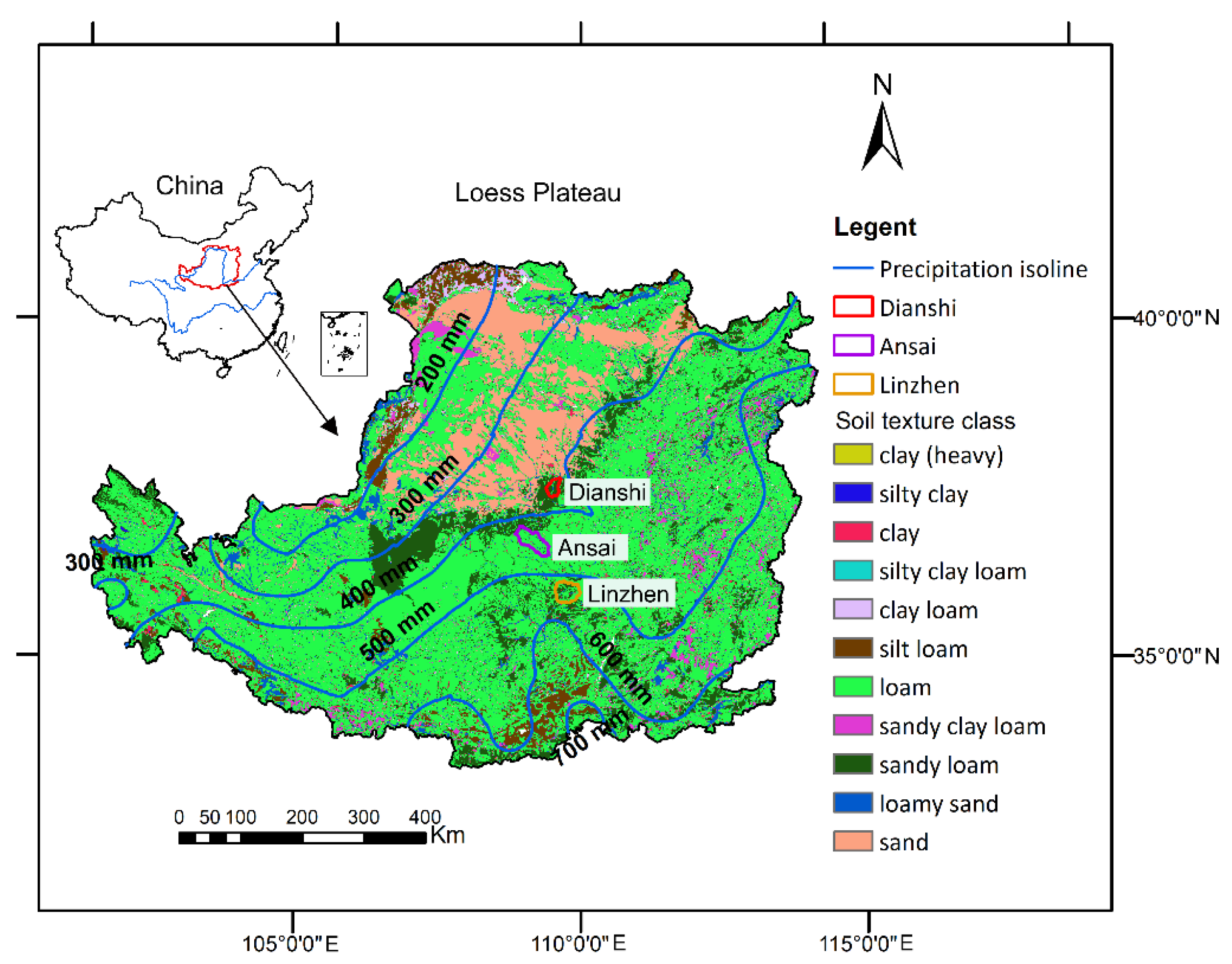
2.1. Study Area

The Loess Plateau of China is located in the middle reaches of the Yellow River basin, where there is an obvious precipitation gradient. The mean annual precipitation (MAP) gradually decreases from 700 mm in the southeast to 200 mm in the northwest, and the precipitation contours are nearly parallel in the central Loess Plateau. The vegetation types change with precipitation from dry steppe to forest-steppe and deciduous broad-leaf forest. Three independent catchments along the precipitation gradient in the central Loess Plateau were selected (Figure 1). They are controlled by the “Dianshi”, “Ansai”, and “Linzhen” hydrometric stations, where runoff and sediment are observed. The Dianshi (300 mm < MAP < 400 mm), Ansai (400 mm < MAP < 500 mm), and Linzhen (500 mm < MAP < 600 mm) watersheds are located in three precipitation zones, as illustrated in Figure 1. The study area is characterized by an arid and semiarid continental monsoon climate zone and has typical loess geomorphic landforms and eroded terrains. The soils are mainly derived from loess, a fine silt soil that is weakly resistant to erosion, and this region is considered the most eroded in the world. The soil layer of the Loess Plateau is deep, the groundwater level is mostly between 30 and 80 m, and it hardly participates in the water cycle process of the soil–vegetation–atmosphere transfer system [30]. The natural vegetation was destroyed, and considerable secondary vegetation was planted. The main forest species include Robinia pseudoacacia, Pinus tabulaeformis, and Platycladus orientalis, and the shrubs include Caragana korshinskii and Hippophae rhamnoides. Grassland communities are mainly composed of Artemisia gmelinii, Lespedeza davurica, and Stipa bungeana. Local people cultivate millet, maize, and broom corn millet in croplands. The percentage of the population dependent on agriculture (including crop farming, forestry, animal husbandry and fishery) decreased from 72.3% in 2000 to 57.9% in 2015 [31].

2.2. Data Sources

We downloaded Landsat images from the USGS [32] and generated land-use maps (30 m × 30 m) by supervised classification. We obtained meteorological data from the China Meteorological Data Service Center [33]. We obtained a DEM (30 m × 30 m) from the ASTER Global Digital Elevation Model provided by the Geospatial Data Cloud, Computer Network Information Center, Chinese Academy of Sciences [34]. The soil data were obtained from the Soil Map of China in the Harmonized World Soil Database [35].

2.3. Assessment of ESs and Land-Use Changes

The Hydrology Tool of ArcGIS 10 was used to divide the Dianshi, Ansai, and Linzhen watersheds into 240, 817, and 543 subwatersheds, respectively. We calculated and analyzed ESs at the subwatershed level in this study.

2.3.1. Soil Conservation (SEC)

Soil conservation was assessed by the “sediment delivery ratio” (SDR) model of InVEST3.3.2. First, the average amount of annual soil loss with existing vegetation was calculated by the revised universal soil loss equation (RUSLE) [36]. Then, the SDR was used to calculate the soil loss actually reaching the watershed outlet, and the SDR was directly calculated from the conductivity index using the sigmoid function [37]:
SLAx = Rx·Kx·LSx·Cx·PxSDRi
where SLAx is the annual actual soil loss that reaches the watershed outlet on pixel x; Rx is the rainfall erosivity factor on pixel x; Kx is the soil erodibility factor; LSx is the topographic factor; Cx is the cover and management factor; and Px is the engineering measures factor. SDRi is the sediment delivery ratio on pixel x.
The potential soil loss reaching the watershed outlet (SLPx) was the condition without vegetation coverage and engineering measures (Cx = 1, Px = 1):
SLPx = Rx·Kx·LSxSDRi
Finally, the actual value of the soil conservation on pixel x (SCx) was calculated as the difference between the SLAx and SLPx:
SCx = Rx·Kx·LSx(1 −·Cx·Px)SDRi
The model accuracy was evaluated by the sediment loading data at the outlet of the watershed, and the relative error between the calculated value and measured value was 3.5%, 2.3%, and 2.8% in Dianshi, Ansai, and Linzhen, respectively.

2.3.2. Water Yield (WY)

The water yield was assessed from the “Water Yield” submodel of InVEST based on the Budyko curve and annual average precipitation. The annual water yield Yx on pixel x is calculated as follows:
Yx = (1 − AETx/Px)·Px
where AETx is the annual actual evapotranspiration on pixel x and Px is the annual precipitation on pixel x. The calculations of AETx are core technology in WY estimation, which can be found in the InVEST User’s Guide [38]. The overall process is as follows: For forest, shrub, grassland, and cropland, AETx was computed by an expression of the Budyko curve proposed by Fu [39] and Zhang et al. [40]; for construction land and water bodies, AETx was directly computed from the reference evapotranspiration and has an upper limit defined by the precipitation.

2.3.3. Carbon Sequestration (TC)

Carbon storage directly depends on the carbon content of the four major carbon pools in the ecosystem, namely, aboveground biomass, underground biomass, soil carbon, and dead matter. The carbon model of InVEST can evaluate the total carbon storage by summing the four carbon pools according to the land-use maps. The data for the four major carbon pools were obtained by our field survey [41].

2.3.4. Calculation of Land-Use Changes

The ESs and land-use changes were defined as the values of the final stage minus those of the initial stage. The land use transfer matrix in a watershed was obtained by “Raster Calculator”, and the area of one land-use type transfer to another in a small watershed was calculated by the “TabulateArea” of ArcGIS 10.

2.4. Calculation of the Trade-Offs between ESs

The methods for quantifying ES trade-offs are still inadequate. The correlation coefficient [42] and root mean square error [5,29,43] are often used to calculate trade-off values. However, the correlation coefficient usually needs time series data, and the root mean square error method only reflects static trade-offs at a single given time. Thus, we proposed one indicator for quantifying ES trade-offs on the premise that trade-offs have been identified between two ESs. This indicator is based on the idea that trade-off intensity is determined by the degree of relative waxing and waning between ESs, and it is calculated as follows:
If trade-off relation can be identified between ecosystem service A and B:
T B A B = 1 2 ( ( E S A T 2 E S A T 1 E S A T 1 ) 2 + ( E S B T 2 E S B T 1 E S B T 1 ) 2 ) × 100 %
If synergy relation can be identified between ecosystem service A and B:
T B A B = 1 2 ( ( E S A T 2 E S A T 1 E S A T 1 ) 2 + ( E S B T 2 E S B T 1 E S B T 1 ) 2 ) × 100 %
where TRAB is the trade-off/synergy value between ecosystem service A and ecosystem service B; ESAT1 and ESAT2 correspond to ecosystem service A at times T1 and T2, respectively (time T1 is earlier than T2); and ESBT1 and ESBT2 correspond to ecosystem service B at times T1 and T2, respectively.
First, the ES data of the subwatersheds were prepared for the three watersheds. Second, the data in which the change direction of ESA and ESB was inverse (the increase in one coincides with the decrease in the other), indicating a trade-off between the two ESs, were selected, and TRAB was calculated by these data. Finally, the data in which ESA and ESB increased or decreased simultaneously, indicating synergy between the two ESs, were selected, and TRAB was calculated by these data to represent synergy intensity.

2.5. Statistical Analyses

Most ES trade-off and land-use change data did not conform to a normal distribution and exhibited heteroscedasticity, so robust statistical methods were employed. Spearman correlation analysis and quantile regression do not require the homogeneity of variance assumption, and they are robust to outliers [44,45] and have been widely used in macroecology. Thus, they were used to reveal the relationship between ES trade-offs and land-use changes. Quantile regression estimates a portion (certain quantiles reflecting various levels of trade-off intensity) of the response variable instead of estimating the mean of the response variable as in ordinary least squares regressions. Thus, quantile regression provides a much more complete picture of the land-use changes influencing ES trade-offs. In addition, piecewise linear regression was used to identify the thresholds of ES trade-off responses to land-use changes. In contrast to simple linear regression, piecewise linear regression explores a more detailed trend of the relationship between variables [46,47]. Redundancy analysis (RDA) was applied to reveal the effects of land-use conversion (e.g., cropland conversion to forest and grassland conversion to shrub) on ES trade-offs. A Monte Carlo permutation test based on 499 random permutations was conducted to test the significance of the marginal and conditional effects [48].
Spearman correlation analysis and quantile regression were conducted using Stata15.1. Piecewise linear regression was performed with the segmented package in the statistical software R. RDA was performed using CANOCO5.0.

3. Results and Discussion

3.1. Temporal and Spatial Variations in ESs along the Precipitation Gradient

3.1.1. Land-Use Transformation along the Precipitation Gradient

As illustrated in Table 1, cropland and grassland were the major land-use types and covered 98.7% of the Dianshi watershed in 2000, whereas the grassland, cropland, and shrub types became dominant and covered 93.7% of the area in 2018. From 2000 to 2018, cropland was mainly transformed into grassland, and grassland was mainly transformed into shrubs and cropland. Therefore, “planting grass” was the primary vegetation rehabilitation method (grassland reached 61.2% of the total area), while “afforestation” was secondary in Dianshi (forest and shrub accounted for only 17.6% of the total area).
The major land-use types were grassland and cropland (96.8%) in the Ansai watershed in 2000, whereas forest and grassland (75.8%) became the major types in 2018. The main land-use transformation characteristics in Ansai were that cropland was mainly converted to forest and grassland, grassland was mainly converted to forest and shrubland, and forest and grassland had equal areas in 2018 (approximately 37%).
The dominant land-use types were shrub, grassland, and cropland (94.8%) in the Linzhen watershed in 2000, whereas forest, shrub, and grassland (83.9%) became the dominant types in 2018. From 2000 to 2018, shrubs were mainly converted to forest, grassland was mainly converted to forest and shrubs, and cropland was mainly converted to grassland, forest, and shrubs. In brief, forested land was preferentially selected for revegetation in Linzhen.
The soil organic matter content was 0.76%, 1.18%, and 1.33% in Dianshi, Ansai, and Linzhen, respectively, before the GFGP, according to data from the Second National Soil Survey of China. The soil carbon sequestration rates were 0.43, 0.51, and 0.21 Mg ha−2·year−1 by revegetation, respectively [49]. Therefore, land-use transformation improved vegetation and soil conditions, which meant that local soil erosion would be reduced, and the agricultural production environment and farmers’ livelihoods would become increasingly better.

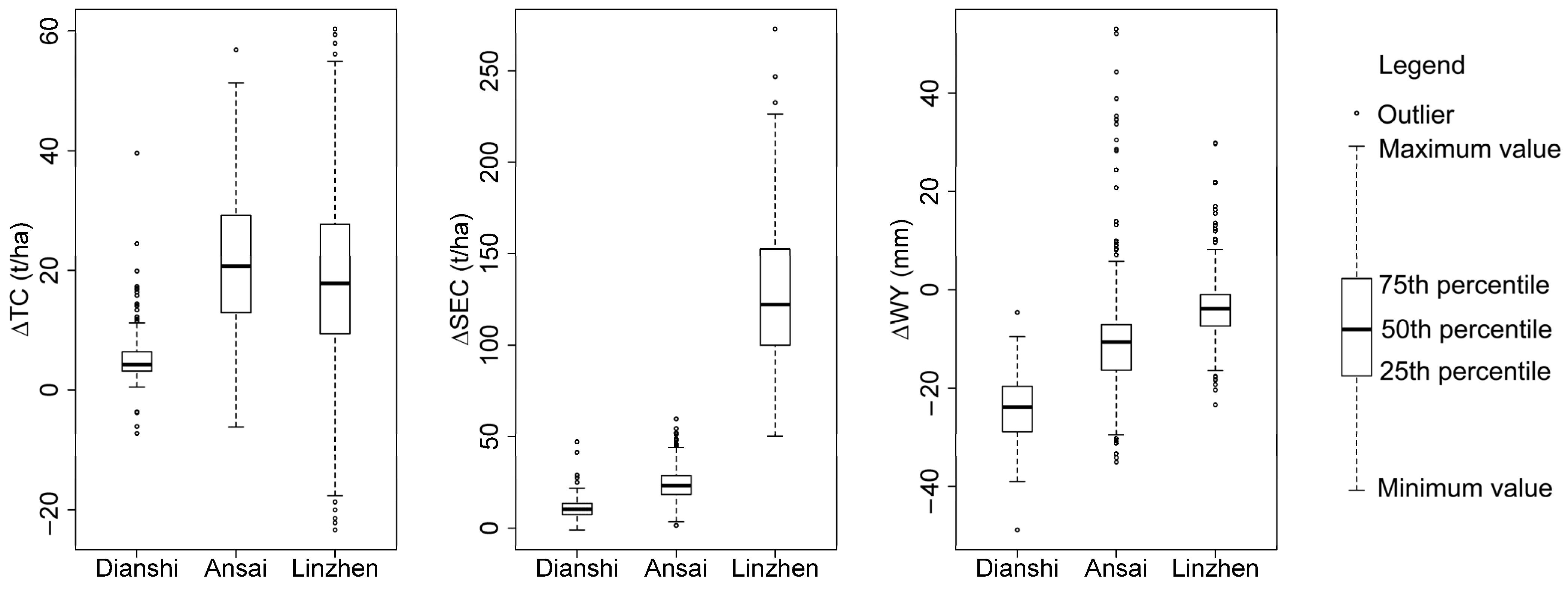
3.1.2. Changes in ESs from 2000 to 2018 along the Precipitation Gradient

As illustrated in Figure 2, TC and SEC generally increased in the three watersheds from 2000 to 2018 (most ∆TC and ∆SEC were positive values), whereas WY decreased (most ∆WY were negative values). This phenomenon indicated that TC and SEC increased at the cost of decreasing WY. Therefore, a synergistic relationship can be identified between TC and SEC as well as trade-offs between the two ESs and WY. Similar conclusions were found by some studies on the Loess Plateau of China [5,50]. The amount of variation in the ESs changed with the precipitation gradient. With regard to the mean value of ∆ESs, the increments of TC were approximative in the Ansai and Linzhen watersheds and were larger than those in Dianshi. The increment of SEC exhibited the trend of Linzhen > Ansai > Dianshi. The decrease in WY exhibited the trend of Dianshi > Ansai > Linzhen. These findings indicate that although TC and SEC were enhanced to some extent by the GFGP in Dianshi, where rainfall was the smallest, this gain was offset by the significant decrease in WY. However, there were some small watersheds where the change trends of TC and WY were opposite, especially in the Linzhen and Ansai watersheds. The reason for this is that construction land increased in these small watersheds, which reduced TC and increased WY.

3.1.3. The Correlation between Land-Use and ESs Change

The ∆TC value was significantly positively and negatively correlated with the change in forest and grassland, respectively, in the three watersheds (Table 2). ∆TC was significantly negatively correlated with the change in cropland in Dianshi and Ansai only. The correlations between ∆SEC and ∆Forest and ∆Shrub were significantly positive in Ansai and Linzhen, whereas the correlations were significantly negative with grassland change. ∆WY was significantly positively and negatively correlated with the changes in cropland and shrubs, respectively, in the three watersheds. In general, increasing forest was beneficial to TC and SEC and was not conducive to WY, whereas the influence of cropland showed the opposite trend [25,27,51]. Somewhat differently, shrubs were beneficial to TC, and grasslands were not conducive to WY in Dianshi, but the influences of shrubs and grasslands were opposite in Ansai, and this influence was not significant in Linzhen. Land-use change characteristics and rainfall differences in the three watersheds caused these phenomena.

3.2. ESs Trade-offs along the Precipitation Gradient

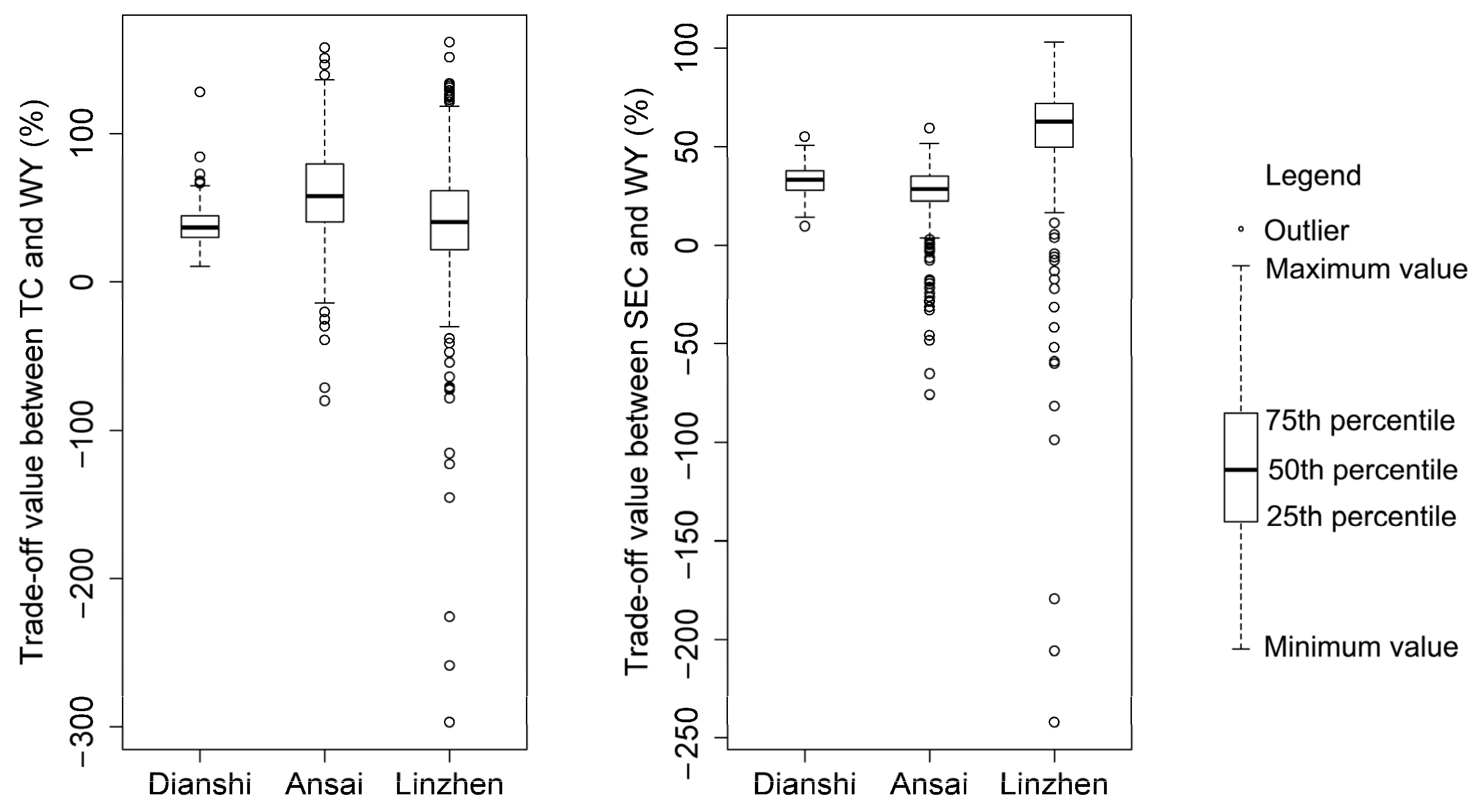
3.2.1. Comparing ES Trade-Offs in Three Precipitation Regions

As illustrated in Figure 3, the variation tendencies in the two types of trade-offs along the precipitation gradient were not consistent. The mean value of the TC-WY trade-off exhibited the trend of Ansai > Linzhen > Dianshi, and the mean value of the SEC-WY trade-off exhibited the trend of Linzhen > Dianshi > Ansai. Additionally, the variability of the ES trade-offs was large, and the variability increased with the rainfall gradient. Small watersheds with negative trade-off values appeared, indicating that synergic relationships could be identified among ESs in some small watersheds.

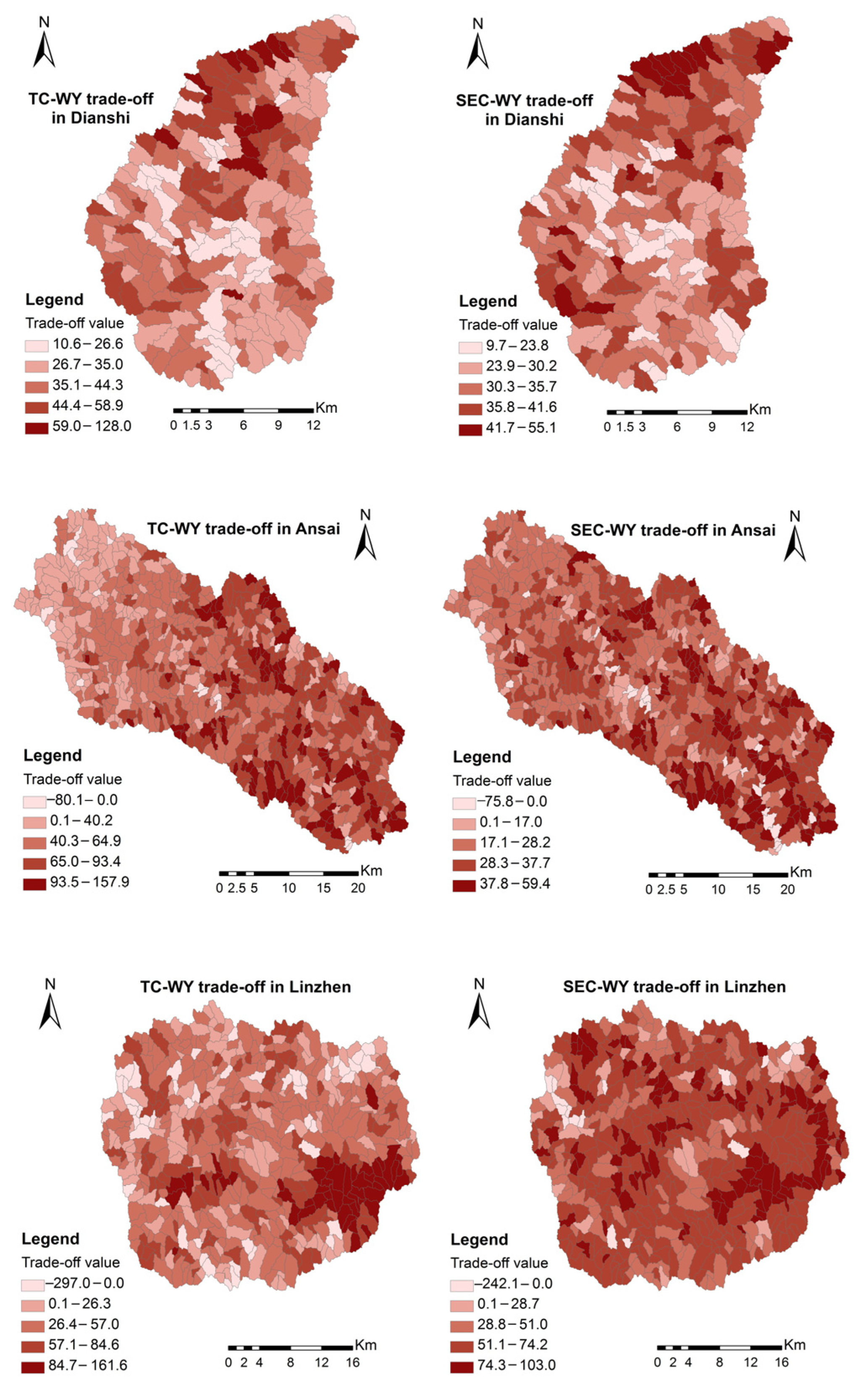
3.2.2. The Spatial Distribution of ESs Trade-Offs

As illustrated in Figure 4, the spatial distributions of the TC–WY trade-off and SEC–WY trade-off were similar in the Dianshi watershed; the high trade-off value regions were distributed in the northern watershed (lower reaches), whereas the low value regions were dispersedly distributed in the central section of the watershed. The trade-off intensity is determined by the degree of relative waxing and waning between ESs. The land-use change trends were that forest increased and cropland decreased in Dianshi, and such land-use transfers usually enhanced TC and SEC and reduced WY [23,25,27,51]; as a result, trade-off intensity increased. Using map overlay analysis between land-use and ES trade-offs, we found that the high trade-off-value areas overlapped with the areas where the increments of forest and grassland and the decrement of cropland were high. Therefore, land-use change is the direct reason for the ES trade-off.
The TC–WY and SEC–WY trade-offs decreased gradually from the southeast (lower reaches) to the northwest (upper reaches) in the Ansai watershed, which was consistent with the spatial distribution of the forest increment and in the decrements in grassland and cropland. In addition, there were small watersheds with negative trade-off values (two ESs both increased and decreased) near the main valley, indicating a synergistic relationship between the two ESs. The main reason for this was that forest and construction land slightly increased near the valley due to the flat terrain and convenient transportation; thus, the three ESs increased synchronously.
Except for some high trade-off areas assembling in the southwest, other high and low trade-off areas were fragmented and interlaced in the Linzhen watershed. The high trade-off areas coincided with the areas where grassland and cropland decreased and forests increased, whereas the low trade-off areas mainly coincided with the areas where grassland and forests increased slightly, cropland increased moderately, and shrubland decreased.

3.3. The Effects of Land-Use Changes on ESs Trade-Offs

3.3.1. The Effects of Land-Use Changes on ES Trade-Offs in Different Quantiles

Quantile regression is a method of estimating the conditional quantiles of a response variable distribution in a linear model that provides a more complete view of possible relationships between variables in ecological processes [45]. Forested land had significant positive effects (enhancing the trade-off) on TC–WY trade-offs in the three watersheds, and this positive effect exhibited the trend of Dianshi > Ansai > Linzhen (Table 3). The positive effect (regression coefficient) fluctuated by approximately 1.4 in various quantiles in the Dianshi watershed. This positive effect increased with the increase in quantiles, and it was the highest in the 80th and 90th quantiles in the Ansai and Dianshi watersheds, respectively. Forested land also had positive effects on the SEC–WY trade-off in the three watersheds, and this positive effect decreased along the precipitation gradient until the positive effect was not significant (the regression coefficients were only significant in the 30th–60th quartiles in the Linzhen watershed where the precipitation was the highest). The positive effect was highest in the 10th quantile; then, it declined with the quantile in the Dianshi watershed, and it was the highest in the 60th and 40th quantiles in the Ansai and Linzhen watersheds, respectively. Therefore, although the forest cover was low in the Dianshi watershed, the response of the trade-offs to forest cover was the strongest in this watershed, especially at a low trade-off level. This response was weaker as precipitation increased, possibly because higher rainfall can compensate for the negative effect of forest cover on water yield.
Shrubland had significant positive effects on the TC–WY trade-off, except for the 90th quantile in the Dianshi watershed, and the positive effects were larger in the Dianshi watershed than in the Ansai and Linzhen watersheds, denoting that the TC–WY trade-off in the Dianshi watershed is most sensitive to changes in shrubland. The positive effects decreased as the quantile increased in Dianshi. The effects of shrubs on the TC–WY trade-off presented a “U” pattern as the quantile increased in Ansai (shrubs intensified the trade-off first and then reduced the trade-off). The effects on the TC–WY trade-offs were enhanced as the quantile increased in Linzhen. Shrubs had significant positive effects on SEC–WY trade-offs in the three watersheds, exhibiting the trend of Dianshi > Ansai > Linzhen. The positive effects declined first and then rose as the quantile increased in the three watersheds. For low- and medium-rainfall regions, shrubland had a stronger influence on the SEC–WY trade-offs at low trade-off levels, and the influence was weaker at high trade-off levels. For high rainfall regions, the influence was stronger at high trade-off levels and weaker at moderate trade-off levels.
Grassland only had significant positive effects on TC–WY trade-offs in the 10th–30th quantiles in the Dianshi watershed, denoting that increasing grassland still exacerbated trade-offs at low trade-off levels, but the influence of grassland disappeared at moderate and high trade-off levels. In contrast, grassland significantly inhibited TC–WY trade-offs at all trade-off levels in the Ansai and Dianshi watersheds. The inhibitory effect of grassland was strongest at high trade-off levels and stronger in Ansai than in Linzhen. Grassland had significant positive effects on the SEC–WY trade-offs in the Dianshi watershed, and the effects decreased as the quantile increased. Whereas grassland significantly inhibited SEC–WY trade-offs in the Ansai watershed, the inhibitory effects were the strongest at high trade-off levels. The inhibitory effects were weaker in Linzhen than in Ansai, and the regression coefficients were statistically significant only in the 10th, 20th, and 90th quantiles. The results indicate that the water consumption of grassland could exacerbate trade-offs in low precipitation regions, especially at low trade-off levels. However, grassland could inhibit trade-offs in medium-precipitation and high-precipitation regions, so grassland could be arranged in high trade-off regions.
Cropland had inhibitory effects on the TC–WY trade-offs in the three watersheds. The regression coefficients fluctuated by approximately 0.77 in Dianshi, and the inhibitory effects were the highest at high trade-off levels in Ansai and low trade-off levels in Linzhen. Cropland also had inhibitory effects on the SEC–WY trade-offs in the three watersheds, exhibiting the general trend of Linzhen > Dianshi > Ansai. The inhibitory effects were highest at low trade-off levels in Dianshi and Linzhen and were highest at moderate trade-off levels in Ansai.

3.3.2. The Threshold Values at Which ES Trade-Offs Respond to Land-Use Changes

The influences of independent variables of different ranges on dependent variables can be revealed by piecewise linear regression, and we can use piecewise linear regression to identify the inflection point of trade-off responses to land-use changes. As illustrated in Figure 5, the intensive effect (slope of piecewise functions) of forest cover on trade-offs was higher when the increment of forested land exceeded 34.0% and 18.6% in Ansai and Linzhen, respectively, but this intensive effect was almost unchanged across the total range of the independent variable in Dianshi. Shrubland reduced the trade-offs when the shrub increased less than 8.2%, 20.1%, and −45.4% in Dianshi, Ansai, and Linzhen, respectively, whereas shrubland exacerbated trade-offs when the increment exceeded these thresholds. This phenomenon meant that the “golden mean” and limited increase in shrubs were good strategies. TC and SEC were very small, and WY was large (trade-off was intense) when there were few shrubs. In these circumstances, planting shrubs would enhance TC and SEC with low water consumption, and the trade-off would be reduced. However, the sustained planting of shrubs would reverse the relative size of ESs and strengthen the trade-off due to water deficiency. Therefore, although the water consumption of shrubs was less than that of forests, the water consumption of shrubs still cannot be ignored. Grassland reduced the trade-offs when the grassland increased less than 16.5% in Dianshi, but grassland exacerbated trade-offs when the increment exceeded the threshold, which was caused by very low rainfall in Dianshi. Generally, it is more reasonable to establish grassland in arid regions [5,52] because the water consumption of grassland is usually lower and grassland can provide higher WY and maintain other ESs at a relatively high level [5,25,27,53]. However, too much grassland may exceed the soil-water carrying capacity for vegetation, especially in low rainfall areas such as the Dianshi watershed. Grassland reduced trade-offs in Ansai, and the inhibitory action was relatively stable across the total range of grassland change. Grassland reduced trade-offs in the initial stage of grassland change in the Linzhen watershed, whereas grassland slightly enhanced trade-offs when the increment of grassland exceeded −16.9%. The comprehensive analysis of the threshold value, segmental slope, and land-use proportions of the initial period (2000) showed that to control ES trade-offs, forest needed to be limited, especially in the Dianshi and Ansai watersheds, and shrubland proportions needed to be controlled at 8.5% and 21.6% in Dianshi and Ansai, respectively, whereas grassland proportions needed to be controlled at 58.0% in Dianshi. In addition, Wang et al. [29] also calculated the trade-offs between soil moisture and soil organic carbon, total nitrogen, and species richness at a single time point in the Loess Plateau of China, and the inflection point of the trade-offs responding to the precipitation gradient was identified.

3.3.3. The Effects of Land-Use Transformation on ESs Trade-Offs

The conversion of cropland and grassland to forests and shrubland was the main reason for the trade-off increase in the three watersheds, but which land-use transformations could reduce the trade-offs were different in the three watersheds (Table 4). Grassland conversion to cropland, cropland remaining unchanged, and grassland and cropland conversion to construction land could reduce the trade-offs in the Dianshi watershed. Grassland remaining unchanged, cropland conversion to grassland and construction land, and grassland conversion to construction land could reduce the trade-offs in the Ansai watershed. Forest and shrubland conversion to cropland could reduce the trade-offs in the Linzhen watershed. Therefore, it is necessary to ensure a certain proportion of cropland in low precipitation regions as well as certain grassland in medium precipitation regions, and forested land and shrubland need to be reduced appropriately in the high precipitation region.

3.4. Recommendations of ES Regulation for Various Precipitation Regions

Forests are propitious to carbon sequestration, soil and water conservation, climatic regulation, and atmospheric purification, but they are not propitious to water yield, especially in arid regions [11,50,54,55]. However, the function of cropland is contrary to that of forested land [25,27]. As a land-use type, grassland is a compromise [5,27]. Thus, regulating the proportions of several land use types can realize the balance of various ESs and reduce their trade-offs. For the low precipitation region (Dianshi watershed), the balancing of trade-offs could be achieved by restricting forest, shrub, and grassland, increasing cropland properly in low trade-off areas, while keeping most of the current cropland unchanged, converting grassland to cropland reasonably, and converting grassland and cropland to construction land moderately in high trade-off areas. For the medium precipitation region (Ansai watershed), restricting shrubs in low trade-off areas, restricting forests, and increasing shrubs, grasslands, and croplands appropriately in high trade-off areas could increase the balance in trade-offs, and specific land-use transformations such as keeping current grasslands unchanged, converting cropland to grassland and construction land, and slightly converting grassland to construction land could also improve the balance. For high precipitation regions (Linzhen watershed), increasing cropland in low trade-off areas, restricting forested land and shrubland, and increasing grassland and cropland in high trade-off areas could help achieve balance. The main land-use transformation tactic is the conversion of forest and shrubs to cropland. In addition, some useful measures can be implemented in the whole study area, such as enhancing the quality of the current vegetation, improving the community structure, increasing biodiversity, tending forests and shrubs, rational grazing in grassland, employing conservation tillage, developing water-saving agriculture, and applying forest-crop intercropping.

3.5. The Limitation of the Methods and Results

The InVEST model was used to calculate ESs in this study. Depending on many advantages, such as simplicity and convenience, flexible operation, and strong spatial expression ability of output results, the InVEST model is widely applied to ecosystem management and decision making. However, the principles of calculations are simplified for many ESs. For example, errors in the empirical parameters of the revised universal soil loss equation (RUSLE) will therefore have a large effect on SEC predictions; WY calculation is based on annual averages, which neglect extremes; TC is calculated by the summation of the carbon content of the four major carbon pools, and ecological processes are ignored. Other important issues are that biophysical parameters are too dependent on land-use types, but land-use maps cannot reveal the differences within the same land-use type. Despite this, the InVEST model is a powerful tool to map and value ecosystem services at watershed and regional scales.
ESs are affected by land use, climate, soil, topography, and many other factors. Land use influences carbon sequestration [56] and soil conservation directly [57], and it also influences water yield by hydrologic processes [58]. Similarly, precipitation is the key factor for carbon sequestration [59], soil conservation [60], and water yield [61]. Soil properties affect plant growth [62], soil erosion [63], and hydrologic processes [64], and they are also important factors for these three ESs. In this study, the effects of land use on ESs trade-offs were analyzed in three precipitation regions, and other factors, such as soil, were not introduced, which would limit the results and corresponding management recommendations. Nevertheless, vegetation and soil exhibit zonal distributions across precipitation gradients in the Loess Plateau of China [14]. The current geographical landscape is formed by the collaborative evolution of many natural geographical factors. The regional differentiation of ESs across precipitation gradients implied differentiation across other environmental gradients. Therefore, we only employ land use and precipitation to study ESs trade-offs. Although there are certain limitations, the conclusions are reliable, and it is propitious to apply the results in practice.

4. Conclusions

From 2000 to 2018, TC and SEC were enhanced, but WY decreased in the three watersheds, and a trade-off relation can be identified between these two ESs and WY. The effects of forests on the trade-offs were positive in the three watersheds, and the main effects exhibited decreasing, increasing, and increasing trends as trade-off intensity increased in Dianshi, Ansai, and Linzhen, respectively. The positive effect of shrubs on TC–WY trade-offs exhibited a decreasing trend, a “U” pattern, and an increasing trend as the trade-off intensity increased in Dianshi, Ansai, and Linzhen, respectively; these effects on the SEC–WY trade-offs first declined and then rose in the three watersheds. Grassland exacerbated trade-offs in Dianshi, whereas it reduced trade-offs in Ansai and Linzhen. Regulating land-use proportions can realize the balance of three ESs and reduce their trade-offs. For Dianshi, we can restrict forest, shrub, and grassland and increase cropland properly. For Ansai, we can restrict shrubs in low trade-off areas, and we can also restrict forests and increase shrubs, grasslands, and croplands appropriately in high trade-off areas. For Linzhen, we can increase cropland in low trade-off areas, and we can restrict forest and shrub but increase grassland and cropland in high trade-off areas.

Author Contributions

Methodology, writing—original draft preparation, Q.F.; writing—review and editing, supervision, S.D.; investigation and data curation, B.D. All authors have read and agreed to the published version of the manuscript.

Funding

This research was funded by the National Natural Science Foundation of China (No. 41501201) and the Fundamental Research Program of Shanxi Province (No. 20210302123481).

Institutional Review Board Statement

Not applicable.

Informed Consent Statement

Not applicable.

Data Availability Statement

The data presented in this study are available on request from the corresponding author.

Conflicts of Interest

The authors declare no conflict of interest.

References

  1. Costanza, R.; D’Arge, R.; Groot, R.D.; Farber, S.; Grasso, M.; Hannon, B. The value of the world’s ecosystem services and natural capital. Nature 1997, 25, 3–15. [Google Scholar] [CrossRef]
  2. Gentry, R.R.; Alleway, H.K.; Bishop, M.J. Exploring the potential for marine aquaculture to contribute to ecosystem services. Rev. Aquac. 2020, 12, 499–512. [Google Scholar] [CrossRef] [Green Version]
  3. Millennium Ecosystem Assessment. Ecosystem and Human Well-Being; Island Press: Washington, DC, USA, 2005; pp. 137–142. [Google Scholar]
  4. Bennett, E.M.; Peterson, G.D.; Gordon, L.J. Understanding relationships among multiple ecosystem services. Ecol. Lett. 2009, 12, 1394. [Google Scholar] [CrossRef]
  5. Wu, X.; Wang, S.; Fu, B.; Liu, Y.; Zhu, Y. Land use optimization based on ecosystem service assessment: A case study in the Yanhe watershed. Land Use Policy 2018, 72, 303–312. [Google Scholar] [CrossRef]
  6. Karimi, J.D.; Corstanje, R.; Harris, J.A. Understanding the importance of landscape configuration on ecosystem service bundles at a high resolution in urban landscapes in the UK. Landsc. Ecol. 2021, 36, 2007–2024. [Google Scholar] [CrossRef]
  7. Lu, N.; Liu, L.; Yu, D.; Fu, B. Navigating trade-offs in the social-ecological systems. Curr. Opin. Environ. Sustain. 2011, 48, 77–84. [Google Scholar] [CrossRef]
  8. Agol, D.; Reid, H.; Crick, F. Ecosystem-based adaptation in Lake Victoria Basin; synergies and trade-offs. R. Soc. Open Sci. 2021, 8, 201847. [Google Scholar] [CrossRef] [PubMed]
  9. Knapp, A.K.; Fay, P.A.; Blair, J.M. Rainfall variability, carbon cycling, and plant species diversity in a mesic grassland. Science 2002, 298, 2201–2205. [Google Scholar] [CrossRef] [PubMed] [Green Version]
  10. Meier, I.C.; Leuschner, C. Nutrient dynamics along a precipitation gradient in European beech forests. Biogeochemistry 2014, 120, 51–69. [Google Scholar] [CrossRef]
  11. Feng, X.; Fu, B.; Lü, N.; Zeng, Y.; Wu, B. How ecological restoration alters ecosystem services: An analysis of carbon sequestration in China’s Loess Plateau. Sci. Rep. 2012, 3, 2846. [Google Scholar] [CrossRef] [PubMed]
  12. Li, T.; Ren, B.; Wang, D. Spatial variation in the storages and age-related dynamics of forest carbon sequestration in different climate zones-evidence from black locust plantations on the Loess Plateau of China. PLoS ONE 2015, 10, e0121862. [Google Scholar] [CrossRef] [Green Version]
  13. Zhang, J.; Xu, B.; Li, M. Diversity of communities dominated by Glycyrrhiza uralensis, an endangered medicinal plant species, along a precipitation gradient in China. Bot. Stud. 2011, 52, 493–501. [Google Scholar]
  14. Zhang, Y.; Huang, M.; Lian, J. Spatial distributions of optimal plant coverage for the dominant tree and shrub species along a precipitation gradient on the central Loess Plateau. Agric. For. Meteorol. 2015, 206, 69–84. [Google Scholar] [CrossRef]
  15. Shi, S.; Li, Z.; Wang, H.; Wu, X.; Wang, S.; Wang, X. Comparative analysis of annual rings of perennial forbs in the Loess Plateau, China. Dendrochronologia. 2016, 38, 82–89. [Google Scholar] [CrossRef]
  16. Jia, X.; Shao, M.; Yu, D. Spatial variations in soil-water carrying capacity of three typical revegetation species on the Loess Plateau, China. Agric. Ecosyst. Environ. 2019, 273, 25–35. [Google Scholar] [CrossRef] [Green Version]
  17. Cao, Y.; Li, Y.; Chen, Y. Non-structural carbon, nitrogen, and phosphorus between black locust and Chinese pine plantations along a precipitation gradient on the Loess Plateau, China. Trees 2018, 32, 835–846. [Google Scholar] [CrossRef]
  18. Du, C.; Gao, Y. Opposite patterns of soil organic and inorganic carbon along a climate gradient in the alpine steppe of northern Tibetan Plateau. Catena 2020, 186, 104366. [Google Scholar] [CrossRef]
  19. Zhang, X.; Song, Z.; Hao, Q. Storage of soil phytoliths and phytolith-occluded carbon along a precipitation gradient in grasslands of northern China. Geoderma 2020, 364, 114–200. [Google Scholar] [CrossRef]
  20. Wang, X.; Lü, X.; Dijkstra, F.; Zhang, H.; Han, X. Changes of plant N: P stoichiometry across a 3000-km aridity transect in grasslands of northern China. Plant Soil 2019, 443, 107–119. [Google Scholar] [CrossRef]
  21. Li, S.; Liang, W.; Zhang, W.; Liu, Q. Response of soil moisture to hydro-meteorological variables under different precipitation gradients in the yellow river basin. Water Resour. Manag. 2016, 30, 1867–1884. [Google Scholar] [CrossRef]
  22. Li, Z.; Coles, A.; Xiao, J. Groundwater and streamflow sources in China’s Loess Plateau on catchment scale. Catena 2019, 181, 104075. [Google Scholar] [CrossRef]
  23. Jia, X.; Fu, B.; Feng, X.; Hou, G.; Liu, Y.; Wang, X. The tradeoff and synergy between ecosystem services in the Grain-for-Green areas in Northern Shaanxi, China. Ecol. Indic. 2014, 43, 103–113. [Google Scholar] [CrossRef]
  24. Zheng, Z.; Fu, B.; Hu, H.; Sun, G. A method to identify the variable ecosystem services relationship across time: A case study on Yanhe Basin, China. Landsc. Ecol. 2014, 29, 1689–1696. [Google Scholar] [CrossRef]
  25. Feng, Q.; Zhao, W.W.; Fu, B.J.; Ding, J.Y.; Wang, S. Ecosystem service trade-offs and their influencing factors: A case study in the Loess Plateau of China. Sci. Total Environ. 2017, 607–608, 1250–1263. [Google Scholar] [CrossRef] [PubMed]
  26. Hu, H.; Fu, B.; Lü, Y.; Zheng, Z. SAORES: A spatially explicit assessment and optimization tool for regional ecosystem services. Landsc. Ecol. 2014, 30, 547–560. [Google Scholar] [CrossRef] [Green Version]
  27. Feng, Q.; Zhao, W.; Hu, X.; Liu, Y.; Daryanto, S.; Cherubini, F. Trading-off ecosystem services for better ecological restoration: A case study in the Loess Plateau of China. J. Clean. Prod. 2020, 257, 120469. [Google Scholar] [CrossRef]
  28. Lu, N.; Fu, B.; Jin, T.; Chang, R. Trade-off analyses of multiple ecosystem services by plantations along a precipitation gradient across Loess Plateau landscapes. Landsc. Ecol. 2014, 29, 1697–1708. [Google Scholar] [CrossRef]
  29. Wang, C.; Wang, S.; Fu, B.; Li, Z.; Wu, X.; Tang, Q. Precipitation gradient determines the tradeoff between soil moisture and soil organic carbon, total nitrogen, and species richness in the Loess Plateau, China. Sci. Total Environ. 2017, 575, 1538. [Google Scholar] [CrossRef]
  30. Shao, M.; Wang, Y.; Jia, X. Ecological construction and soil desiccation on the Loess Plateau of China. Bull. Chin. Acad. Sci. 2015, 30, 257–264. (In Chinese) [Google Scholar]
  31. Wu, X.; Wang, S.; Fu, B.; Feng, X.; Chen, Y. Socio-ecological changes on the loess plateau of China after grain to green program. Sci. Total Environ. 2019, 678, 565–573. [Google Scholar] [CrossRef] [PubMed]
  32. Landsat Images. Available online: http://glovis.usgs.gov/ (accessed on 21 May 2020).
  33. Meteorological Data. Available online: http://data.cma.cn/ (accessed on 10 April 2020).
  34. Digital Elevation Model. Available online: http://www.gscloud.cn/ (accessed on 29 January 2020).
  35. Harmonized World Soil Database. Available online: http://www.crensed.ac.cn/ (accessed on 18 June 2020).
  36. Renard, K.; Foster, G.; Weesies, G.; McCool, D.; Yoder, D. Predicting Soil Erosion by Water: A Guide to Conservation Planning with the Revised Universal Soil Loss Equation (RUSLE); USDA, Agricultural Handbook Number 703; U.S. Government Printing Office: Washington, DC, USA, 1997; pp. 1–18. [Google Scholar]
  37. Vigiak, O.; Borselli, L.; Newham, L.; Mcinnes, J.; Roberts, A. Comparison of conceptual landscape metrics to define hillslope-scale sediment delivery ratio. Geomorphology 2012, 138, 74–88. [Google Scholar] [CrossRef]
  38. Sharp, R.; Tallis, H.T.; Ricketts, T.; Guerry, A.D.; Wood, S.A.; Chaplin-Kramer, R. InVEST + VERSION + User’s Guide; The Natural Capital Project, Stanford University, University of Minnesota, The Nature Conservancy, and World Wildlife Fund: Palo Alto, CA, USA, 2016; pp. 115–120. [Google Scholar]
  39. Fu, B. On the calculation of the evaporation from land surface. Sci. Atmos. Sin. 1981, 5, 23–31. [Google Scholar]
  40. Zhang, L.; Hickel, K.; Dawes, W.R.; Chiew, F.H.S.; Western, A.W.; Briggs, P.R. A rational function approach for estimating mean annual evapotranspiration. Water Resour. Res. 2004, 40, 89–97. [Google Scholar] [CrossRef]
  41. Feng, Q. Ecosystem Services Trade-Offs in the Loess Hilly and Gully Region. Ph.D. Thesis, Beijing Normal University, Beijing, China, 2018. (In Chinese). [Google Scholar]
  42. Li, B.; Chen, N.; Wang, Y.; Wang, W. Spatio-temporal quantification of the trade-offs and synergies among ecosystem services based on grid-cells: A case study of Guanzhong Basin, NW China. Ecol. Indic. 2018, 94, 246–253. [Google Scholar] [CrossRef]
  43. Bradford, J.B.; D’Amato, A.W. Recognizing trade-offs in multi-objective land management. Front. Ecol. Environ. 2012, 10, 210–216. [Google Scholar] [CrossRef] [Green Version]
  44. Xiao, C.; Ye, J.; Esteves, R.M. Using Spearman’s correlation coefficients for exploratory data analysis on big dataset. Concurr. Comput. 2016, 28, 3866–3878. [Google Scholar] [CrossRef]
  45. Cade, B.S.; Noon, B.R. A gentle introduction to quantile regression for ecologists. Front. Ecol. Environ. 2003, 1, 412–420. [Google Scholar] [CrossRef]
  46. Toms, J.D.; Lesperance, M.L. Piecewise regression: A tool for identifying ecological thresholds. Ecology 2003, 84, 2034–2041. [Google Scholar] [CrossRef]
  47. Peng, J.; Tian, L.; Liu, Y.; Zhao, M.; Hu, Y.; Wu, J. Ecosystem services response to urbanization in metropolitan areas: Thresholds identification. Sci. Total Environ. 2017, 607–608, 706–714. [Google Scholar] [CrossRef]
  48. Šmilauer, P.; Lepš, J. Multivariate Analysis of Ecological Data Using Canoco 5; Cambridge University Press: New York, NY, USA, 2014; pp. 50–69. [Google Scholar]
  49. Deng, L. Responsing Mechanism of Ecosystem Carbon Sequestration Benefits to Vegetation Restoration on the Loess Plateau of China; Northwest A&F University: Yangling, China, 2014. (In Chinese) [Google Scholar]
  50. Lü, Y.; Fu, B.; Feng, X.; Zeng, Y.; Liu, Y.; Chang, R.; Sun, G.; Wu, B. A policy-driven large scale ecological restoration: Quantifying ecosystem services changes in the Loess Plateau of China. PLoS ONE 2012, 7, e31782. [Google Scholar] [CrossRef]
  51. Yang, S.; Zhao, W.; Liu, Y. Influence of land use change on the ecosystem service trade-offs in the ecological restoration area: Dynamics and scenarios in the Yanhe watershed, China. Sci. Total Environ. 2018, 644, 556–566. [Google Scholar] [CrossRef] [PubMed]
  52. Chisholm, R.A. Trade-offs between ecosystem services: Water and carbon in a biodiversity hotspot. Ecol. Econ. 2010, 69, 1973–1987. [Google Scholar] [CrossRef]
  53. Mark, A.F.; Dickinson, K.J.M. Maximizing water yield with indigenous non-forest vegetation: A New Zealand perspective. Front Ecol. Environ. 2008, 6, 25–34. [Google Scholar] [CrossRef]
  54. Fu, B.J.; Liu, Y.; Lü, Y.H.; He, C.S.; Zeng, Y.; Wu, B.F. Assessing the soil erosion control service of ecosystems change in the Loess Plateau of China. Ecol. Complex. 2011, 8, 284–293. [Google Scholar] [CrossRef]
  55. Wang, S.; Fu, B. Trade-offs between forest ecosystem services. For. Policy. Econ. 2013, 26, 145–146. [Google Scholar] [CrossRef]
  56. Zhang, F.; Xu, N.; Wang, C.; Wu, F.; Chu, X. Effects of land use and land cover change on carbon sequestration and adaptive management in Shanghai, China. Phys. Chem. Earth. 2020, 120, 102948. [Google Scholar] [CrossRef]
  57. Napoli, M.; Altobelli, F.; Orlandini, S. Effect of land set up systems on soil losses. Ital. J. Agron. 2020, 15, 306–314. [Google Scholar] [CrossRef]
  58. Khorchani, M.; Nadal-Romero, E.; Lasanta, T.; Tague, C. Carbon sequestration and water yield tradeoffs following restoration of abandoned agricultural lands in Mediterranean mountains. Environ. Res. 2021, 10, 112203. [Google Scholar] [CrossRef] [PubMed]
  59. Hein, C.J.; Usman, M.; Eglinton, T.I.; Haghipour, N.; Galy, V.V. Millennial-scale hydroclimate control of tropical soil carbon storage. Nature 2020, 581, 63–66. [Google Scholar] [CrossRef] [PubMed]
  60. Fang, H. Responses of runoff and soil loss to rainfall regimes and soil conservation measures on cultivated slopes in a hilly region of Northern China. Int. J. Environ. Res. Public Health 2021, 18, 2102. [Google Scholar] [CrossRef] [PubMed]
  61. Lian, X.H.; Qi, Y.; Wang, H.W.; Zhang, J.; Yang, R. Assessing changes of water yield in Qinghai Lake watershed of China. Water 2020, 12, 11. [Google Scholar] [CrossRef] [Green Version]
  62. Afonso, S.; Arrobas, M.; Rodrigues, M.A. Soil and plant analyses to diagnose Hop fields irregular growth. J. Soil Sci. Plant Nutr. 2020, 20, 1999–2013. [Google Scholar] [CrossRef]
  63. Hao, H.X.; Qin, J.H.; Sun, Z.X.; Guo, Z.L.; Wang, J.G. Erosion-reducing effects of plant roots during concentrated flow under contrasting textured soils. Catena 2021, 203, 105378. [Google Scholar] [CrossRef]
  64. Bonetti, S.; Wei, Z.W.; Or, D. A framework for quantifying hydrologic effects of soil structure across scales. Commun. Earth Environ. 2021, 2, 107. [Google Scholar] [CrossRef]
Figure 1. The location of the study area (soil texture class was obtained from the soil map of China in the Harmonized World Soil Database).
Sustainability 13 13306 g001
Figure 2. Boxplot of ES changes in three watersheds (∆TC, ∆SEC, and ∆WY represent ES changes from 2000–2018).
Sustainability 13 13306 g002
Figure 3. Boxplot of ESs trade-offs in three watersheds.
Sustainability 13 13306 g003
Figure 4. The spatial distribution of ES trade-offs in the three watersheds.
Sustainability 13 13306 g004
Figure 5. The threshold value at which ES trade-offs respond to land-use changes (trade-off value of ordinate label was the mean value of TC–WY and SEC–WY trade-offs).
Sustainability 13 13306 g005
Table 1. Land-use transformation matrix from 2000 to 2018 (%).
FoL in 2018ShL in 2018GrA in 2018CrO in 2018CoL in 2018WaB in 2018Total in 2000
DianshiFoL in 20000.110.090.410.040.010.000.66
ShL in 20000.120.060.080.010.000.000.27
GrA in 20001.186.4128.035.010.620.2341.47
CrO in 20002.926.7232.5514.070.910.0357.20
CoL in 20000.000.010.030.020.080.000.14
WaB in 20000.000.010.120.040.000.090.27
Total in 20184.3413.2961.2219.191.620.35
Change from 2000 to 20183.6813.0219.74−38.011.480.08
AnsaiFoL in 20000.960.120.270.100.050.011.51
ShL in 20000.590.210.540.090.030.001.46
GrA in 200020.016.9722.893.631.070.2554.82
CrO in 200017.365.4613.094.821.260.0442.03
CoL in 20000.040.000.010.040.070.000.16
WaB in 20000.010.000.010.000.000.000.03
Total in 201838.9612.7736.828.672.470.30
Change from 2000 to 201837.4511.31−18.00−33.352.310.27
LinzhenFoL in 20002.371.750.500.300.050.004.97
ShL in 200023.3512.447.144.340.890.0148.18
GrA in 200010.109.552.971.910.400.0825.02
CrO in 20004.753.435.456.781.070.1421.61
CoL in 20000.000.020.010.030.030.000.09
WaB in 20000.000.010.010.090.000.020.12
Total in 201840.5827.2016.0813.452.440.25
Change from 2000 to 201835.61−20.98−8.94−8.162.350.13
FoL: forestland, ShL: shrubland, GrA: grassland, CrO: cropland, CoL: construction land, WaB: water body. An example to explain the meaning of the transformation matrix: Figure 6.41 in the second column of the third row means that 6.41% of grassland in 2000 was changed to shrubland in 2018.
Table 2. Spearman correlation analysis between land use and ES change.
∆ESsWatershed∆Forest∆Shrub∆Grassland∆Cropland
∆TCDianshi0.730 **0.402 **−0.291 **−0.410 **
Ansai0.922 **−0.167 **−0.723 **−0.262 **
Linzhen0.891 **−0.002−0.445 **−0.02
∆SECDianshi−0.0140.0870.035−0.157 *
Ansai0.299 **0.076*−0.169 **−0.330 **
Linzhen0.196 **0.237 **−0.351 **0.063
∆WYDianshi−0.006−0.145 *−0.527 **0.852 **
Ansai−0.530 **−0.099 **0.412 **0.203 **
Linzhen−0.082−0.276 **−0.0230.917 **
The asterisks * and ** indicate p < 0.05 and p < 0.01 respectively.
Table 3. Quantile regression between land-use changes and ES trade-offs.
Land-UseQuantileTC–WY Trade-OffsSEC–WY Trade-Offs
DianshiAnsaiLinzhenDianshiAnsaiLinzhen
Forest10th1.485 **1.061 **0.614 **0.411 **0.168 **0.051
20th1.366 **1.099 **0.658 **0.271 **0.168 **0.089
30th1.378 **1.173 **0.648 **0.296 **0.225 **0.126 **
40th1.395 **1.186 **0.695 **0.316 **0.257 **0.135 **
50th1.453 **1.213 **0.724 **0.263 **0.254 **0.092 **
60th1.374 **1.286 **0.81 **0.256 **0.287 **0.07 **
70th1.411 **1.316 **0.816 **0.307 **0.284 **0.045
80th1.378 **1.322 **0.96 **0.273 **0.286 **0.032
90th1.309 **1.296 **1.125 **0.232 *0.258 **0.004
Shrub10th0.801 **0.231 *0.0160.362 **0.282 **0.083 **
20th0.687 **0.0410.0240.3 **0.211 **0.078 **
30th0.668 **−0.149 *0.0170.273 **0.213 **0.086 **
40th0.668 **−0.281 **0.0660.264 **0.173 **0.079 **
50th0.644 **−0.313 **0.082 *0.238 **0.183 **0.057 **
60th0.6 **−0.327 *0.109 *0.186 **0.183 **0.055 **
70th0.552 **−0.2040.151 **0.162 **0.125 **0.056 **
80th0.455 **−0.1790.235 **0.1510.12 *0.085 **
90th0.2840.0090.376 **0.1850.183 **0.095 **
Grassland10th0.282 **−0.716 **−0.227 **0.441 **−0.09 **−0.12 **
20th0.221 **−0.86 **−0.287 **0.382 **−0.118 **−0.072 **
30th0.194 *−0.942 **−0.295 **0.324 **−0.171 **−0.046
40th0.081−1.004 **−0.308 **0.286 **−0.199 **−0.046
50th0.009−1.038 **−0.343 **0.251 **−0.222 **−0.034
60th−0.04−1.075 **−0.331 **0.175 **−0.228 **−0.024
70th−0.152−1.125 **−0.381 **0.139 *−0.268 **−0.017
80th−0.155−1.152 **−0.454 **0.112 *−0.265 **−0.014
90th−0.158−1.185 **−0.511 **0.125 *−0.297 **−0.035 *
Cropland10th−0.837 **−0.561 **−0.493 **−0.637 **−0.256 **−0.726 **
20th−0.742 **−0.719 **−0.344 **−0.59 **−0.308 **−0.667 **
30th−0.717 **−0.789 **−0.302 **−0.613 **−0.35 **−0.664 **
40th−0.738 **−0.887 **−0.317 **−0.621 **−0.353 **−0.644 **
50th−0.753 **−0.955 **−0.317 **−0.609 **−0.362 **−0.564 **
60th−0.735 **−0.983 **−0.281 *−0.581 **−0.403 **−0.574 **
70th−0.724 **−1.047 **−0.17−0.553 **−0.403 **−0.551 **
80th−0.791 **−1.084 **−0.114−0.538 **−0.373 **−0.536 **
90th−0.866 **−1.207 **−0.164−0.476 **−0.361 **−0.569 **
The asterisks * and ** indicate p < 0.05 and p < 0.01 respectively.
Table 4. Marginal (Marg, %) and conditional effects (Cond, %) of land-use transformation (LUT) on ES trade-offs (mean value of TC–WY and SEC–WY trade-offs).
Dianshi WatershedAnsai WatershedLinzhen Watershed
LUTMargLUTCondLUTMargLUTCondLUTMargLUTCond
LCrO-FoL43.1LCRO-FOL43.1LCRO-FOL45.9LCRO-FOL45.9LShL-CrO43.4LShL-CrO43.4
LGrA-FoL36.2LGrA-CrO22.6LGrA-FoL43.7LCrO-CoL19.7LFoL-CrO35.3LFoL-CrO14.5
LGrA-CrO34.3LCrO-ShL9.6LGrA-GrA20.3LGrA-FoL7.5LGrA-FoL22.6LGrA-FoL10.8
LCrO-CrO28.2LCrO-GrA7.1LCrO-GrA19.1LGrA-ShL7.3LCRO-FOL6.6LCRO-FOL11.3
LCrO-ShL12.6 LCrO-CoL12.1LGrA-CoL5.5LGrA-ShL6.6
LGrA-CoL7.9 LGrA-CoL9.9
LCrO-CoL6.3 LShL-GrA5.9
LGrA-GrA5.0
FoL: forestland, ShL: shrubland, GrA: grassland, CrO: cropland, CoL: construction land, WaB: water body. LCrO-FoL represents the land-use type change from cropland to forestland. Land-use transformation with gray shadow represents negative effects on trade-offs, and others represent positive effects.
Publisher’s Note: MDPI stays neutral with regard to jurisdictional claims in published maps and institutional affiliations.

