Study of Vortex Systems as a Method to Weakening the Urban Heat Islands within the Financial District in Large Cities

Abstract

This paper presents a new concept called the urban vortex system (UVS). The UVS couples a vortex generator (V.G.) that produces updraft by artificial vortex and a vortex stability zone (VSZ) consisting of an assembly of four buildings acting as a chimney. Through this system, a stable, upward vortex flow can be generated. The Reynolds Averaged Navier–Stokes (RANS) simulation was carried out to investigate the flow field in the UVS. The Renormalized Group (RNG) k–ε turbulent model was selected to solve the complex turbulent flow. Validation of the numerical results was achieved by making a comparison with the large-size experimental model. The results reported that a steady-state vortex could be formed when a vapor-air mixture at 2 m/s and 450 K enters the vortex generator. This vortex presented a maximum negative central pressure of −6.81 Pa and a maximum velocity of 5.47 (m/s). Finally, the similarity method found four dimensionless parameters, which allowed all the flow characteristics to be transported on a large scale. The proposed large-scale UVS application is predicted to be capable, with have a maximum power of 2 M.W., a specific work of 3 kJ/kg, buildings 200-m high, and the ability to generate winds of 6.1 m/s (20 km/h) at 200 m up to winds of 1.5 m/s (5 km/h) at 400 m. These winds would cause the rupture of the gas capsule of the heat island phenomenon. Therefore, the city would balance its temperature with that of the surrounding rural areas.

1. Introduction

In medium and large cities, the urban environmental temperature is higher than in the rural areas. This effect is known as Urban Heat Island (UHI) [1]. It results from the growing proportion of the national population of a country moving to live in urban areas, which demands an increase in electrical power demand, water, and fuel consumption. These demands are reflected in an increase in greenhouse gas emissions that causes environmental degradation [2].

Adverse effects from UHI development are generally classified into people and (micro) climates [3]. The increase of UHI intensity can negatively affect the citizens’ well-being in several ways, such as thermoregulatory system damages [4]. Intense heatwaves can elevate the demands for air conditioning in buildings, especially among people who are more sensitive to heat (namely the elderly and children), [5] increasing energy consumption from the overutilization of mechanical air conditioning. The resultant increase in air temperature can negatively impact the micro-climates within cities compared to rural areas [6]. It is also a critical factor in worsening global warming conditions [7].

Urban centers typically have higher solar absorption, lower solar reflectivity, and higher thermal capacity/conductivity than the surrounding areas due to their darker and less vegetated surfaces [8,9]. Wanphen and Nagano reported that the temperature difference between urban and rural areas could be as high as 5–15 °C [10]. Akbari similarly characterized UHI as urban areas that are comparatively warmer regarding solar radiation absorbed by surfaces of buildings and pavements and cannot use the natural cooling effect of vegetation compared to rural areas [11].

This work studies the effect of implementing a system for reducing the UHI effect in financial districts of large cities with evidence of a UHI because, in a financial district, the concentration of concrete and asphalt is high. The area is mainly occupied by skyscrapers, which in turn house offices that use air conditioning. This makes the hot air in the financial district higher than the surrounding air in other city areas.

UHI increases the cooling energy consumption and the peak electricity demand during the summer period, raises the concentration of harmful pollutants to the atmosphere, deteriorates indoor and outdoor thermal comfort during the warm periods, affects health conditions, and increases mortality [12,13]. Because of these, specific mitigation and adaptation technologies have been proposed to counterbalance the impacts of urban warming [14]. It could be classified into two major clusters, artificial and natural. The artificial cluster includes technologies to increase solar reflectance, decreasing the absorption of solar radiation using materials with high solar reflectance [15] to keep surfaces cooler than their surroundings [16]. These materials decrease the surface temperature of the urban areas and minimize the corresponding release of sensible heat to the atmosphere [17,18] and. On the other hand, the natural cluster uses urban greenery to increase evapotranspiration and shading zones using trees to reduce the UHI effect [19], like in the urban tree design [20], green roofs, and water-permeable pavements [21,22]. 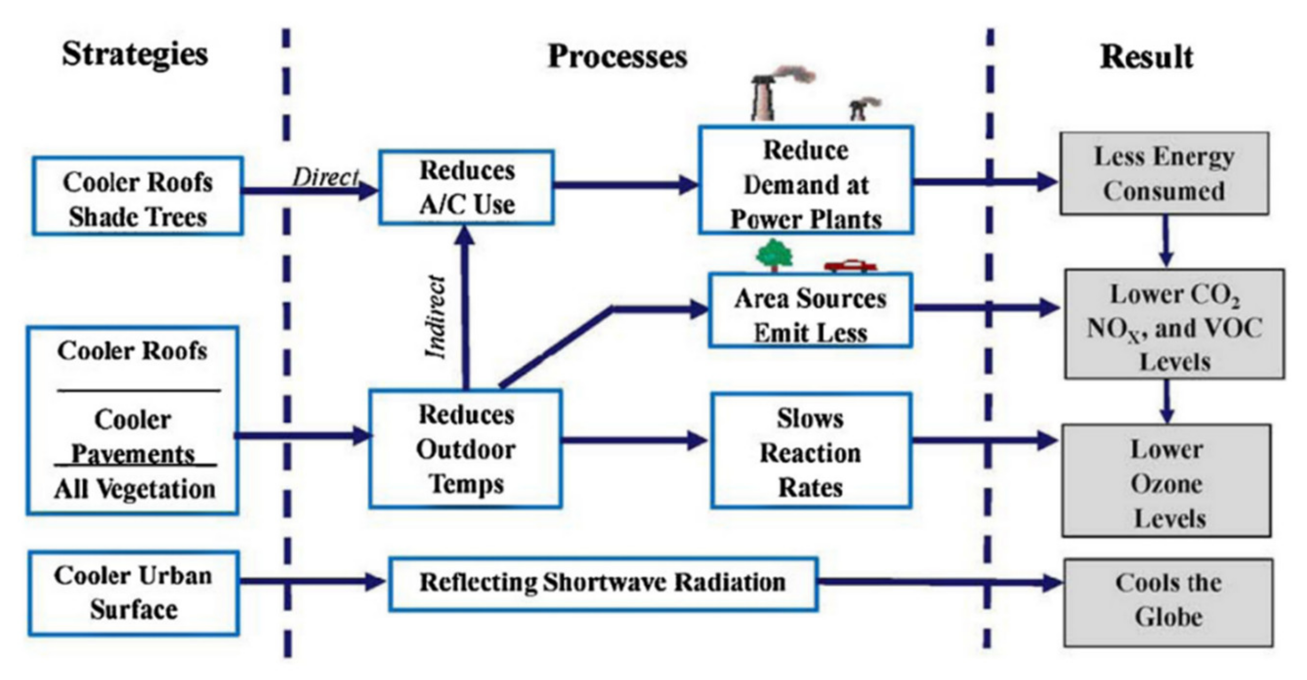Figure 1 shows the effects of heat island countermeasures.

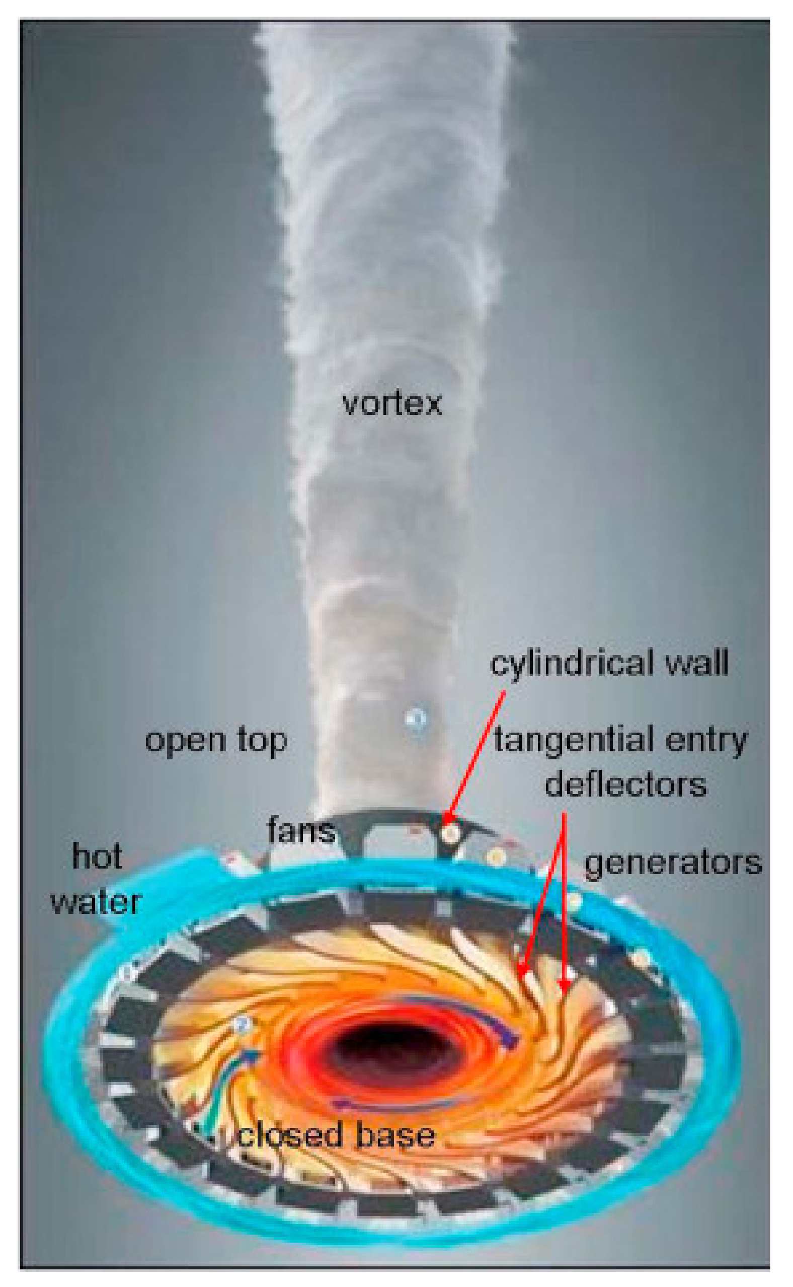
Within the artificial methods, this work aims to break the UHI effect using an atmospheric vortex engine (AVE) as a UHI-mitigation technology. The AVE is a device that was developed to generate mechanical energy employing a controlled tornado-like vortex [24]. The vortex is produced by admitting air tangentially at the base of a circular wall, which creates a convective vortex that acts as a chimney. The vortex is started by temporarily heating the air near the station’s center with fuel or steam. An AVE operates on these facts; the atmosphere is heated from the bottom and cooled from the top, and the expansion of heated gas produces mechanical energy. This principle is used to extract heat from the lower levels to the upper atmosphere to reduce the UHI effect. The schema of AVE is shown in Figure 2.

The research on AVEs as environmental control applications is not fully developed and presents an opportunity for present and future works. Numerous experimental and numerical studies have been carried out to investigate the main physical phenomena involved in convective vortex systems. Dessens [26,27] proposed an artificial tornado using the theory of convection eddies, demonstrating the theoretical possibility of using convective vortices. Michaud (1975) developed the design of a device capable of producing a convective vortex (small-scale tornado) through which horizontally mounted turbines could generate electricity [28]. Improving with his research, Michaud (1995) analyzed the specific process during the convection of the heat increase from the thermodynamic point of view [24,29,30]. Later, Michaud (2000) compared the convection process of atmospheric rising heat with the Brayton gas turbine cycle [31]. Finally, Michaud (2001) calculated the hurricane intensity using the total energy equation method [32]. In general, Michaud contributed enormously to investigating the concepts that deal with convective vortex systems because he was the first researcher that proposed a possible technical use of convective vortices as heat engines. The research in recent years has focused on CFD analysis of a convective vortex system model-scale [33,34,35,36,37]. The results have indicated that the engine can generate a vortex flow in the atmosphere much above its dimensions, then the vortex acts as a physical chimney, i.e., it isolates the hot air cloud from the surrounding air. Surprisingly, no study has been conducted that establishes a new concept in using convective vortex systems to mitigate urban heat islands.

Hidalgo developed an exergy theory to determine the main features of the vortex engine for cooling tower chimney, such as efficient use of energy and structure’s height [38]. Wang introduced the vertical convective urban vortex engine system (Figure 3) in a reduced-scale model to find out the system’s ability to strengthen the vertical convection and speed up the atmospheric circulation weakening the urban heat island effects [39].

The proposed concept called the urban vortex engine system (UVES consists of a vortex engine coupled to the bottom of high-rise buildings in the financial district center. This configuration resembles the interior of the buildings to a chimney that will guide the acceleration of urban warm air convection and accelerate the diffusion of pollutants, thus reducing the effect of Urban Heat Island.

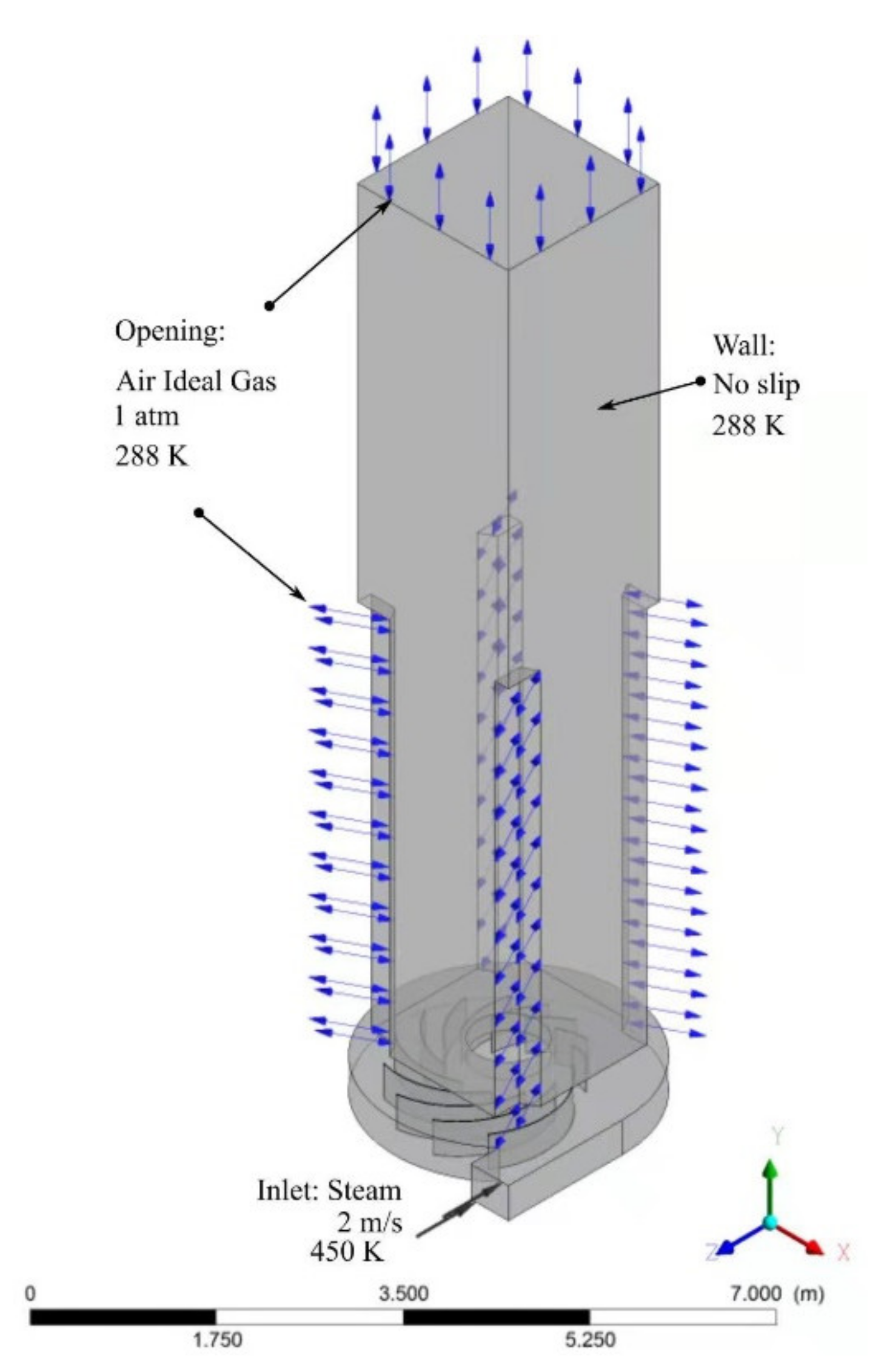
This work studies an atmospheric vortex engine coupled to a direct-contact cooling tower. The coupling of a cooling tower will improve vertical convection, increase the stability of the vortex, and improve efficiency by adding steam-air to the system. A multicomponent (steam-air) simulation is carried out in Ansys 19 to verify the device’s viability. The experimental section takes measures of pressure, velocity, and temperature to evaluate the system’s behavior. In the structural component (buildings), the fluid leaks and errors in heat transfer will be eliminated, isolating the system. Finding the optimal distance between each building is of interest for an actual application.

2. Physical Model and Numerical Methodology

2.1. Governing Equations

The primary laws required for computational fluid dynamics are the three equations of the flow control: continuity equation, momentum equations, and the energy conservation equation [40].

2.1.1. Continuity Equation

$$\frac{\partial \left(\rho \right)}{\partial t}+\nabla \cdot \left(\rho U\right) =0$$

(1)

where $\rho$ is the density of the fluid, $U$ is the vector of velocity, $\nabla$ is the vector operator, and $t$ is time.

2.1.2. Momentum Equation

$$\frac{\partial \left(\rho U\right)}{\partial t}+\nabla \cdot \left(\rho U\otimes U\right)=-\nabla \cdot \tau +S_M$$

(2)

where $\tau$ is the stress tensor, and $S_M$ is the momentum source. By utilizing specific tensor notation, the equations relating to each dimension can be combined into a single equation, and the stress tensor $\tau$ is related to the strain rate by the Equation (3).

$$\tau =\mu \left(\nabla U+{\left(\nabla U\right)}^T-\frac{2}{3}\delta \nabla \cdot U\right)$$

(3)

where $\delta$ is the identity matrix or Kronecker delta function, and $\mu$ is the dynamic viscosity.

2.1.3. Energy Conservation Equation

The energy conservation equation describes the internal temperature distribution of a system—the three-dimensional, non-steady-state equation in a rectangular coordinate system in Equation (4).

$$\frac{\partial \left(\rho T\right)}{\partial t}+\frac{\partial \left(\rho U_{x}T\right)}{\partial x}+\frac{\partial \left(\rho U_{y}T\right)}{\partial y}+\frac{\partial \left(\rho U_{z}T\right)}{\partial z}=\frac{\partial }{\partial x}\left(\frac{K}{C_p}\frac{\partial T}{\partial x}\right)+\frac{\partial }{\partial y}\left(\frac{K}{C_p}\frac{\partial T}{\partial y}\right)+\frac{\partial }{\partial z}\left(\frac{K}{C_p}\frac{\partial T}{\partial z}\right)$$

(4)

where $C_p$ is the specific heat capacity at constant pressure, $T$ is the temperature of the fluid, $K$ is the thermal conductivity of the fluid, and ($x, y, z$) are the axes of the coordinate system.

2.1.4. Turbulence Model

The k-epsilon model assumes the turbulence viscosity is connected to the turbulence kinetic energy [41,42] and dissipation via the Equation (6).

$${\mu }_t=C_{\mu }\rho \frac{k^2}{\epsilon }$$

(5)

where, ${\mu }_t$ is the turbulent viscosity, $C_{\mu }$ is a k-ε turbulence model constant (0.09), k is the turbulence kinetic energy per unit mass ($m^2/s^2$), and $\epsilon$ is the turbulence dissipation rate ($m^2/s^3$). The values of k come directly from the differential transport equations for the turbulence kinetic energy and turbulence dissipation rate [43] shown in Equation (6).

$$\frac{\partial \left(\rho k\right)}{\partial t}+\frac{\partial }{\partial x_j}\left(\rho U_{j}k\right)=\frac{\partial }{\partial x_j}\left[\left(\mu +\frac{{\mu }_t}{{\sigma }_k}\right)\frac{\partial k}{\partial x_j}\right]+P_k-\rho \epsilon +P_{kb}$$

(6)

where: ${\sigma }_k$ is constant (1.0), $P_{kb}$ is the turbulence production, and $P_k$ is the shear production of turbulence.

The RNG k-epsilon model is established on the renormalization group analysis from Navier–Stokes’s equations [44,45]. The transport equations for turbulence generation and dissipation are the same as those for the standard k-epsilon model. However, the model constants are different. The function $C_{\epsilon 1RNG}$ replaces the constant $C_{\epsilon 1}$.

The transport equation for turbulence dissipation is shown in Equation (7).

$$\frac{\partial \left(\rho \epsilon \right)}{\partial t}+\frac{\partial }{\partial x_j}\left(\rho U_j\epsilon \right)=\frac{\partial }{\partial x_j}\left[\left(\mu +\frac{{\mu }_t}{{\sigma }_{\epsilon RNG}}\right)\frac{\partial \epsilon }{\partial x_j}\right]+\frac{\epsilon }{k}\left(C_{\epsilon 1RNG}{P}_k-C_{\epsilon 2RNG}\rho \epsilon +C_{\epsilon 1RNG}{P}_{\epsilon b}\right)$$

(7)

where,

$$C_{\epsilon 1RNG}=1.42-f_{\eta }$$

(8)

$$f_{\eta }=\frac{\eta \left(1-\frac{\eta }{4.38}\right)}{\left(1+{\beta }_{RNG}{\eta }^3\right)}$$

(9)

$$\eta =\sqrt{\frac{P_k}{\rho C_{\mu RNG}\epsilon }}$$

(10)

where $\left(\begin{array}{cc}\begin{array}{ccc}{\sigma }_{\epsilon RNG}& C_{\epsilon 1RNG}& C_{\epsilon 2RNG}\end{array}& C_{\mu RNG}\end{array}\right) = \left(\begin{array}{cccc}0.7179& 1.68& 0.09& 1.0\end{array}\right)$ are RNG k–ε turbulence model constants, and $f_{\eta }$ is an RNG k-ε turbulence model coefficient.

The RNG k–ε turbulent model was selected to solve the complex turbulent flow modeling in the study of natural convection vortices. Ozalp and JayaKrishna used the RNG turbulence model to numerically analyze the internal flow field of a solar-heated vortex generator [46]. Natarajan verified that the RNG model successfully simulates the turbulent flow field in the vortex engine [33]. Chen reported that the RNG k–ε model is more suitable than the standard k–ε model to the rapidly strained and great curving streamline flows [47].

The advantages of using this approach were that the RNG turbulent model explains the effect of the swirl on the turbulence, thus improving the accuracy of the swirling flows [48]. RNG provides an analytical formula for the turbulent number of Prandtl compared to the k–ε turbulent model, which uses a constant value.

2.2. Computational Model and Boundary Conditions

The discretization of the control volume was carried out with ANSYS Meshing. Moreover, the concept of orthogonal quality evaluated the quality of the mesh. The range for orthogonal quality is 0–1, where a value of 0 is the worst, and a value of 1 is the best. For the resulting final mesh, the maximum orthogonal quality recorded was 1, the minimum was 0.54, and the average quality was 0.97. Based on these data, it is concluded that the result of the mesh captures all the essential details of the geometry and facilitates a better convergence. Figure 4 and

Table 1. Meshing methodology.

Meshing Procedure	Feature	Description
General mesh controls	Size function	Curvature
	Max face size	60 mm
	Inflation	First layer thickness
	First layer height	10 mm
	Maximum layers	5
Mesh method	Method	Multizone
	Mapped mesh type	Hexa/Prism-structured mesh
	Minimum edge length	10 mm
Local mesh controls	Face sizing	Name selections: inlet and opening 1
	Element size	20 mm
	Size function	Uniform

summarize the meshing methodology followed in the UVS flow simulation.

2.3. Boundary Conditions

The boundary conditions and pre-set were carried out with the third cell of the fluid flow CFX analysis, which is the ANSYS Setup. ANSYS set up cell works with CFX Pre-processor, where flow physics, boundary conditions, initial values, and solver parameters are specified.

Firstly, the pre-set process established a stationary single domain and a steady-state analysis, which means the flow characteristics do not change over time. The atmospheric pressure and buoyancy values were set at 1 atm and 9.81 $\mathrm{m}/{\mathrm{s}}^2$ (Y-axis direction), respectively.

In this study, the material investigated was a Wet Steam 3vl, IAPWS IF97 (273 K–550 K, 0.100 KPa–200 KPa) [49]. The advantage of using wet steam 3vl was that it was possible to simulate two fluids. A first fluid corresponds to a mixture of a variable composition containing the materials Steam3v (dry steam) and Air Ideal Gas. Moreover, a second fluid corresponds to a fixed composition mixture containing only the Steam3l material (liquid water). In a mixture of variable compositions, the proportion of each component material will change throughout the simulation. In contrast, in a mixture of fixed compositions, the proportion of each component material is fixed.

Due to the vortex effect in the center of the domain, it is not correct to configure the outlet boundary condition with a constant value. The output of the vortex stability zone was extended to avoid convergence problems. The extension was twice the width of the vortex stability zone, and the boundary condition was changed to “opening”. This change created a buffer between the output and the environment, which led to the convergence of numerical simulation calculations.

The final boundary conditions are:

• Vortex generator inlet: normal speed 2 m/s, static temperature 450 K; mass fraction: gas mixture {1}, liquid {0}. Set to an inlet boundary condition.
• Vortex stability zone inlet: relative pressure 0 Pa, opening temperature 288 K; mass fraction: air ideal gas {1}, steam 3v {0}. Set to opening boundary condition.
• Vortex stability zone outlet: relative pressure 0 Pa, opening temperature 288 K; mass fraction: air ideal gas {1}, steam 3v {0}. Set to opening boundary condition.
• UVS wall surface: temperature 15 °C. Set to wall boundary condition. The flow direction of the numerical model is shown in Figure 5.

2.4. Sensitive Study for the Simulation Case

The concept of orthogonal quality evaluated the quality of the mesh. The range for orthogonal quality is 0–1, where a value of 0 is the worst, and a value of 1 is the best. For the resulting final mesh, the maximum orthogonal quality recorded was 1, the minimum was 0.54, and the average quality was 0.97. Based on these data, it is concluded that the final result of the mesh captures all the essential details of the geometry and facilitates a better convergence [50].

The number of elements of the numerical simulation model of the urban vortex system was approximately 800,000. When the number of grids is around 400,000, 500,000, 800,000, and 1.5 million, the velocity of the gas mixture (steam) in the radial line in the vortex stability zone was selected as y = 2 m, as shown in Figure 6, and when the mesh has a low number of elements (less than 800,000), the values in the steam velocity vary significantly. In contrast, when the number of elements in the mesh is more significant than 800,000, the values in the vapor velocity stabilize, registering an average standard deviation of 0.0266.

3. Experimental Validation

This section aims to use the vortex engine principle to establish a layout of the building capable of forming vortices spontaneously under the action of natural vertical convection. First, an industrial gas burner coupled to a water heating system is used to heat the internal air to generate an internal and external temperature difference; thus, the hot air flows upwards. At the same time, it is possible to generate a tangential flow through the guide vanes to form a vortex, which is fundamentally different from the artificial method.

3.1. Urban Vortex System (UVS)

The urban vortex system (UVS) that simulates the layout of the buildings in an actual city is 5-m high. The test bench where the vortex is created to evaluate its stability and strength consists of the following components: metallic structure, which represents urban buildings; vortex generator; steam generator system; and measurement equipment. Figure 7 shows the schematic diagram of the UVS.

A set of triangular-shaped metal structures forms the vortex stability zone to simulate urban buildings on a scale of 1:40. The vortex generator has an atmospheric vortex engine, a cement base, a fluid inlet, and thermal insulation layers.

3.1.1. Vortex Generator

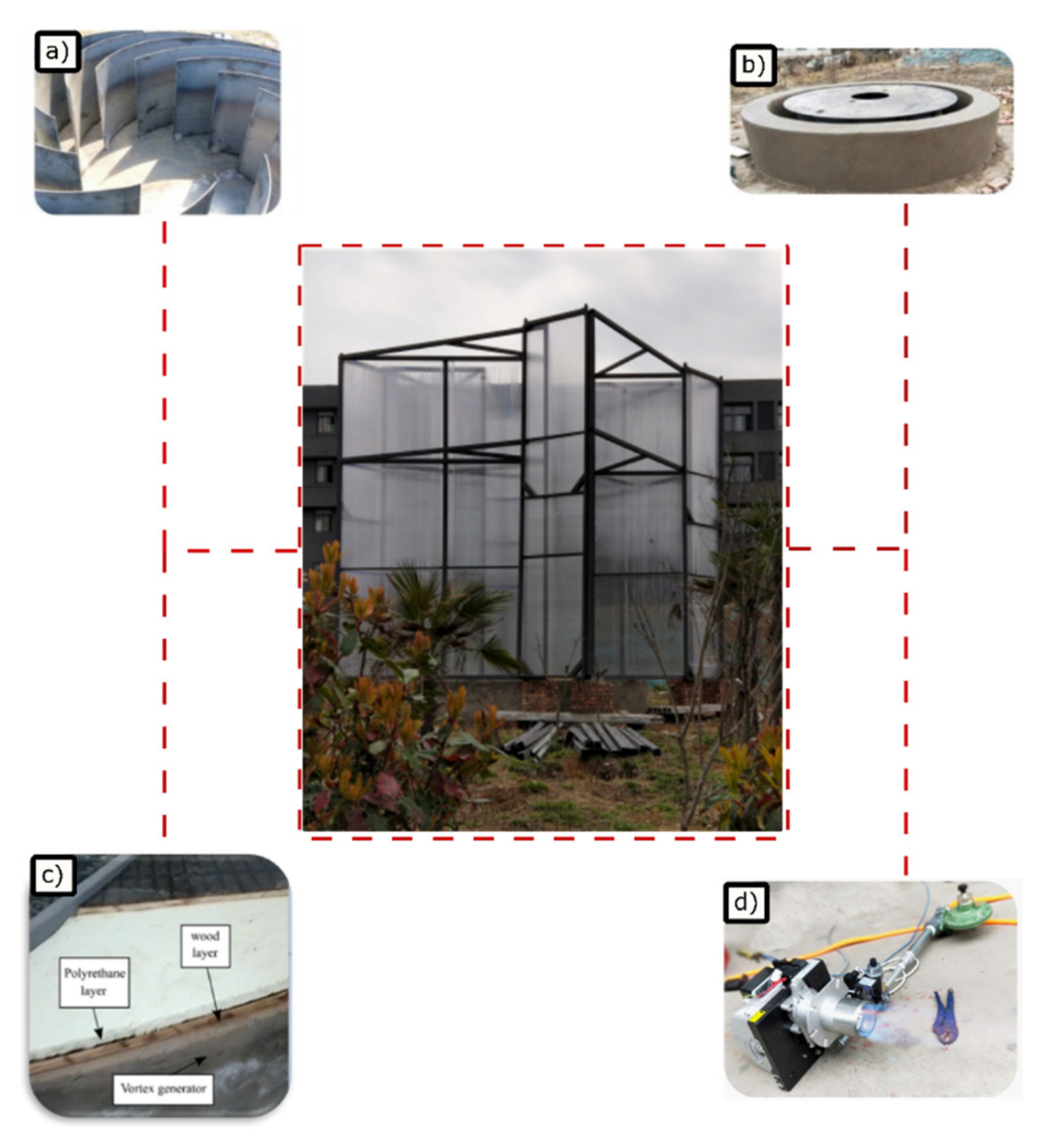
The vortex generator has an atmospheric vortex engine, a cement base, a fluid inlet, and thermal insulation layers. The atmospheric vortex engine is mainly composed of two round, steel plates with 10-mm thickness and 3000-mm diameter. The distance between the top and bottom plates is 760 mm. There are 12 thin-walled blades between the two round steel plates. The shape of the vanes is used to guide the flow of steam in the tangential direction (Figure 8a). The base supports the weight of the metal structure and forms, with the atmospheric vortex engine, a volume of warm air and steam supplies. The materials used were brick and concrete, which also serve as a thermal insulator. Its general dimensions were: 4 m outside diameter, 3.5 m bottom diameter, and 0.8 m height (Figure 8b). Finally, the fluid inlet is a rectangular opening in the tangential direction of the base. Its dimensions are: 0.4 m width, 0.5 m length, and 1 m height. Two layers of wood and polyurethane thickness of 1 cm each are adhered at the top of the base using spray foam polyurethane to reduce heat transfer with the outside environment and conserve the heat inside the vortex generator (Figure 8c).

3.1.2. Steam Generator System

The steam generator system was mounted in front of the fluid inlet. This system was divided into two groups: the gas burner set and the water sprayer dispenser. The air inside the vortex generator was heated using a Riello gas burner, a gas train multiblock, a gas pressure gate, and an LPG gas cylinder. The main characteristics of each component are summarized in

Table 2. Main features of a gas burner set.

Component	Feature	Description
Gas burner	Model	40F5
	Thermal power	23–53 kW
	Gas type	Natural gas/LPG
	Pressure	Min. 10 mbar–max. 40 mbar
Gas train multiblock	Model	MB 4005/1
	Gas type	Natural gas/LPG
	Connection train-burner	Rp 1/2
Gas pressure gate	Outlet pressure ranges	20.7 KPa to 690 KPa
	Connection	NPT 1/2
LPG gas cylinder	Size	45–50 kg

. It is important to note that the air pressure switch on the gas train multiblock was regulated to 0.09 KPa for the correct performance of the gas burner.

The supplies steam is generated by entering water spray into the vortex generator. The gas burner heats the indoor air to a temperature above 100 °C to evaporate the water entering the dispenser. The equipment used to spray the water was a Yijin electric double-pump dispenser.

Table 3. Features of electric sprayer dispenser.

Component	Feature	Description
Electric sprayer	Type	Double pump
	Capacity	20 L
	Power	12–20HA Lithium battery
	Weight	5 kg
	Dimensions	38 × 20 × 40 cm

provides the main features of the dispenser.

3.1.3. Temperature and Velocity Measurement Equipment

The steam and hot air vortex created in the center of the vortex stability zone have high rotational velocities at its center, so multiple temperature measurement points must be arranged. The temperature field in the experiment was measured with a thermocouple. For the vortex generator inlet and the vortex stability measurements, thermocouples type K were fixed at the corresponding points and connected to the CENTER309 four channels’ data logger thermometer, as shown in Figure 9.

The experiment uses the KIMO AMI300 multifunctional measuring instrument to measure velocity. The instrument is shown in Figure 10. Wind speed is measured using a sensitive direct-line measurement. The measurement range is 0.05–3 m/s with a resolution of 0.01 m/s. The end of the speed measurement can be extended and retracted within 1 m.

3.2. Experimental Setup and Procedure

Several points were established within the vortex generator (V.G.) and vortex stability zone (VSZ) to capture the experimental variables. The main variables were temperature and velocity. The temperature measurement points were mainly in two locations, the V.G. and the VSZ, using horizontal and vertical lines, as detailed in Figure 11. For the measurement process, eight control lines, seven horizontal and one vertical, were established. The horizontal lines have four measurement points; on the contrary, the vertical line has eight measurement points. The first control line, L1, was located at the entrance of the V.G.; the steam temperature measurements were taken at a depth of 0.2 m at the middle of vortex generator height. In addition, this line recorded the temperature value when entering the last thin-walled blade. The L2 control line is a vertical line with eight measurement points that starts at the center of the V.G. and ends at the height of 2 m inside the VSZ.

All measurements in the vortex stability zone were made in the airflow center at different heights: L3, h = 0 m; L4, h = 0.4 m; L5, h = 0.8 m; L6, h = 1.2 m; L7, h = 1.6 m; and L8, h = 2.0 m, respectively; in total, there are six horizontal lines with 24 measurement points.

The experimental test was a steady-state process. Thus, the system must be heated first and then measured after all parameters are stable (

Table 4. Experimental process.

Step	Task
1	Check the operation of each measuring instrument, then open the gas valve gradually to guarantee a stable convection zone.
2	Turn on the gas burner and insert a K-type thermocouple at a depth of 20 cm at the entrance of the V.G. to record the temperature. When the air temperature reaches 450 K, the water sprayer is activated.
3	Record the temperature and velocity measurements, establishing a short time between them in which the vortex generated is stabilized.
4	Change the entrance width of the vortex stabilization chamber for the next set of data measurements.
5	Repeat the experiment several times. After eliminating the deviation value, take the average value of each group of data as an experimental result.

).

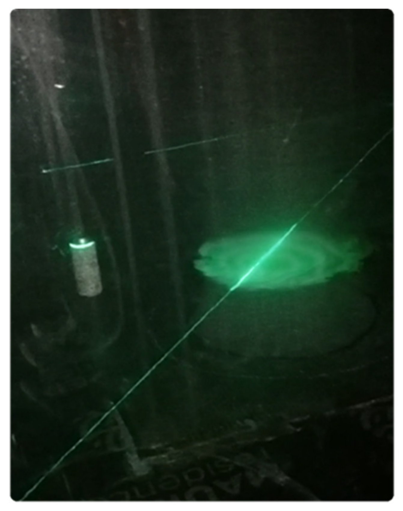
The steam generated at the entrance of the V.G. is expelled towards the VSZ with intense vorticity, as shown in Figure 12. A green pedestal laser was used for better visualization of the phenomenon

The temperature in the vortex core will be significantly higher than the ambient temperature. The velocity field will also keep the velocity in the vortex core higher than the surrounding velocity. The tangential velocity of the external flow field is more significant than zero; therefore, the temperature field of the flow field is measured. Figure 13 shows the location of the temperature measurement points on the UVS model.

3.3. Dimensional Analysis

In this section, repeating variables to generate non-dimensional parameters are used in the urban vortex system. The primary phenomenon is natural convection because the warm mixture enters the center of the vortex generator through twelve tangential blades that produce a convective vortex. Figure 14 shows the dimensional variables, the non-dimensional variables, and the dimensional constants into the UVS.

The procedure for obtaining the dimensionless parameters existing in the UVS is detailed below.

Step 1: $f^{\prime }=\left(F_{out},\rho ,\mu ,k,C_p,L,\mathsf{\Delta }T\beta g,V\right)$, so N° of variables, $n=8$.

Step 2: $F_{out}=\left[\frac{ML}{T^2}\right]$, $\rho =\left[\frac{M}{L^3}\right]$, $\mu =\left[\frac{M}{LT}\right]$, $k=\left[\frac{ML}{T^3\theta }\right]$, $C_p=\left[\frac{L^2}{T^2\theta }\right]$, $L=\left[L\right]$, $\Delta T=\left[\theta \right]$, $\beta =\left[{\theta }^{-1}\right]$, $g=\left[\frac{L}{T^2}\right]$, $V=\left[\frac{L}{T}\right]$. N° of fundamental dimensions ($M$, $L$, $T$, $\theta$) involved $m=4$.

Step 3: The 4 variables $L,\mathsf{\Delta }T,\beta ,\mathrm{and} g$ cannot be formed into a dimensionless group, so the reduction number $k=4$.

Step 4: N° of dimensionless Π groups needed = n – k = 8–4 = 4... $\therefore \hspace{0.33em}f\left({\mathsf{\Pi }}_1,{\mathsf{\Pi }}_2,{\mathsf{\Pi }}_3,{\mathsf{\Pi }}_4\right)=0$.

Steps 5 and 6: Select the following $k=4$ variables to be primary (repeating): $F_{out},\rho ,\mu ,k,C_p$.

The dimensionless parameters existing in the UVS are detailed in Equations (11)–(15).

$$\begin{array}{c}For\hspace{1em}{\Pi }_1={\mu }^a{k}^b{\rho }^c{V}^d{F}_{out}:\hspace{1em}{M}^0{L}^0{T}^0{\theta }^0={\left(\frac{M}{LT}\right)}^a{\left(\frac{ML}{T^3\theta }\right)}^b{\left(\frac{M}{L^3}\right)}^c{\left(\frac{L}{T}\right)}^d\left(\frac{ML}{T^2}\right)\hfill \\ M:\hspace{1em}0=a+b+c+1;\hspace{1em}L:\hspace{1em}0=-a+b-3c+d+1;\hspace{1em}\hfill \\ T:\hspace{1em}0=-a-3b-d-2;\hspace{0.33em}\hspace{1em}\theta :\hspace{1em}0=-b;\hfill \\ Solving:\hspace{1em}a=-2;\hspace{0.33em}b=0;\hspace{0.33em}c=1;\hspace{0.33em}d=0.\hspace{1em}Then\hfill \\ \hspace{1em}\hspace{1em}\hspace{1em}\hspace{1em}\hspace{1em}\hspace{1em}\hspace{1em}\hspace{1em}{\mathsf{\Pi }}_1={\mu }^{-2}{k}^0{\rho }^1{V}^0{F}_{out}=\boxed{F_{out}\rho /{\mu }^2}\hfill \end{array}$$

(11)

$$\begin{array}{c}For\hspace{1em}{\Pi }_2={\mu }^a{k}^b{\rho }^c{V}^d{C}_p:\hspace{1em}{M}^0{L}^0{T}^0{\theta }^0={\left(\frac{M}{LT}\right)}^a{\left(\frac{ML}{T^3\theta }\right)}^b{\left(\frac{M}{L^3}\right)}^c{\left(\frac{L}{T}\right)}^d\left(\frac{L^2}{T^2\theta }\right)\hfill \\ M:\hspace{1em}0=a+b+c;\hspace{1em}L:\hspace{1em}0=-a+b-3c+d+2;\hspace{1em}\hfill \\ T:\hspace{1em}0=-a-3b-d-2;\hspace{0.33em}\hspace{1em}\theta :\hspace{1em}0=-b-1;\hfill \\ Solving:\hspace{1em}a=1;\hspace{0.33em}b=-1;\hspace{0.33em}c=0;\hspace{0.33em}d=0.\hspace{1em}Then\hfill \\ \hspace{1em}\hspace{1em}\hspace{1em}\hspace{1em}\hspace{1em}\hspace{1em}\hspace{1em}\hspace{1em}{\mathsf{\Pi }}_2={\mu }^1{k}^{-1}{\rho }^0{V}^0{C}_p=\mu C_p/k=\boxed{Pr}\hfill \end{array}$$

(12)

$$\begin{array}{c}For\hspace{1em}{\Pi }_3={\mu }^a{k}^b{\rho }^c{V}^{d}L:\hspace{1em}{M}^0{L}^0{T}^0{\theta }^0={\left(\frac{M}{LT}\right)}^a{\left(\frac{ML}{T^3\theta }\right)}^b{\left(\frac{M}{L^3}\right)}^c{\left(\frac{L}{T}\right)}^d\left(L\right)\hfill \\ M:\hspace{1em}0=a+b+c;\hspace{1em}L:\hspace{1em}0=-a+b-3c+d+1;\hspace{1em}\hfill \\ T:\hspace{1em}0=-a-3b-d;\hspace{0.33em}\hspace{1em}\theta :\hspace{1em}0=-b;\hfill \\ Solving:\hspace{1em}a=-1;\hspace{0.33em}b=0;\hspace{0.33em}c=1;\hspace{0.33em}d=1.\hspace{1em}Then\hfill \\ \hspace{1em}\hspace{1em}\hspace{1em}\hspace{1em}\hspace{1em}\hspace{1em}\hspace{1em}\hspace{1em}{\mathsf{\Pi }}_3={\mu }^{-1}{k}^0{\rho }^1{V}^{1}L=V\rho L/\mu =\boxed{Re}\hfill \end{array}$$

(13)

$$\begin{array}{c}For\hspace{1em}{\Pi }_4={\mu }^a{k}^b{\rho }^c{V}^d\left(\mathsf{\Delta }T\beta g\right):\hspace{1em}{M}^0{L}^0{T}^0{\theta }^0={\left(\frac{M}{LT}\right)}^a{\left(\frac{ML}{T^3\theta }\right)}^b{\left(\frac{M}{L^3}\right)}^c{\left(\frac{L}{T}\right)}^d\left(\frac{L\theta }{T^2\theta }\right)\hfill \\ M:\hspace{1em}0=a+b+c;\hspace{1em}L:\hspace{1em}0=-a+b-3c+d+1;\hspace{1em}\hfill \\ T:\hspace{1em}0=-a-3b-d-2;\hspace{0.33em}\hspace{1em}\theta :\hspace{1em}0=-b;\hfill \\ Solving:\hspace{1em}a=1;\hspace{0.33em}b=0;\hspace{0.33em}c=-1;\hspace{0.33em}d=-3.Then\hfill \\ \hspace{1em}\hspace{1em}\hspace{1em}\hspace{1em}\hspace{1em}\hspace{1em}\hspace{1em}{\mathsf{\Pi }}_4={\mu }^1{k}^0{\rho }^{-1}{V}^{-3}\left(\mathsf{\Delta }T\beta g\right)=\boxed{\mathsf{\Delta }T\beta g\mu /\rho V^3}\hfill \end{array}$$

(14)

$$\begin{array}{c}\therefore {\mathsf{\Pi }}_1=f\left({\mathsf{\Pi }}_2,{\mathsf{\Pi }}_3,{\mathsf{\Pi }}_4\right)\\ F_{out}\rho /{\mu }^2=f\left(Pr,Re,\mathsf{\Delta }T\beta g\mu /\rho V^3\right)\end{array}$$

(15)

where $F_{out}$ is a buoyancy force, $\rho$ is the fluid density, $\mu$ is the dynamic viscosity of the fluid, $Pr$ is the Prandtl number, $Re$ is the Reynolds number, $\mathsf{\Delta }T$ is the temperature interval, $\beta$ coefficient of volumetric expansion, and $V$ is the velocity of the fluid. Cengel noted, “to ensure complete similarity, the model and prototype must be geometrically similar, and all independent $\mathsf{\Pi }$ groups must much between model and prototype” [51]. Under these conditions, the dependent $\mathsf{\Pi }$ of the model is guaranteed also to equal the dependent $\mathsf{\Pi }$ of the prototype, as can be seen from (15).

4. Results and Discussion

This section analyzes the behavior of the temperature, velocity, and pressure field within a modified vortex engine system designed to extract heat from an urban canopy under the circulation of heat islands.

The simulated velocity, pressure, and temperature data are analyzed in Section 4.1, Section 4.2 and Section 4.3, respectively. Specifically, in Section 4.3 the simulated temperature values are validated with experimental data for each vertical and horizontal linear control line. In addition, the process of maximizing the output parameters in the simulation is carried out using Ansys CFX software’s advanced tool in Section 4.4. Finally, in Section 4.5 and Section 4.6, a thermodynamic and sustainability analysis is carried out, determining the UVS prototype’s thermal power and viability.

4.1. Effect of the Velocity Field

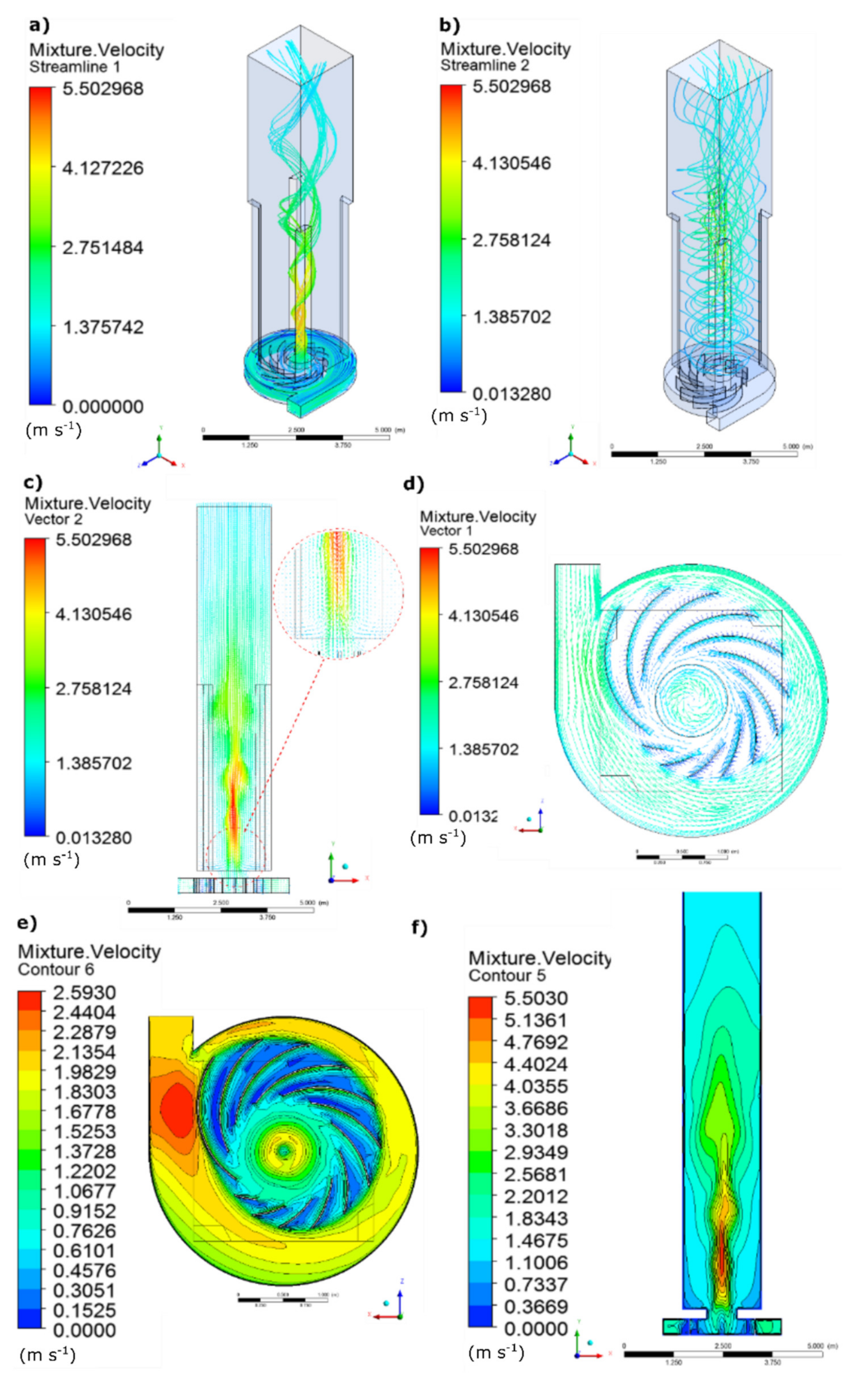
The streamlines of the vortex generator are shown in Figure 15a. The mixture steam-air initial velocity was 2 m/s and gradually increased. When converging at the center of the V.G., where the flow reaches a maximum of 2.48 m/s, vorticity was evident. From the radial direction, the axial velocity gradually increased from a low value to a maximum (natural vortex) and then gradually decreased. The peak value recorded was 4.707 m/s at 2.5 m height.

Similar behavior was observed in the streamlines of the VSZ. Under the action of the tornado vortex, the outside air entered from the inlet of the stability chamber, where the inlet velocity was approximately 0.352 m/s, continuously increasing to the maximum velocity at the outlet of 3.56 m/s, as indicated in Figure 15b.

Figure 15c,d show the results of velocity vectors; from these plots, it can be observed that the volume of the steam introduced was distributed uniformly through the twelve thin-walled blades; tangentially, it was directed until converged in the central area. Additionally, the direction of the fluid velocity at the inlet was horizontal, and when the fluid converged towards the center, it was vertical. The horizontal velocity component was almost zero in the central position, and the flow velocity gradually increased in the stability zone of the vortex.

The velocity field in the vortex generator is shown by the contour plot on the Z.X. plane, Y = −0.2 m, in Figure 15e. The velocity through the thin-walled blades was quantified at 1.52 m/s. The vapor entered tangentially into the V.G. nucleus, forming a stable vortex that started with an approximate velocity value of 0.61 m/s, it increased to a maximum value of 1.98 m/s, and then decayed to values of 1.68 m/s on the periphery.

Besides, the contour plot of the velocity magnitude in the plane XY is evaluated and shown in Figure 15f. The maximum velocity of 5.47 m/s was obtained at 2 m height. The figure shows that the rotation velocity gradually decreases from its center in the radial direction, which is consistent with the distribution of the natural vortex or is similar to a slightly distorted Rankine vortex.

The steam flow rotates at high velocity in the center of the stability chamber. However, as the height increases, the energy dissipates, and the velocity of the tangential flow outside gradually decreases. The maximum steam velocity recorded at the outlet of the vortex stability zone was 2.75 m/s, with outside air attracted towards the center at a rate of 0.80 m/s.

In addition, six horizontal lines located in the X.Z. plane of the model were analyzed. L1 and L2 were located at the height of 0.2 m and 0.5 m in the corresponding section of the vortex generator. It is important to note that L1 is located in the middle of the V.G. In contrast, L2 corresponds to the interface between V.G. and VSZ, whose diameter was 0.8 m.

On the other hand, the remaining four lines called L3, L4, L5, and L6 were in the vortex stability section with heights of 1.5 m, 2.5 m, 3.5 m, and 5.5 m, respectively. The last line L6 corresponded to the physical length of the experimental buildings.

Figure 16a shows the velocity values of the flow field located in the vortex generator. The chart presents a sinusoidal form due to the irregular geometry of the V.G. However, a similar pattern was identified in the range of X = −0.5; 0.5 m, where the stable vortex was formed. L1 has two peak values at the extreme points of the VG-VSZ interface. These values were 1.87 m/s and 1.96 m/s at the extreme points of the range of X= −0.15; 0.15 m. Afterward, symmetrically the velocity decreased to a value of 0.754 m/s in the central section of the model. Line L2 showed a behavior similar to L1, increasing the peak values of 18% and a velocity value of 1.70 m/s in the central section X = 0 m.

Finally, Figure 16b presents the velocity values of the flow field located in the vortex stability zone. It could be observed that the velocity values are maximum in the central section. The velocity gradient in the region X = −0.4; 0.4 m is greater in relation to other positions. All horizontal lines showed similar behavior; the maximum velocity value was 5.42 m/s located at h = 1.5 m. This velocity peak gradually decreased with a height to the value of 2.84 m/s at h = 5.5 m, which means a reduction of 47.6%.

4.2. Effect of the Pressure Field

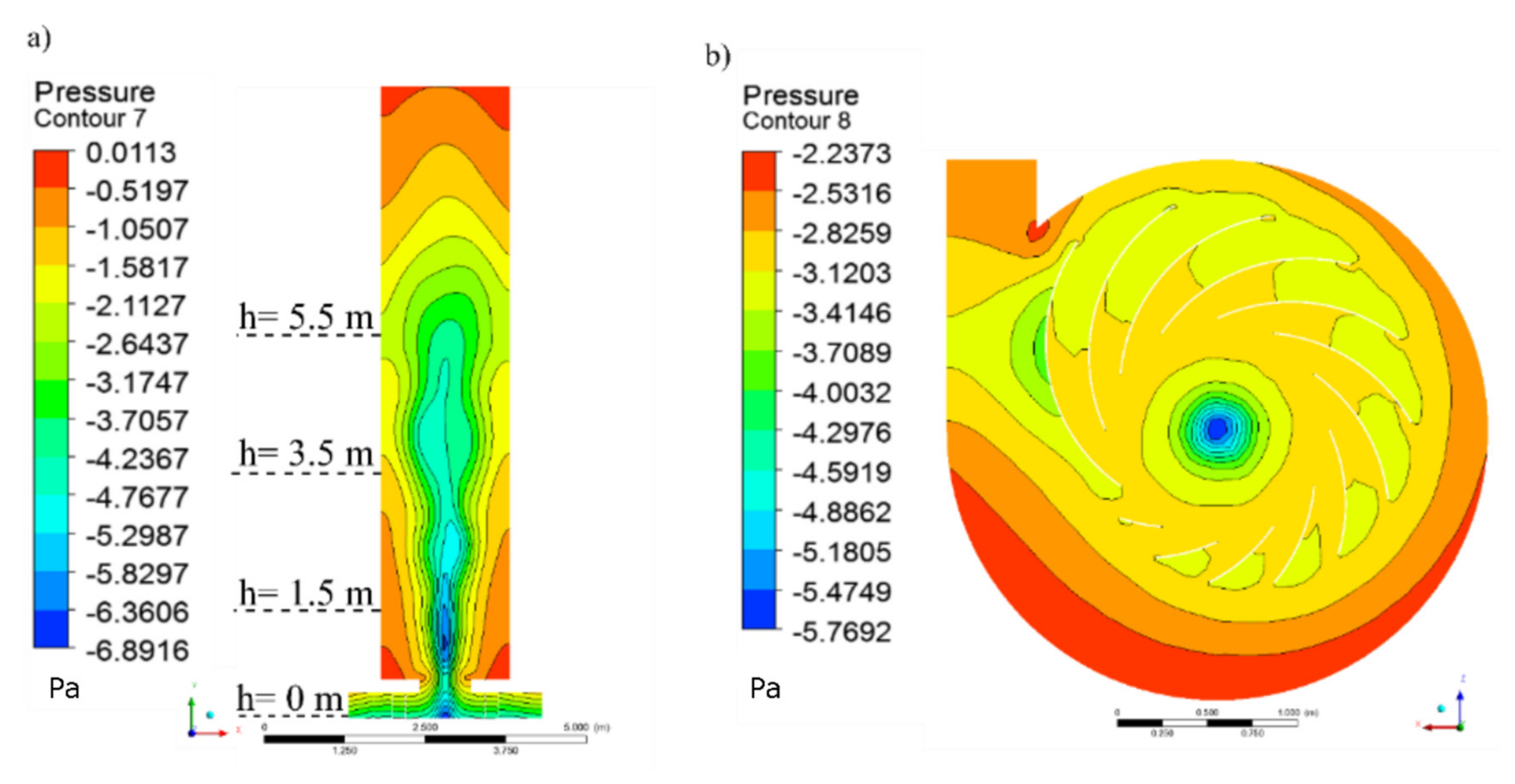
The pressure field of the vertical section of the flow field is displayed in Figure 17a. For the section of the vortex generator, a value of −6.89 Pa was obtained, and similarly for the section of vortex stability, the average value was −4.23 Pa. For the positions located at Y = 1.5 m; 3.5 m; 5.5 m, it could be observed that the recorded central pressure peak was −5.48 Pa; this value increased as a function of height to a value of −4.38 Pa at h = 5.5 m. Suction pressures to the center of the vortex were also recorded. The average value of the suction pressure at the entrance of the vortex stability zone was −0.992 Pa. This negative pressure caused the surrounding air and steam to be continuously absorbed. It is important to note that the negative central pressure decreased depending on the height of the UVS, with a minimum pressure value of 0.0113 Pa at 10 m. This value tends to 0 Pa, which represents the relative pressure set in the simulation.

The pressure field in the vortex generator is shown in the contour diagram in the X.Z. plane, Y = −0.2 m, as shown in Figure 17b. The pressure through the thin-walled blades was quantified at −2.83 Pa. The vapor entered tangentially into the V.G. nucleus, forming a stable vortex that started with an approximate pressure value of −5.77 Pa and increased to a maximum value of −3.41 Pa on the periphery.

4.3. Effect of the Temperature Field (Validation against Experimental Data)

This section presents the plots of the temperature contours on vertical plane X.Y. and horizontal plane X.Z.; the fitting procedure for each experimental measurement line applying mathematical modeling and the comparison between the simulated and experimental values for each horizontal vertical measurement line are thoroughly studied and well documented.

As seen in Figure 18a, the plot of the temperature contours on the vertical plane X.Y. is shown. It was observed that the initial temperature at the inlet of the model was 450 K and gradually decreased by the interaction with the twelve thin-walled blades at 288 K due to the heat-transfer mechanisms. The final steam temperature in the center of the vortex generator was 373–381 K. The coupling of a mixture vapor-air improves vertical convection, increases the stability of the vortex, and improves efficiency by adding steam-air to the system.

In the vortex stability zone, the temperature of the steam-air mixture was maintained around 353–364 K to an approximate height of 2.5 m above the vortex generator. This temperature gradually decreases with the height, becoming very similar to the ambient temperature in heights greater than 6 m. On the other hand, the plot of the temperature contours on the horizontal plane X.Y.; Y = 0.02 m is shown by Figure 18b. As shown from Figure 18b, the temperature field decreased about 60 K in the area of the thin-walled blades, reaching about 380 K in the central part of the vortex generator. It was also possible to appreciate that the formed vortex has about 0.4 m in diameter in the model.

The fitting analysis of the experimental results was carried out by using mathematical modeling, which allows us to find simple models such as polynomials equations. Therefore, it was first identified what type of adjustment corresponded to each measurement line. Then, it was calculated and represented the polynomial that best fits the collection of experimental data.

For measurement line L1, a linear fit was established for the existing data set. The variation of the temperature field present in the V.G. is a complex phenomenon; however, the linear adjustment was helpful to know how much the temperature decreases from the entrance to the last blade, as indicated in Figure 19. A quadratic fit was selected for the following L2 experimental data collection. The variation in temperature as a function of the height of the UVS model showed a gradual increase to a maximum point of 1 m. It then decreased to approximate values at ambient temperature (see Figure 19).

Similarly, the collection of experimental data from the L3 line (h = 0 m) in the VSZ were fitted using a quadratic fit. The temperature field is more significant in the vortex core and decreases symmetrically due to the horizontal distance. The summary of the curve fitting analyzes for lines L1, L2, and L3 are presented in

Table 5. Summary of the fitting analysis: Experimental L1 results.

Equation	Intercept		Slope		Statistics
y = a + b x	Value	Error	Value	Error	R-Square
	315.67	18.55	117.33	17.01	0.945

and

Table 6. Summary of the fitting analysis: Experimental L2 and L3 results.

Equation	Intercept		B1		B2		Statistics
y = Intercept + B1 x + B2 x2	Value	Error	Value	Error	Value	Error	R-Square
L2	379.14	2.10	33.27	4.96	−24.07	2.53	0.95
L3	401.81	2.68	5	5	−613.8	18.63	0.99

.

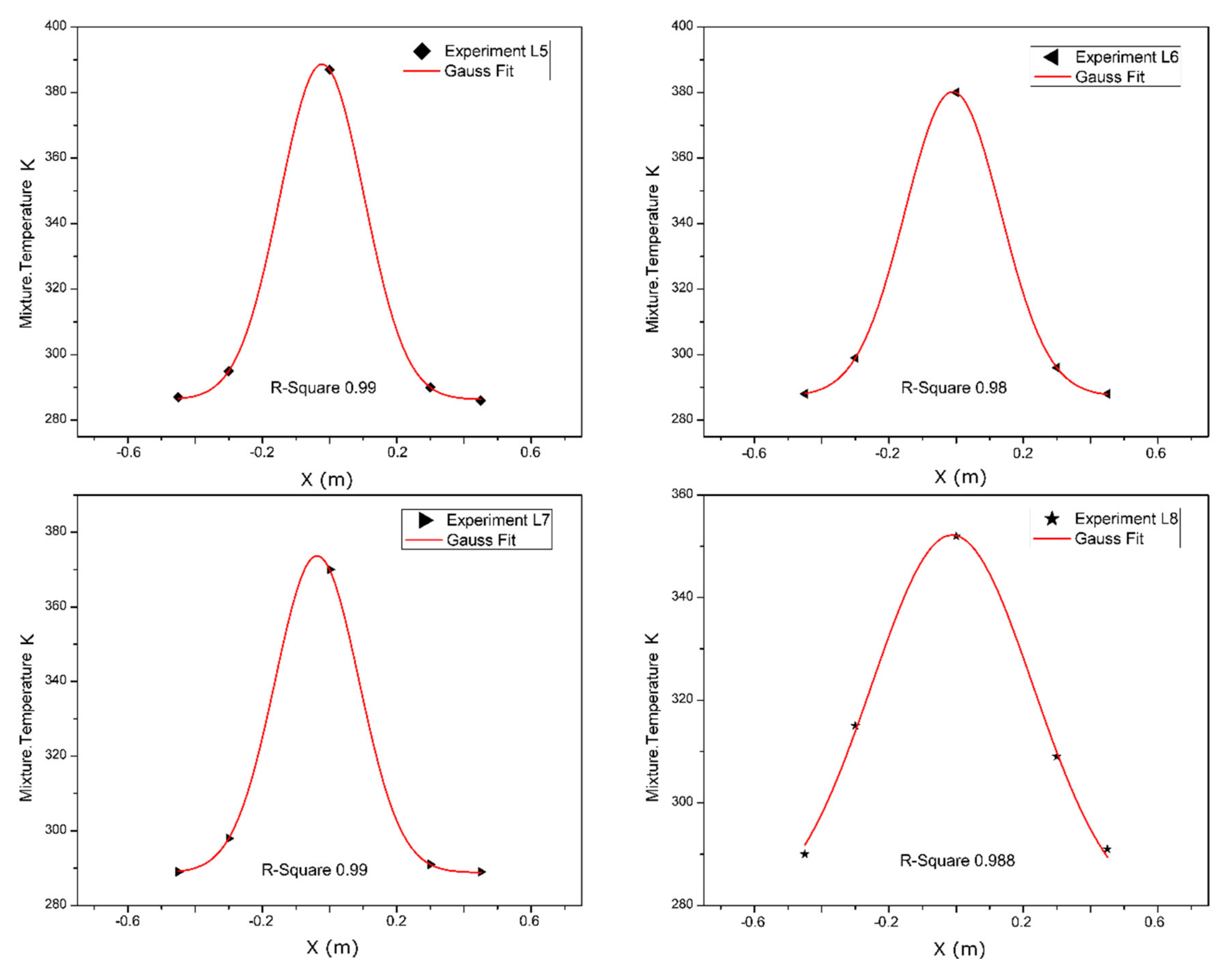
Furthermore, non-linear fit models were selected to fit the L4–L8 experimental measurement lines. The Gauss–Newton algorithm was employed to find the minimum global distance from all experimental points. Figure 19 and Figure 20 plot the Gauss fitting of the measurement lines from L4 to L8.

The Gaussian non-linear fit satisfactorily fitted the experimental data collection of the five horizontal lines. The analysis results calculated R-squared values close to unity with a standard deviation error of less than 10%, as can be seen from

Table 7. Summary of the fitting analysis: Experimental from L4 to L8 results.

Line	y0	xc	w	A	Statistics R-Square
L4	282.8 ± 6.5	−0.03	0.28	38.7 ± 8.3	0.97
L5	286.3 ± 0.4	−0.02	0.25	32.1 ± 0.7	0.99
L6	287.4 ± 0.2	−0.01	0.28	33.1 ± 0.2	0.99
L7	288.8 ± 0.2	−0.03	0.25	26.5 ± 0.2	0.99
L8	277.7 ± 7.0	−0.01	0.47	44.8 ± 8.4	0.98

.

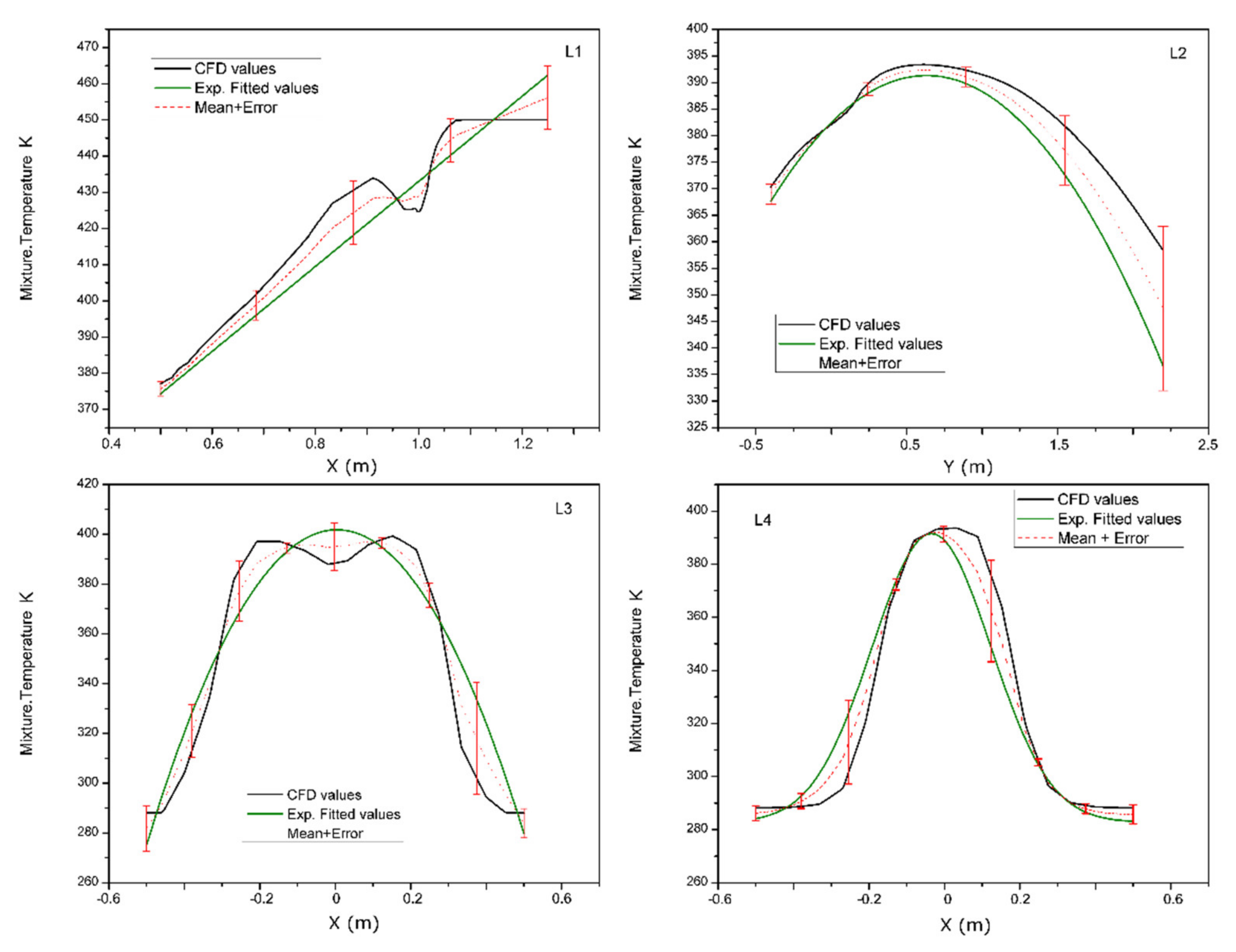
Finally, a comparison of the simulated and experimental temperature values of the horizontal and vertical measurement lines is shown in Figure 21 and Figure 22. It can be noticed that the global simulated value is in good agreement with the experimentally measured values; the simulating values are higher concerning the experimental data due to an actual process that always has irreversibility in the system.

The temperature field of the simulated and experimental data showed the same behavior. Temperature values were maximum in the nucleus of the vortex. However, they decreased symmetrically as a function of the horizontal distance and the height of the vortex.

Table 8. Standard deviation of the comparison between simulation and experiment values.

Measurement Line	Standard Deviation
L1	4.65%
L2	4.21%
L3	8.36%
L4	6.24%
L5	2.82%
L6	2.75%
L7	3.97%

shows the standard error deviation obtained from the comparison between simulated and experimental values in the measurement lines.

The previous comparative analysis shows that the numerical simulation is in good agreement with the experiment. The simulation deviation is approximately 6%. Therefore, this research concludes that numerical simulation can accurately simulate the internal flow field of the experimental test bench. In addition, numerical simulation can be used to optimize their structure.

4.4. Maximization of Y-Force and Speed Output Parameters

This section applied an advanced simulation tool available in the Ansys Workbench software called Design Xplorer. The Design Xplorer tool described the connection between design variables and the performance of the UVS simulation model using analysis of the design of experiments and response surfaces.

The velocity and temperature of the mixture (air ideal gas-vapor) at the vortex generator inlet were configured as input parameters. On the other hand, Out Velocity was the first output parameter, and it refers to the velocity of the gas mixture inside the UVS at the height of 10 m. In addition, a second output parameter called Out Force-Y was configured. It refers to the maximum force on the Y-axis exerted by the gas mixture at the UVS output (10 m height).

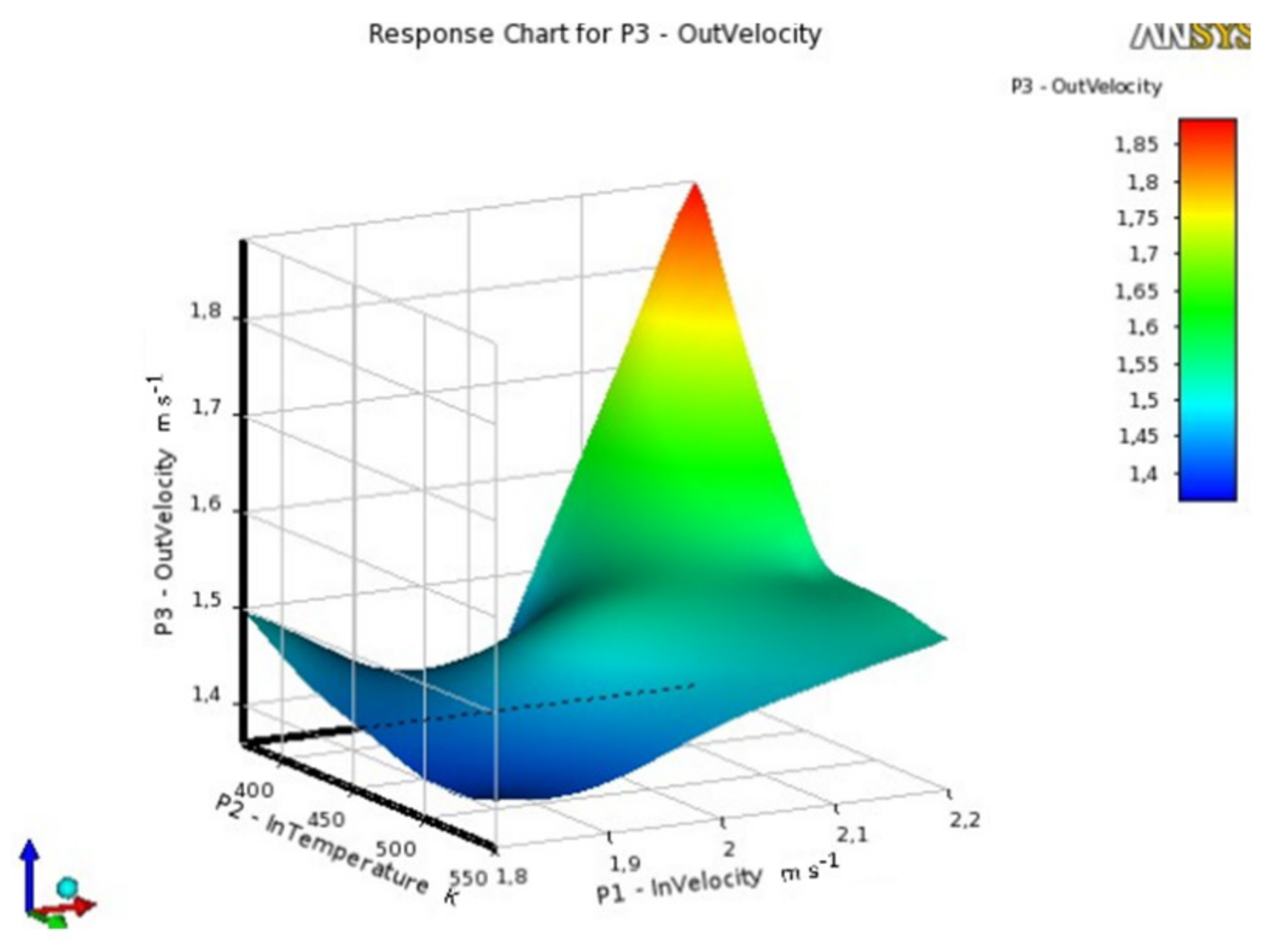
The results of the response surfaces showed the impact graphically that changing each input parameter has on the displayed output parameter. The Out-Velocity parameter varies proportionally with the input velocity; however, it is inversely proportional to the input temperature. Its peak value was 1.8841 m/s. This result was obtained with 2.2 m/s for the velocity input parameter and 373 K for the temperature input parameter, as detailed in Figure 23.

Similar behavior was observed for the other Out Force output parameter. This parameter varies linearly as a function of the input velocity of the steam mixture. Therefore, it presented a peak value of 6.3982 N for the value of 2.2 m/s. In contrast, the output force showed a parabolic variation as a function of the inlet temperature. Its peak value was 5.7241 N with an inlet temperature of 461.5 K, as can be seen in Figure 24.

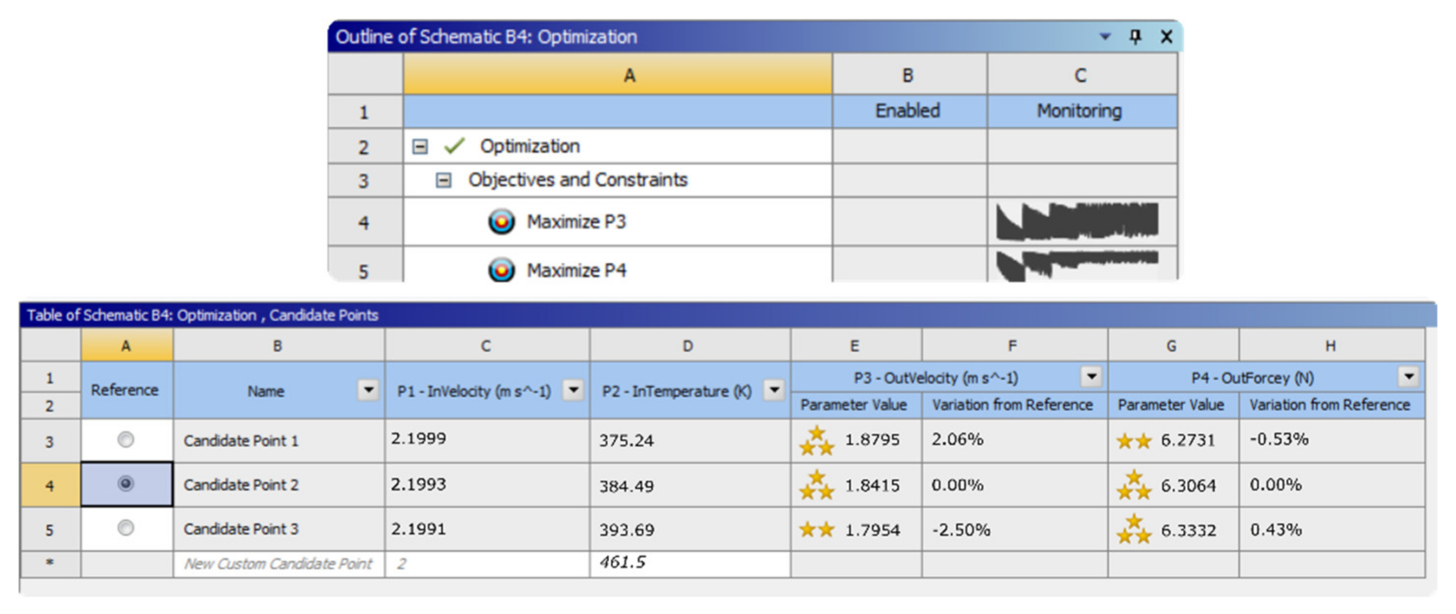
Finally, the optimization process of the UVS model was carried out by using the method of goal-driven optimization (GDO). The objective of the UVS model optimization process was to maximize the output parameters corresponding to the velocity and force outputs on the Y-axis as a function of the input parameters that represent the physical conditions of the vapor-air mixture when entering the vortex generator. Figure 25 reports that this method found a candidate point that obtained the best adjustment in the optimization, with a maximum value for the outlet velocity of 1.8415 m/s and a maximum value of 6.3064 N in the output force. These values are obtained when inserting the steam-air mixture at 2.1993 m/s and 384.49 K.

4.5. Thermodynamic Analysis

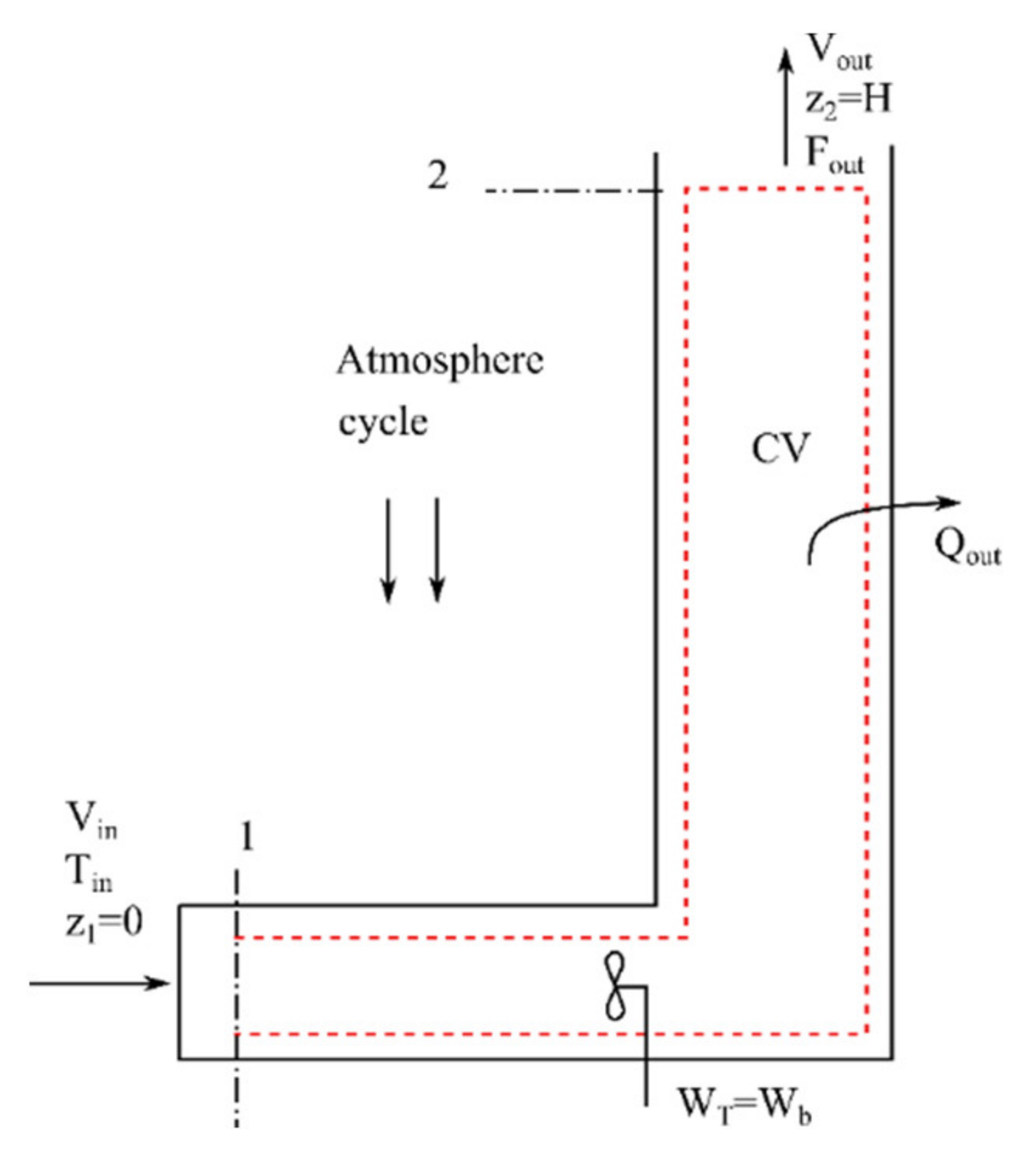
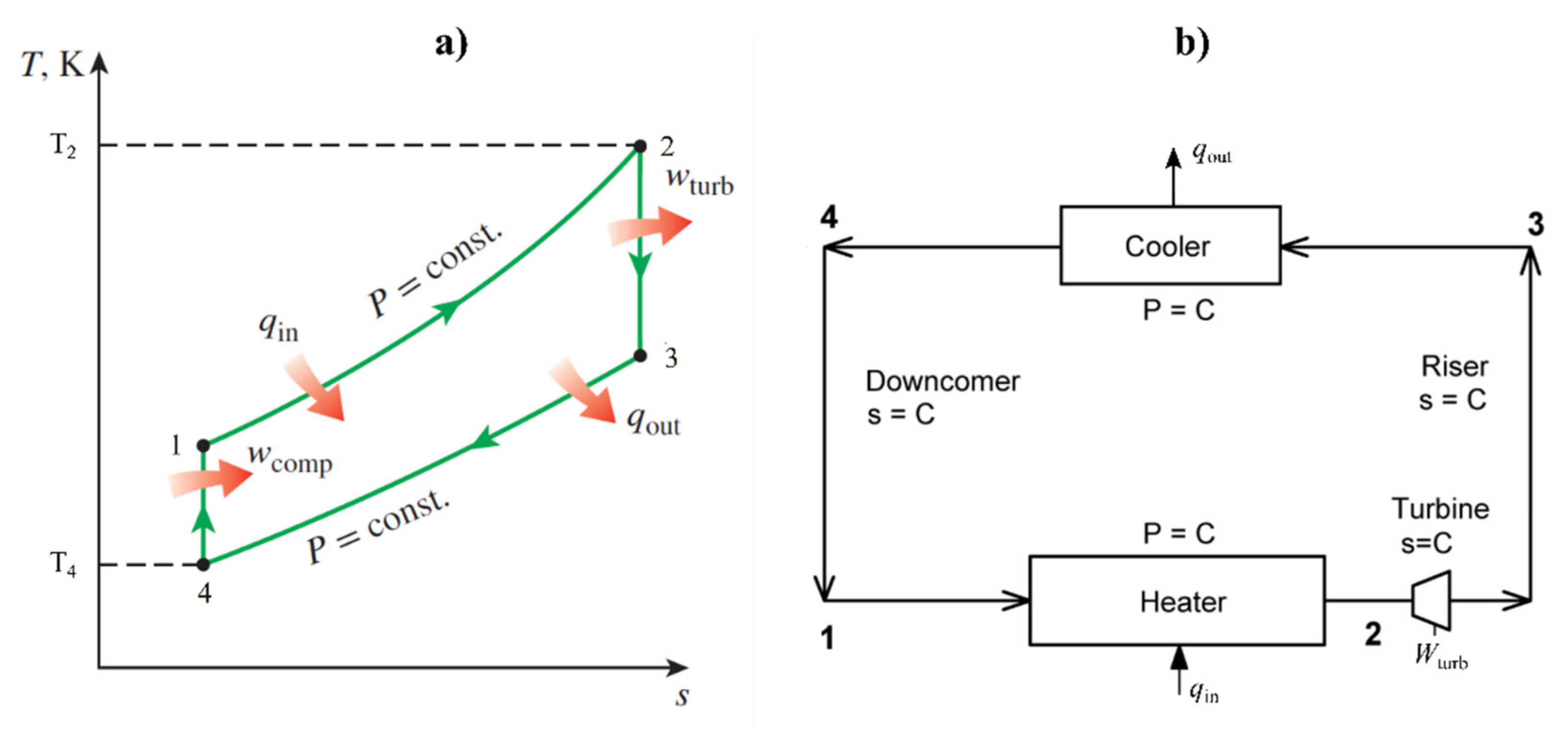
Closed ideal thermodynamic cycles are employed to analyze the atmospheric upward heat convection procedure compared to the particular Brayton gas-turbine cycle [29,31]. Typically, the heat to the work conversion efficiency of the atmosphere is displayed to be close to the Carnot efficiency.

The efficiency is independent of whether or not the lifting process is discontinuous or continuous and almost independent of whether the heat is transported as sensible or latent heat. The T-s diagram of the UVS model based on an ideal Brayton cycle is shown in Figure 26a.

Figure 26b also shows the called gravity power cycle applied for the UVS model. This cycle has the following considerations: the heating and cooling take place at constant pressure, efficiency is a function of pressure ratio only, and the cycle is based on identical Brayton gas turbine cycle except that the expansion and compression take place in vertical conduits instead of in rotating machines [52].

Michaud (1995) showed that the work produced when the heat is carried upward only by convection is equal to the upward heat flux multiplied with the Carnot efficiency calculated utilizing the average temperature at which the heat is received and provided upward. Renno and Ingersoll (1996) independently reached the same conclusion and applied the average temperature from the earth’s surface concerning the hot source temperature and the average temperature from the troposphere for the particular cold source temperature [26].

The work produced when a unit mass of air is expanded adiabatically and reversibly without a chance in elevation is determined by the Equation (16).

$$w=q-\mathsf{\Delta }h-\mathsf{\Delta }gz-\mathsf{\Delta }\frac{V^2}{2}$$

(16)

where w is work; q is heat; h is the enthalpy of the air, including the enthalpy of its water content; g is gravity; z is height; and V is velocity. The heat transfer to and from the fluid in an isentropic expansion process is determined by Equations (17) and (18).

$$q_{in}=h_2-h_1=C_p\left(T_2-T_1\right)$$

(17)

$$q_{out}=h_3-h_4=C_p\left(T_4-T_3\right)$$

(18)

where Cp is the specific heat at constant pressure. The Carnot cycle is the most efficient cycle that can be executed between a heat source at temperature T_.H. and a sink at temperature T_.L., and its thermal efficiency is expressed as:

$${\eta }_{Carnot}=1-\frac{T_L}{T_H}$$

(19)

The work per unit mass, the heat rate contributed by the combustion system, the Carnot efficiency, and the thermal power of the UVS model were determined by solving the previous equations. The thermal power of the prototype was established in a related approach to the procedure used in the model. The initial temperature was calculated from the Carnot efficiency concept. In addition, the inlet velocity of the prototype was calculated based on the dimensionless parameters obtained from the similarity analysis.

The work per unit mass, the heat rate contributed by the combustion system, the Carnot efficiency, and the thermal power of the UVS prototype were determined.

Table 9. Thermal power of UVS model and prototype.

Parameter Name	Parameter Description	Model Value	Prototype Value	Unit
$q_{in}$	Heat received diameter	162.81	8.440	KJ/Kg
$T_{in}$	Inlet temperature	384.5	301.56	K
$V_{in}$	Inlet velocity	2.2	1.75	m/s
${\eta }_{Carnot}$	Carnot efficiency	36	36	%
${\eta }_{UVS}$	UVS efficiency	20	20	%
w	Work per unit mass	58.61	2.985	KJ/Kg
$\dot{m}$	Mass flow rate	0.5	686	Kg/s
$\dot{W}$	Power	29.31	2047.71	KW

summarizes the results obtained.

The results obtained in the model and the prototype agree with the results obtained in AVE experiments [26]. Approximately 20% of the heat received is converted into work during the convection process. It is concluded that a full-scale prototype would have a maximum power of 2 M.W., a specific work of 3 kJ/kg, and raised air at an upward airflow of 6.8 × 10² kg/s.

4.6. Constructive Considerations of the UVS Large-Scale Prototype

The possibility of generating a stable upward vortex flow was demonstrated using a 5-m-high experimental model and a numerical simulation in the sections above. This section analyzes the minimum wind resistance that the VSZ must support in a large-scale prototype. In addition, some ideas for improving the sustainability of the large-scale prototype will be mentioned.

The experimental model and the large-scale prototype are geometrically similar. The linear scale ratio was 1:40 for UVS prototype dimensions, as detailed in Figure 27 and

Table 10. Dimensional specifications for experimental model and UVS prototype.

Parameter Name	Parameter Description	Model Value (m)	Prototype Value (m)
D1	Outer cylinder diameter	4	160
D2	Inner cylinder diameter	3	120
D3	Roof opening diameter	0.8	32
d1	Gap of the fluid inlet	0.4	16
d2	Fluid inlet length	1.5	60
d3	Base thickness	0.3	12
d4	Gap between buildings	0.65	26
d5	VSZ length	2	80
h1	Cylinder height	0.8	32
h2	Fluid inlet height	0.5	20
h3	Building’s height	5	200
R1	Radius of thin-walled blades	0.925	37

.

From these data, it is possible to establish the general measurements of a real application in which four buildings at least 200-m high will be built. These buildings will make up the area (80 m × 80 m) necessary to contain the vortex. The vortex will emerge from a central hole 32 m in diameter, which communicates the VSZ with the vortex generator located underground.

The wind-resistant design plays a significant role in the structural design of the large-scale UVS prototype. Using a wind tunnel study, Yong-Gui Li et al. [53] compared the wind effects on 90° helical and square tall buildings. Their results showed that both designs could withstand a crosswind speed of more than 100 mph (44.7 m/s). Based on the principle of similarity, the calculated wind speed in an actual UVS application was set at 6.1 m/s. Therefore, it is about seven times less than the maximum supported by modern skyscrapers. However, in an optimal design perceptibility, damping and aerodynamic optimization should not be ignored.

As mentioned above, an actual UVS application must have the vortex generator (VG) located underground. It has two advantages. The first advantage is to safeguard the safety of pedestrians because the hot air supply inlet to the VG will be located several meters below the street. The second advantage is to install an automatic control system that guarantees the stability of the created vortex. The control system allows keeping vortex’s stability using the measures of wind velocity and temperatures at various height points in the UVS to regulate the input flow and maintain the stability in the vortex.

If it is impossible to place the VG underground, the winds generated (1.75 m/s) to feed the system will not represent a severe danger for pedestrians. Researchers state that a wind of 1.75 m/s is considered a light breeze, which could cause hair to be disturbed, clothing to flap, and a sense of wind on the face [54,55].

5. Conclusions

In this study, an urban vortex system (UVS) is presented for urban air remediation. Using the commercial CFD software CFX, we established a Reynolds Averaged Navier–Stokes (RANS) simulation with the Renormalized Group (RNG) k– ε turbulence model to evaluate the variations of temperature, velocity, and pressure values. Validation of the numerical results was carried out by comparing the experimental temperature and velocity values. The results reported that a steady-state vortex could be formed when a vapor-air mixture at 2 m/s and 450 K enters the vortex generator. This vortex presented a maximum negative central pressure of −6.81 Pa and a maximum velocity of 5.47 m/s. The simulation deviation standard error was approximately 6%. Therefore, this research concludes that the numerical model tends to give predictions parallel to the experimental data from corresponding tests.

This urban vortex system can generate a stable vortex with an approximately 1.5 m/s updraft wind speed at 400-m high. This speed can break the heat island effect by transporting 686 kg/s of the environment’s warm air to the upper troposphere, thus reducing the heat island effect.

The optimization process of the UVS model was carried out by using the method of goal-driven optimization (GDO). The objective of the UVS model optimization process was to maximize the output parameters corresponding to the velocity and force outputs on the Y-axis as a function of the input parameters that represent the physical conditions of the vapor-air mixture when entering the vortex generator. A candidate point was found by this method, which obtained the best adjustment in the optimization, with a maximum value for the outlet velocity of 1.84 m/s and a maximum value of 6.30 N in the output force. These values are obtained when inserting the steam-air mixture at 2.2 m/s and 384.5 K.

In addition, the principle of similarity between the model and a full-scale prototype indicated that the geometric similarity was achieved by preserving all the angles and dimensions. The kinematic and dynamic similarity was achieved by applying the method of repeating variables. The results obtained from this method were four non-dimensional parameters, which related the resulting buoyancy force to all the variables that were present in the UVS study. Finally, the principle of similarity allowed all the flow characteristics to be transported on a large scale. It is concluded that the proposed large-scale UVS application is predicted to be capable of having a maximum power of 2 M.W., a specific work of 3 kJ/kg, buildings 200-m high, and generating winds of 6.1 m/s (20 km/h) at 200 m up to winds of 1.5 m/s (5 km/h) at 400 m. These winds would cause the rupture of the gas capsule of the heat island phenomenon. Therefore, the city would balance its temperature with that of the surrounding rural areas. However, the practical aspects of the functional design of high-rise buildings are highly recommended to improve the design of UVS.