Operational Performance Evaluation of Korean Ship Parts Manufacturing Industry Using Dynamic Network SBM Model

Abstract

The purpose of this study is to analyze the efficiency and productivity of the Korean ship parts manufacturing industry. To this end, the manufacturing process was divided into two stages (operating activities, financial activities), and the Dynamic Network SBM model and Malmquist Productivity Index were used. We collected analysis data from KIS-VALUE, and analyzed 40 companies from 2014 to 2020. As a result of the analysis, from 2014 to 2017, the average operating efficiency was 0.7825, the average financial efficiency was 0.5208, and the average total efficiency was 0.4537. It was found that improving efficiency requires improving both activities simultaneously, rather than focusing on a specific activity. Operating activities DMI was 1.0025, financial activities DMI was 0.9236, and OMI was 0.9464. In order to improve OMI, it is necessary to improve the financial activities DMI, which is the cause of the decrease in productivity. In order to improve financial activities DMI, government policy or technology change to improve DFS was found to be necessary. Finally, the effect of environmental factors on efficiency was analyzed by tobit regression. It was found that Firm Size had a negative (−) effect on efficiency, and Firm Age had a positive (+) effect on efficiency. The analysis results of this study will help to understand the relationship between input and output, which has been treated as a black box in the manufacturing industry, in two stages; and this will serve as a guideline for those working in Korea’s ship parts manufacturing industry to establish policies.

1. Introduction

Korea’s shipbuilding industry has grown continuously since the 1970s. It has established itself as an important industry, and Korea once recorded the world’s largest share of orders in this industry [1]. However, due to the 2008 financial crisis, the growth in China, and the decline in ship orders, companies in the shipbuilding industry accumulated losses and had to restructure [2,3,4]. Recently, in Korea, the performance of large corporations in the shipping industry has been improving, and the government is actively supporting it [5]. However, the small- and medium-sized enterprises (SMEs) are experiencing a cost burden due to the rise in the price of major raw materials (e.g., steel) [6]. Despite the increase in supply, the actual profit is declining. Additionally, a company has difficulty offering a higher price than its competitors because of the low-bid contract. In Korea, the 52-h workweek system has been implemented not only in large enterprises but also in SMEs with fewer than 50 employees, thus increasing the difficulties in SME management [7]. Compared to other industries, the shipbuilding industry has a high proportion of skilled workers, and most of the salaries of skilled workers come from overtime [8,9]. However, due to the 52-h work system, companies are experiencing difficulties recruiting workforce and feeling the burden of overtime pay for skilled workers, which can lead to the exit of skilled workers. Amid these concerns, R&D for developing eco-friendly ship technology has recently been conducted [10]. Additionally, technology development for smart ships, such as autonomous ships, is in progress [11]. Shipping powerhouses, such as Europe, Japan, and China, are also developing autonomous vessels [12,13]. Moreover, several countries (e.g., Finland, China, and Japan) have already succeeded in testing self-driving ships. As such, the international competition in the shipbuilding industry is becoming fiercer, and the company’s operating activities and financial soundness are of utmost importance [14]. The global shipbuilding market was $162.52 billion in 2019, and decreased to $150.42 billion in 2020 due to COVID-19; however, it is expected to grow annually and recover to 161.83 in 2023, similar to the 2019 level [15]. According to the 2019 OECD Global value chains and the shipbuilding industry report, the shipbuilding industry relies heavily on intermediate inputs and parts, as global shipbuilding orders are 42.74 million GT. Moreover, about 70–80% of the final output value of ship production is generated through the supplier sector [16]. Regarding parts sourcing activities, of the four countries surveyed (i.e., Korea, China, Japan, and EU28), China was the most self-sufficient, followed by Japan and the EU28. Looking at the major trading countries for securing parts by country, we found that China mainly transacted with EU28 and Japan traded mainly with China out of the 4% total imports. Meanwhile, Korea mainly transacted with China out of the 19% total imports, and EU28 mainly traded with Korea out of the 9% of total imports. In 2021, the OECD reported that the Chinese led the global shipbuilding industry for the past 20 years in shipbuilding policy and market developments in selected economies; they accounted for 43.7% of the global shipbuilding industry in 2020 [17]. Moreover, from March 2020 to March 2021, a total of 21 country-specific support policies were investigated, and domestic market protection was supported the most. The frequency of support was highest in China, followed by the United States. Figure 1 shows the annual order volume and market share of countries (Korea, China, and Japan) with a high share of ship orders [18].

The shipbuilding industry is a multi-item, small-volume production system in which few large companies receive parts from SMEs and assemble ships to complete them. Additionally, because the shipbuilding industry is a make-to-order system, the quality of ships is determined by the performance and quality of parts. In Korea’s KIS-VALUE Database, as of 2021, more than 80% of these ship parts manufacturing companies were small and medium-sized enterprises [19,20,21]. Due to the aforementioned 52-h workweek, rising costs, and technological pursuits from competing countries, Korean ship parts manufacturers are experiencing management difficulties [22,23]. Despite the increase in sales, ship parts manufacturer is suffering from production and financial problems due to increasing prices of raw materials and the turnover of skilled workers. Therefore, efficiency and productivity can be important indicators of the performance of ship parts manufacturers. Here, efficiency means the corresponding input/output compared to the optimal input/output, and productivity means the ratio of output to input [24]. To understand the efficiency and productivity of ship parts manufacturing companies, we must look at the operating activities related to manufacturing, sales, and financial aspects concerning financing and redemption as a whole. Data envelopment analysis (DEA) is appropriate for analyzing efficiency and productivity because it can analyze multiple inputs and outputs simultaneously when analyzing efficiency. Several studies have analyzed the efficiency and productivity of various industries [25,26,27]. However, these studies treated the company’s process as a single stage. In other words, prior studies have limitations: they either assume the relationship between inputs and outputs existing within the process as “black box” or fail to consider the linkage of periods (t, t + 1). To overcome the limitations of prior studies, this study applied a dynamic network slack-based measure (DN-SBM) model that can consider the relationship between two-stage constructed inputs and outputs and the linkage between periods (t, t + 1). The DN-SBM model can look at the tradeoff between processes through the link. Additionally, this model enables dynamic analysis that considers situations that affect efficiency and productivity over multiple periods (t, t + 1) through carry-over. In the case of the ship parts manufacturing industry, we must examine both production-related and financial aspects. Our model can analyze efficiency and productivity by separating these aspects and is, therefore, suitable.

This study aims to analyze the efficiency and productivity of the ship parts manufacturing industry. In this study, a DN-SBM model that considers the linkage (t, t + 1) between each process (Stage 1: operating activity; Stage 2: financial activity) and periods was used. Using this model, we analyzed the efficiency and productivity of each process by period and the overall efficiency and productivity. Finally, the effects of environmental factors on efficiency and productivity were analyzed. The analysis results of this study will provide insights for shipbuilding practitioners or policy managers to understand the industry’s business and improve efficiency and productivity. It also provides an improvement direction, that is, which of the processes should be improved first. This may help practitioners allocate an entity’s limited resources efficiently and effectively. Finally, by analyzing the effect of environmental factors on efficiency, this study identifies the efficiency determinants of the ship parts manufacturing industry. These analysis results will help policy practitioners establish policies that consider the environmental characteristics of the enterprise when establishing policies.

2. Literature Review

2.1. Data Envelopment Analysis

The DEA model introduced by Charnes et al. [28] is a nonparametric linear programming method for analyzing the relative efficiency of a decision-making unit (DMU) with multiple inputs and outputs [29,30]. The DEA model has several advantages in efficiency analysis. First, the weights of input and output are calculated to maximize the efficiency of the DMU, so pre-assumption is not necessary. Second, analysis is possible even if multiple inputs and outputs with different units exist. Third, inefficient DMUs are relatively evaluated based on efficient DMUs, and the degree of change in input and output for efficient improvement of inefficient DMUs is shown. The efficiency values are between 1 and 0. Moreover, it can be assumed to be constant returns to scale with the same input and output changes, and variable returns to scale (VRS) with different input and output changes. A VRS is called increasing returns to scale if the change in output is greater than the change in inputs, or decreasing returns to scale (DRS) if the change in inputs is less than the change in output. The most representative models in the DEA model are the CCR model presented by Charnes et al. [28] and the BCC model presented by Banker et al. [31]. However, these models have a limitation in that they measure the efficiency improvement direction radially and do not consider slacks. The SBM model, which belongs to Non-Radial, considers Slacks, which means room for improvement in the input–output, when analyzing efficiency [32]. In the SBM model, the efficient DMU has zero input/output slacks and an efficiency of 1.

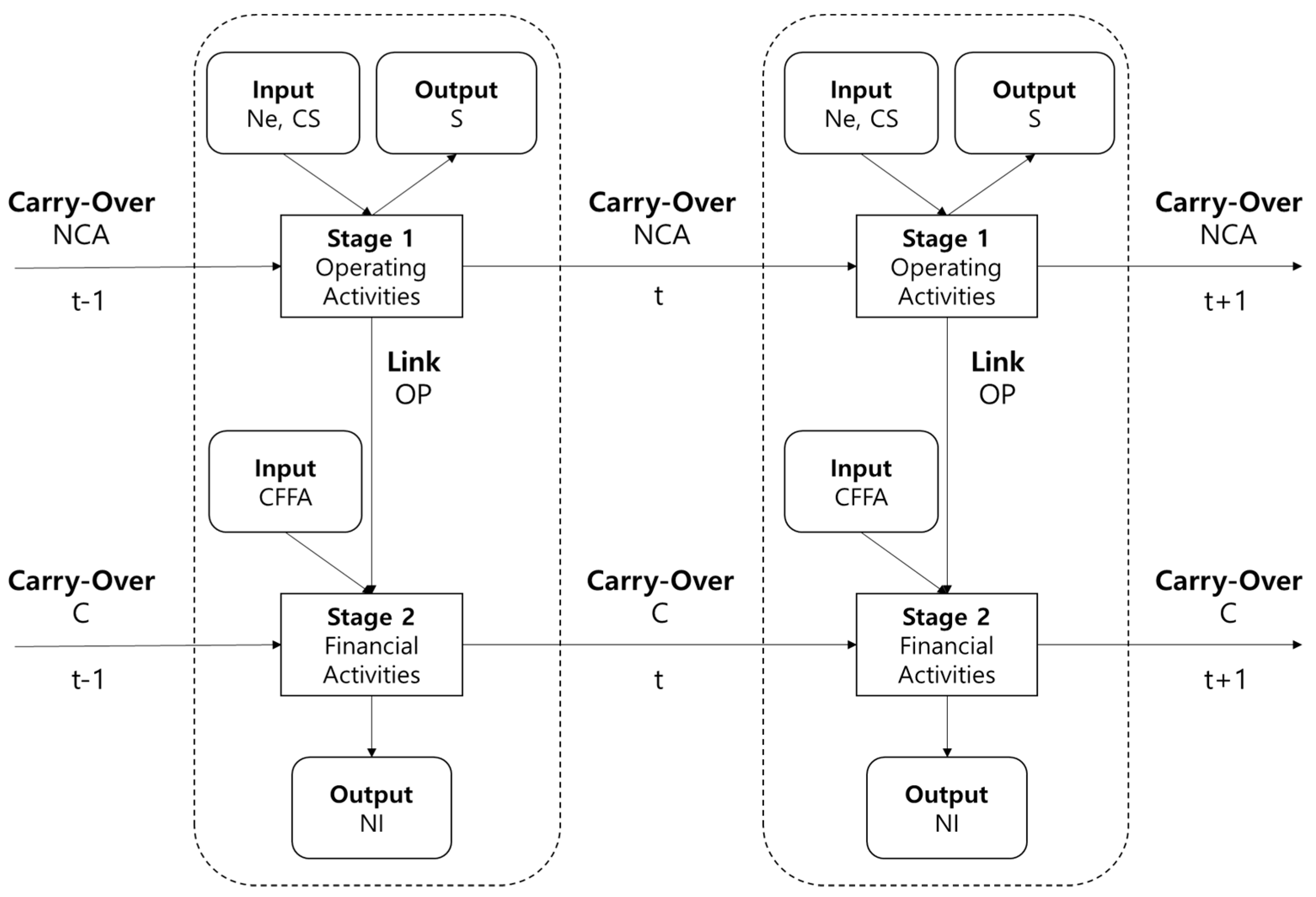
2.2. Dynamic Network SBM Model

The DN-SBM model, presented by Tone and Tsutsui [33], combines the dynamic SBM model’s carry-over and network SBM model’s link. The dynamic SBM model reflects the carry-over activities of consecutive term, which were ignored in existing time series efficiency analysis models (e.g., Window and Malmquist index) [34]. The advantage of the dynamic SBM model is that it reflects long-term quasi-fixed inputs through carry-over, which has the characteristics of preventing biased inefficiency measurements due to static optimization [35]. The following are the four types of carry-over: good, bad, free, and fixed carry-over. Good carry-over means a more desirable variable for the DMU as it carries forward, whereas bad carry-over is the opposite. Meanwhile, free carry-over means a variable connected at discretion, whereas fixed carry-over means a non-discretionary connection that the DMU cannot control. The network SBM model is characterized by considering the black box present in the input/output relationship that was ignored in the existing DEA model via link. This model separates the input/output process into stages and connects each stage through link. Here, link serves as an output in the first stage and as an input in the next stage. If the link that acts as output appears high on the first stage, the efficiency of that stage can be high, but it can be a burden on the next stage. This link acts as an input in stage 2; therefore, it needs that much output to be similar to stage 1’s efficiency. That is, link represents a tradeoff between two stages. Like carry-over, links can be divided into four categories (i.e., good, bad, free, and fixed). These DN-SBM models are non-radial models that consider slacks and are appropriate for the ship parts manufacturing industry consisting of operating and financial activities because they consider carry-over activities and tradeoff.

(a)

The objective function of overall efficiency is

$${\theta }_o^{*}=min\frac{{{\displaystyle \sum }}_{t=1}^T{W}^t\left[{{\displaystyle \sum }}_{k=1}^K{w}^k[1-\frac{1}{m_k+linki{n}_k+nba{d}_k}\left({{\displaystyle \sum }}_{i=1}^{m_k}\frac{S_{iok}^{t-}}{x_{iok}^t}+{{\displaystyle \sum }}_{{\left(k,h\right)}_l=1}^{linki{n}_k}\frac{S_{o{\left(k,h\right)}_{l}in}^t}{z_{o{\left(k,h\right)}_{l}in}^t}+{{\displaystyle \sum }}_{k_l=1}^{nba{d}_k}\frac{S_{o{k}_{l}bad}^{\left(t,t+1\right)}}{z_{o{k}_{l}bad}^{\left(t,t+1\right)}}+\right)]\right]}{{{\displaystyle \sum }}_{t=1}^T{W}^t\left[{{\displaystyle \sum }}_{k=1}^K{w}^k[1-\frac{1}{r_k+linkou{t}_k+ngoo{d}_k}\left({{\displaystyle \sum }}_{i=1}^{r_k}\frac{S_{iok}^{t+}}{y_{iok}^t}+{{\displaystyle \sum }}_{{\left(k,h\right)}_l=1}^{linkou{t}_k}\frac{S_{o{\left(k,h\right)}_{l}out}^t}{z_{o{\left(k,h\right)}_{l}out}^t}+{{\displaystyle \sum }}_{k_l=1}^{ngoo{d}_k}\frac{S_{o{k}_{l}good}^{\left(t,t+1\right)}}{z_{o{k}_{l}good}^{\left(t,t+1\right)}}+\right)]\right]}$$

(1)

with

$$\begin{array}{l}{{\displaystyle \sum }}_{t=1}^T{W}^t=1,{{\displaystyle \sum }}_{k=1}^K{w}^k=1,W^t\ge 0\left(\forall t\right),w^k\ge 0\left(\forall k\right)\hfill \\ \mathrm{s}.\mathrm{t}.x_{ok}^t=X_k^t{\lambda }_k^t+s_{ko}^{t-}\left(k=1,\cdots ,K;t=1,\cdots ,T\right)\hfill \\ y_{ok}^t=Y_k^t{\lambda }_k^t-s_{ko}^{t+}\left(k=1,\cdots ,K;t=1,\cdots ,T\right)\hfill \\ e{\lambda }_k^t=1\left(k=1,\cdots ,K;t=1,\cdots ,T\right)\hfill \\ {\lambda }_k^t\ge 0,s_{ko}^{t-}\ge 0,s_{ko}^{t+}\ge 0\left(\forall k,\forall t\right)\hfill \end{array}$$

(2)

where $X_k^t=\left(x_{1k}^t,\cdots ,x_{nk}^t\right)\in R^{m_k\times n\times T}$ and $Y_k^t=\left(y_{1k}^t,\cdots ,y_{nk}^t\right)\in R^{r_k\times n\times T}$ are input and output matrices, and $s_{ko}^{t-}$ and $s_{ko}^{t+}$ are input/output slacks, respectively. Moreover, ${\lambda }_k^t=\left\{{\lambda }_{jk}^t\right\}\in R_{+}^n$ is the weight of Stage k in period t. If ${{\displaystyle \sum }}_{j=1}^n{\lambda }_{jk}^t=1$, it means variable returns to scale assumption. $Z_{\left(kh\right)free}^t{\lambda }_h^t=Z_{\left(kh\right)free}^t{\lambda }_k^t$ ($\forall \left(k,h\right)free,\forall t)$, $Z_{\left(kh\right)free}^t=\left(z_{1\left(kh\right)free}^t,\cdots ,z_{n\left(kh\right)free}^t\right)\in R^{L_{\left(kh\right)free}\times n}$, $z_{o\left(kh\right)in}^t=Z_{\left(kh\right)in}^t{\lambda }_k^t+s_{o\left(kh\right)in}^t\left(\left(kh\right)in=1,\cdots ,linki{n}_k\right)$. $s_{o\left(kh\right)in}^t\in R^{L_{\left(kh\right)in}}$ is slacks and non-negative, and $linki{n}_k$ is the number of “as input” link from Stage k. $z_{o\left(kh\right)out}^t=Z_{\left(kh\right)out}^t{\lambda }_k^t-s_{o\left(kh\right)out}^t\left(\left(kh\right)out=1,\cdots ,linkou{t}_k\right)$. $s_{o\left(kh\right)out}^t\in R^{L_{\left(kh\right)out}}$ is slacks and non-negative, and $linkou{t}_k$ is the number of “as output” link from Stage k. $W^t\left(t=1,\cdots ,T\right)$ is the weight to period t and $w^k\left(\mathrm{t}=1,\cdots ,K\right)$ is the weight to Stage k.

$n$: Number of DMUs.

T: Number of periods.

$K$: Number of Stages.

$m$: Number of input.

$r$: Number of output.

$x_{ijk}^t$: In period t, Stage k, the i-th input variable of $DM{U}_j$.

$y_{ijk}^t$: In period t, Stage k, the i-th output variable of $DM{U}_j$.

$z_{j{\left(kh\right)}_l}^t$: In period t, the l-th link variable of $DM{U}_j$ from Stage k to Stage h.

$z_{j{k}_l}^{\left(t,\mathrm{t}+1\right)}$: The l-th carry-over variable of Stage k, $DM{U}_j$ from period t to period t + 1.

(b)

Period efficiency (efficiency during period t):

$${\tau }_o^{t^{*}}=\frac{{{\displaystyle \sum }}_{k=1}^K{W}^{\mathrm{k}}\left[1-\frac{1}{m_k+linki{n}_k+nba{d}_k}\left({{\displaystyle \sum }}_{i=1}^{m_k}\frac{s_{iok}^{t-}}{x_{iok}^t}+{{\displaystyle \sum }}_{{\left(k,h\right)}_l=1}^{linki{n}_k}\frac{s_{o{\left(k,h\right)}_{l}in}^t}{z_{o{\left(k,h\right)}_{l}in}^t}+{{\displaystyle \sum }}_{k_l=1}^{nba{d}_k}\frac{s_{o{k}_{l}bad}^{\left(t+t+1\right)}}{z_{o{k}_{l}bad}^{\left(t,t+1\right)}}\right)\right]}{{{\displaystyle \sum }}_{k=1}^K{W}^{\mathrm{k}}\left[1-\frac{1}{r_k+linkou{t}_k+ngoo{d}_k}\left({{\displaystyle \sum }}_{i=1}^{r_k}\frac{s_{iok}^{t+}}{y_{iok}^t}+{{\displaystyle \sum }}_{{\left(k,h\right)}_l=1}^{linkou{t}_k}\frac{s_{o{\left(k,h\right)}_{l}out}^t}{z_{o{\left(k,h\right)}_{l}out}^t}+{{\displaystyle \sum }}_{k_l=1}^{ngoo{d}_k}\frac{s_{o{k}_{l}good}^{\left(t+t+1\right)}}{z_{o{k}_{l}good}^{\left(t,t+1\right)}}\right)\right]}(t=1,\cdots ,T)$$

(3)

(c)

The efficiency of Stage k

$${\delta }_{ok}^{*}=\frac{{{\displaystyle \sum }}_{t=1}^T{W}^t\left[1-\frac{1}{m_k+linki{n}_k+nba{d}_k}\left({{\displaystyle \sum }}_{i=1}^{m_k}\frac{s_{iok}^{t-}}{x_{iok}^t}+{{\displaystyle \sum }}_{{\left(k,h\right)}_l=1}^{linki{n}_k}\frac{s_{o{\left(k,h\right)}_{l}in}^t}{z_{o{\left(k,h\right)}_{l}in}^t}+{{\displaystyle \sum }}_{k_l=1}^{nba{d}_k}\frac{s_{o{k}_{l}bad}^{\left(t+t+1\right)}}{z_{o{k}_{l}bad}^{\left(t,t+1\right)}}\right)\right]}{{{\displaystyle \sum }}_{t=1}^T{W}^t\left[1-\frac{1}{r_k+linkou{t}_k+ngoo{d}_k}\left({{\displaystyle \sum }}_{i=1}^{r_k}\frac{s_{iok}^{t+}}{y_{iok}^t}+{{\displaystyle \sum }}_{{\left(k,h\right)}_l=1}^{linkou{t}_k}\frac{s_{o{\left(k,h\right)}_{l}out}^t}{z_{o{\left(k,h\right)}_{l}out}^t}+{{\displaystyle \sum }}_{k_l=1}^{ngoo{d}_k}\frac{s_{o{k}_{l}good}^{\left(t+t+1\right)}}{z_{o{k}_{l}good}^{\left(t,t+1\right)}}\right)\right]}(k=1,\cdots ,K)$$

(4)

(d)

During period t, the efficiency of Stage k can be expressed as:

$${\rho }_{ok}^{t^{*}}=\frac{1-\frac{1}{m_k+linki{n}_k+nba{d}_k}\left({{\displaystyle \sum }}_{i=1}^{m_k}\frac{s_{iok}^{t-}}{x_{iok}^t}+{{\displaystyle \sum }}_{{\left(k,h\right)}_l=1}^{linki{n}_k}\frac{s_{o{\left(k,h\right)}_{l}in}^t}{z_{o{\left(k,h\right)}_{l}in}^t}+{{\displaystyle \sum }}_{k_l=1}^{nba{d}_k}\frac{s_{o{k}_{l}bad}^{\left(t+t+1\right)}}{z_{o{k}_{l}bad}^{\left(t,t+1\right)}}\right)}{1-\frac{1}{m_k+linkou{t}_k+ngoo{d}_k}\left({{\displaystyle \sum }}_{i=1}^{r_k}\frac{s_{iok}^{t+}}{y_{iok}^t}+{{\displaystyle \sum }}_{{\left(k,h\right)}_l=1}^{linkou{t}_k}\frac{s_{o{\left(k,h\right)}_{l}out}^t}{z_{o{\left(k,h\right)}_{l}out}^t}+{{\displaystyle \sum }}_{k_l=1}^{ngoo{d}_k}\frac{s_{o{k}_{l}good}^{\left(t+t+1\right)}}{z_{o{k}_{l}good}^{\left(t,t+1\right)}}\right)}$$

(5)

2.3. Malmquist Productivity Index

The Malmquist productivity index (MPI) is a common method for measuring changes in productivity over time and was introduced by Malmquist [36,37]. It was developed as a DEA model by Fare et al. [38,39]. MPI can be divided into technical efficiency change index (TECI) and technical change index (TCI) using a distance function without assuming a specific production function. TECI is calculated by dividing the technical efficiency value of t + 1 by the technical efficiency value of t, indicating the degree to which a particular DMU approaches the efficiency frontier between the two periods (t, t + 1). In other words, TECI refers to the extent to which efficiency changes have contributed to productivity changes. Meanwhile, TCI is the geometric average value after evaluating the technological changes of two periods (t, t + 1). TCI refers to the extent to which technological changes in both periods (t, t + 1) contributed to changes in productivity. If the MPI, TECI, and TCI are greater than 1, it means better productivity, better technological efficiency, and advances in technology, respectively. The distinction between TECI and TCI can provide policy implications for productivity improvement. If the TECI is less than 1, policies on introducing and using new technologies that drive catch-up are needed. However, if the TCI is less than 1, a policy is needed to induce technological advancement to move up the efficiency frontier. Accordingly, each stage-specific catch-up and frontier-shift can be represented by expressions (a) and (b). Additionally, MPI by individual and all stages can be represented by expressions (c) and (d), respectively.

(a)

Divisional catch-up index (DCU)

$$DCU={\gamma }_{ok}^{t\to t+1}=\frac{{\rho }_{ok}^{t+1^{*}}}{{\rho }_{ok}^{t^{*}}}\left(t=1,\cdots ,T-1;k=1,\cdots ,K;o=1,\cdots ,n\right)$$

(6)

(b)

Divisional frontier-shift effect

$$DFS={\sigma }_{ok}^{t\to t+1}=\sqrt{{\sigma }_{ok}^t{\sigma }_{ok}^{t+1}}\left(t=1,\cdots ,T-1;k=1,\cdots ,K;o=1,\cdots ,n\right)$$

(7)

(c)

Divisional Malmquist index

$$DMI=DCU\times DFS={\mu }_{ok}^{t\to t+1}={\gamma }_{ok}^{t\to t+1}{\sigma }_{ok}^{t\to t+1}\left(t=1,\cdots ,T-1;k=1,\cdots ,K;o=1,\cdots ,n\right)$$

(8)

(d)

Overall Malmquist index

$$\begin{gathered} OMI={\mu }_o={{\displaystyle \prod }}_{k=1}^K{({\mu }_{ok})}^{w_k} \left(o=1,\cdots ,n\right) \\ {\rho }_{ok}^{t^{*}}:\mathit{efficiency}\mathit{of}DM{U}_o\mathit{at}\mathit{Stage}k\mathit{in}\mathit{period}t \\ {\sigma }_{ok}^t: \mathit{\text{frontier-shift}} \mathit{effect} \mathit{of} DM{U}_o\mathit{at}\mathit{Stage}k\mathit{in}\mathit{period}t \\ {\mu }_{ok}:\mathit{weighted} \mathit{geometric} \mathit{mean} \mathit{of} {\mu }_{ok}^{t\to t+1} \\ {w}_k:\mathit{weight} \mathit{to} \mathit{Stage} k \mathit{with} {{\displaystyle \sum }}_{k=1}^K{w}_k=1 \end{gathered}$$

(9)

3. Research Methodology

3.1. Data and Variables

Ship parts manufacturers, the subject of analysis in this study, selected companies belonging to “ship components manufacturing, C31114” based on the Korea Standard Industrial Classification Code (KSIC). Financial data for 10 years from 2011 to 2020 were collected from the KIS-value database. KIS-VALUE, representing Korea’s financial data, is the largest corporate information database in Korea; it provides financial information on about 20,000 companies since 1980 [21,40]. Therefore, all companies (corporations subject to external audit) that exceed a certain size are included and can represent companies belonging to ship component manufacturing (C31114). To analyze consistent relative efficiency and productivity, companies that went out of business or had missing values in seven years were excluded, leading to 40 companies used in the analysis.

Input and output were selected by referring to the preceding study (

Table 1. References to efficiency and productivity.

Researchers	Analysis Target	Input	Output	Link	Carry-Over
[29]	Indian retailers	1. Cost of labor 2. Capital employed	1. Profit 2. Sales	-	-
[47]	Indian life insurance companies	1. Operating expenses and commissions	1. Premium collected 2. Sum assured	-	1. Investments
[48]	Retail store chains in Canada	1. Capital 2. Number of stores 3. Number of employees 4. Total sales area	1. Sales 2. Profits	-	-
[49]	Iranian airlines	1. Number of employees	1. Passenger-km performed 2. Passenger Ton/km performed	1. Available seat/km 2. Available ton/km 3. Number of scheduled flights	1. The number of fleet’s seat
[50]	Insurance company in Malaysia	1. The operating expenses used in labor and business services	1. Investment Income	1. Incurred claims plus additions to reserves	1. Fixed assets 2. Investment assets
[51]	MENA banking	1. Net loans 2. Total earning assets 3. Non-earning Assets 4. Loan loss prov. 5. Costs	1. Income	1. Net interest Margin 2. Equity 3. Total assets	1. Gross loans 2. Total assets 3. Income

). The process is divided into operational and financial activities because operational activities and financial activities have important interactions [41] and are the main component of tactical management independent of each other [42]. In particular, in the case of Korean manufacturing companies of ship parts, the proportion of small and medium-sized enterprises is high, and they are experiencing difficulties in operation and finance. Thus, the efficiency and productivity of operational and financial activities must be analyzed. Separating operational and finance activities this way has the advantage of analyzing the input–output relationship, which has been treated as a single process, into each activity to determine which activities cause inefficiency and lower productivity. The operational activity is set as Stage 1 to improve management programs, technology, and manufacturing resources, which are key factors for a manufacturing company’s success [43]. Moreover, this is because operational activities, such as manpower, cost of sales, and product sales, affect financial performance [44,45]. Ship parts manufacturers, like general manufacturers, decided that purchasing materials and using human resources and technology to produce and sell products to achieve results took precedence over other activities, so the operation activity was set as the first stage. In other words, we set operating activities, which is the company’s main revenue-generating activity, as Stage 1. Stage 2 was set up as financial activities because the profits from operating activities in ship parts manufacturing companies would lead to financial activities necessary for business operation, such as cash borrowing, repayment, and payment of dividends. Meanwhile, financial activities, a representative indicator of cash liquidity, relate to the performance of an entity [46] and the risk of corporate bankruptcy. This study analyzes the efficiency and productivity of an enterprise through these operating (Stage 1) and financial activities (Stage 2).

In Stage 1, the “number of employees” (NE), “cost of sales” (CS), and “selling and administrative expenses” (S&A) were used as input for operating activities. The number of employees (NE) was selected because skilled and unskilled workers conduct the processes of operating activities (e.g., technology development, product production, and sales). Meanwhile, CS belongs to variable cost and refers to the cost included in manufacturing a product (Beginning inventory of merchandise + Ending inventory of merchandise—Purchase during the year). Lastly, S&A is a fixed cost and includes all operating costs (e.g., salary, training expenses, and rent) that are not included in the cost of sales. For output, sales (S), the result of producing and selling products through CS, and S&A was selected.

Moreover, carry-over, which acts as a quasi-fixed input for consecutive periods, was set as a non-current asset (NCA). This setting is due to NCA’s quasi-fixed characteristic that is difficult to change in a short time as it is an asset that stays with the company for a long period of more than one year. Furthermore, NCA, which includes concepts, such as factories, machines, and patents, can be accumulated for the next period [50]. Meanwhile, operating profit (OP) was used to link Stages 1 and 2. OP is the difference between gross profit (sales-CS) and S&A; it represents the profitability of a business. OP is a representative indicator of profit in terms of operating activities, but it excludes financial activities and does not represent a company’s financial structure. Therefore, in step 2, OP, which is the performance of operating activities, and cash flow from financial activities (CFFA), which represents financing and repayment, are set as inputs. The output was set as net income (NI) after deducting all expenses and losses from income. We also considered Tobin’s Q, but it was excluded from the analysis because of the limitations in calculating the market value due to the nature of the ship parts manufacturing company with a high proportion of SMEs. Finally, carry-over has a quasi-fixed feature and selected capital (C), which means funds raised from shareholders. Stage 1 (operating activities) and Stage 2 (financial activities) are expressed as input, output, link, and carry-over (Figure 2).

3.2. Descriptive Statistics

The descriptive statistics for this study data are shown in

Table 2. Descriptive statistics.

Year		NE	CS	S&A	S	OP	NCA	CFFA	NI	C
2014	AVE	101.9	416.1	43.6	489.5	29.8	432.2	14.3	16.1	250.2
	STDEV	90.7	703.8	33.1	777.4	53.5	633.6	73.2	32.2	338.2
2015	AVE	101.4	420.8	44.7	498.8	33.3	437.1	−6.8	14.0	268.8
	STDEV	86.6	700.3	36.7	782.7	61.4	594.2	59.3	57.7	363.5
2016	AVE	89.4	393.7	46.6	455.7	15.4	444.1	20.3	11.3	283.6
	STDEV	76.3	651.9	43.3	711.0	54.0	590.2	82.8	61.1	403.1
2017	AVE	79.8	284.4	39.1	323.6	0.1	437.2	0.2	−14.2	270.0
	STDEV	71.6	425.5	38.2	463.6	55.6	594.7	40.1	61.4	430.4
2018	AVE	80.6	268.5	31.8	305.9	5.7	442.9	−5.5	−15.9	262.0
	STDEV	70.9	347.5	23.1	380.2	34.5	597.8	58.3	60.3	456.2
2019	AVE	80.3	339.1	34.7	385.2	11.4	441.4	−9.0	−2.5	285.1
	STDEV	74.4	488.7	27.7	526.1	31.6	584.7	74.3	42.3	453.8
2020	AVE	77.8	328.0	34.6	364.7	2.1	450.6	−4.3	−9.2	289.8
	STDEV	69.0	464.2	29.3	496.8	53.4	590.6	39.3	57.6	481.7

NE: Number of employees; CS: Cost of sales; S&A: Selling and administrative expenses; S: Sales; OP: Operating profit; NCA: Non-current assets; CFFA: Cash flow for financial activities; NI: Net income; C: Capital.

. Looking at 2020 (vs. 2014), NE, the input of Stage 1, decreased by 23.7%. Moreover, CS and S&A decreased by 21.2% and 20.6%, respectively. That is, the input of operating activities decreased by about 20%. Moreover, S (i.e., output) and OP (i.e., the link) decreased by 25.5% and 93.0%, respectively, whereas NCA (i.e., carry-over) increased by 4.3%. Meanwhile, CFFA, the input of Stage 2, decreased by 69.9%, and NI, the output, decreased by 42.9%. Lastly, the carry-over C increased by 15.9%.

An isotonicity test was performed to confirm the validity of the model, input, output, link, and carry-over used in this study. The isotonicity test identifies whether an increase in the output occurs with an increase in input [52]. Moreover, if the correlation between variables is positive, using the variable is appropriate [53,54].

Table 3. Correlation matrix of variables.

	NE	CS	S&A	S	OP	NCA	CFFA	NI	C
NE	1
CS	0.733 **	1
S&A	0.734 **	0.642 **	1
S	0.751 **	0.998 **	0.658 **	1
OP	0.510 **	0.615 **	0.221 **	0.656 **	1
NCA	0.595 **	0.805 **	0.402 **	0.796 **	0.488 **	1
CFFA	0.144 *	0.253 **	0.108	0.253 **	0.206 **	0.191 **	1
NI	0.300 **	0.216 **	0.107	0.260 **	0.679 **	0.140 *	0.207 **	1
C	0.722 **	0.576 **	0.492 **	0.593 **	0.489 **	0.711 **	0.071	0.454 **	1

*: p < 0.05, **: p < 0.01. NE: Number of employees; CS: Cost of sales; S&A: Selling and administrative expenses; S: Sales; OP: Operating profit; NCA: Non-current assets; CFFA: Cash flow for financial activities; NI: Net income; C: Capital.

presents the results of correlation analysis on the variables, and positive correlations between all variables were confirmed. The correlation sign of all variables is positive, and most of the correlations are significant; hence, the use of the variables in this study is considered valid [55].

4. Analysis Results

4.1. Empirical Results of the Dynamic Network DEA

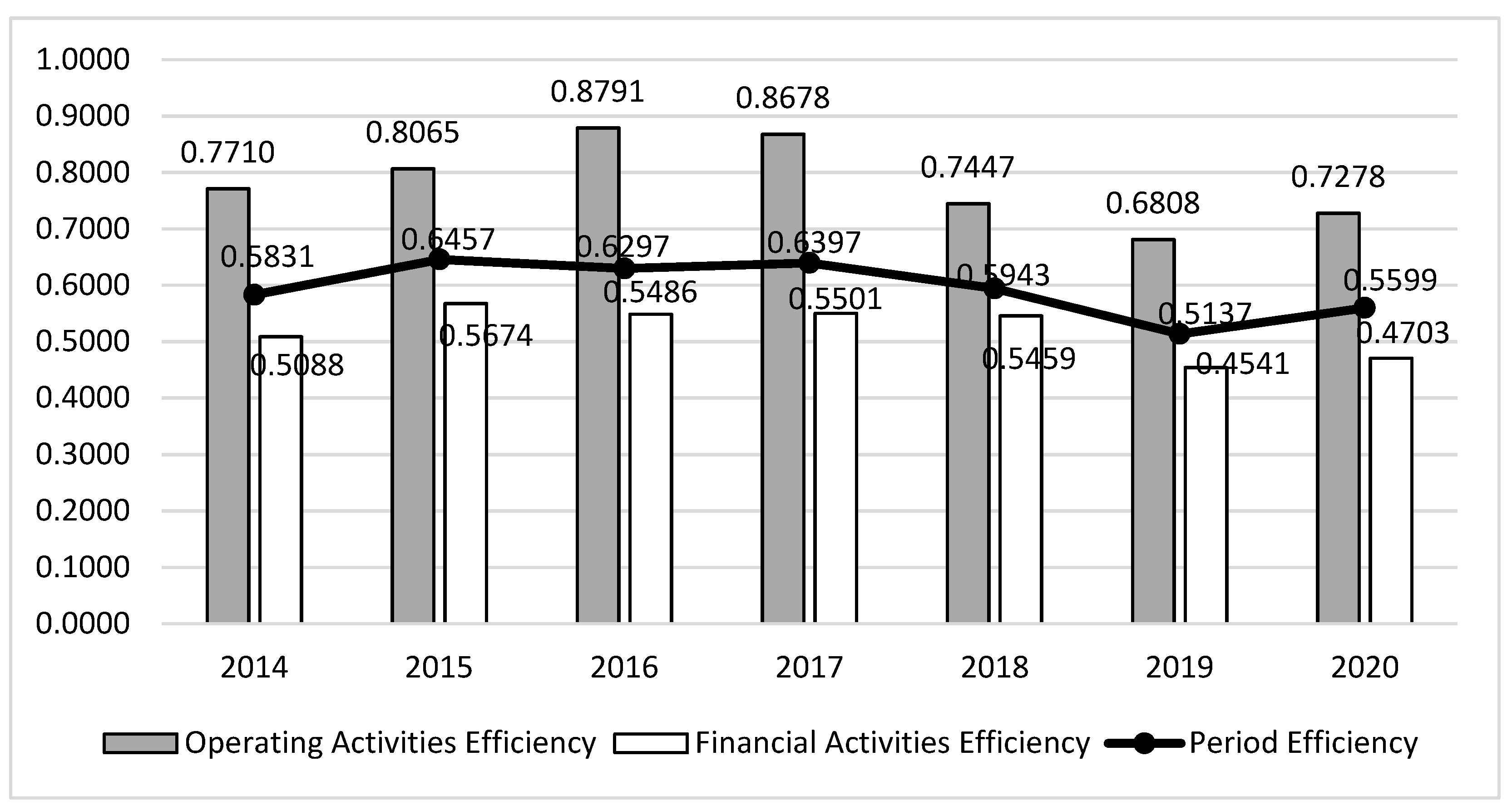
4.1.1. Operating Activity (Stage 1) Efficiency

This study analyzes the efficiency of the management processes of Korean ship parts manufacturing companies by dividing them into operating activities (Stage 1) and financial activities (Stage 2).

Table 4. The efficiency of operating activities (Stage 1) by period.

DMU No.	Overall Efficiency Rank	OA Efficiency Rank	Overall Efficiency	OA Efficiency
				2014	2015	2016	2017	2018	2019	2020
1	1	1	1	1	1	1	1	1	1	1
2	1	1	1	1	1	1	1	1	1	1
3	3	1	0.9999	1	1	1	1	1	1	1
4	4	1	0.9992	1	1	1	1	1	1	1
5	5	12	0.9866	0.8171	1	1	1	1	1	1
6	6	1	0.8978	1	1	1	1	1	1	1
7	7	15	0.8274	0.9996	1	0.9996	0.9999	0.9999	0.9980	0.3254
8	8	14	0.6923	1	1	1	1	0.7306	0.7084	1
9	9	17	0.6731	1	0.7500	0.7500	0.7500	0.7500	1	0.7500
10	10	18	0.6508	1	1	1	1	0.6274	0.5403	0.5610
11	11	20	0.6414	1	1	1	0.8477	0.7056	0.6751	0.4386
12	12	16	0.6329	1	1	1	1	1	0.3737	0.4609
13	13	1	0.5913	1	1	1	1	1	1	1
14	14	1	0.5836	1	1	1	1	1	1	1
15	15	29	0.5086	0.5720	0.7540	0.8282	1	0.5562	0.3986	0.4133
16	16	24	0.4741	0.4750	0.5724	0.6642	0.6370	1	1	0.6614
17	17	33	0.4566	0.3795	0.1427	0.7101	0.7700	0.7717	0.8000	0.6375
18	18	1	0.4441	1	1	1	1	1	1	1
19	19	27	0.4117	0.6173	0.7010	0.5364	0.8179	0.4758	0.6772	1
20	20	34	0.3731	0.5925	0.6711	0.5274	0.8928	0.9859	0.1865	0.2507
21	21	26	0.3597	0.4933	0.5648	0.8676	0.9546	0.9999	0.5329	0.5069
22	22	1	0.3380	1	1	1	1	1	1	1
23	23	22	0.3348	0.9584	1	1	0.7887	0.7104	0.2018	0.6804
24	24	19	0.3264	0.7700	1	1	1	0.8396	0.0693	1
25	25	32	0.3216	0.5080	0.9535	1	0.3497	0.3994	0.4431	0.5738
26	26	40	0.3076	0.3537	0.3945	0.5650	0.4209	0.3503	0.4751	0.5451
27	27	1	0.2955	1	1	1	1	1	1	1
28	28	13	0.2623	0.7232	0.8372	1	0.9987	0.9350	1	1
29	29	30	0.2472	0.7444	1	1	0.9997	0.1575	0.2542	0.2490
30	30	36	0.2347	0.8298	0.3550	0.5795	1	0.4090	0.3554	0.2092
31	31	21	0.2245	1	1	1	1	1	0.4876	0.1736
32	32	31	0.2112	0.3882	0.6400	0.8230	0.7175	0.6102	0.4474	0.7296
33	33	1	0.1769	1	1	1	1	1	1	1
34	34	35	0.1760	0.7144	0.7279	0.7317	0.6147	0.0650	0.1568	0.7757
35	35	37	0.1394	0.3528	0.0989	0.5810	0.5950	0.6026	0.5947	0.6323
36	36	25	0.1226	0.6680	0.6053	0.9694	0.8025	1	0.1646	0.7211
37	37	39	0.0745	0.4640	0.6405	0.5665	0.2124	0.0193	0.4515	0.9743
38	38	28	0.0652	0.3825	0.2964	0.7672	0.9301	0.3440	1	1
39	39	23	0.0611	0.5465	1	1	0.9997	0.2203	0.8337	0.6867
40	40	38	0.0248	0.4907	0.5560	0.6974	0.6110	0.5212	0.4063	0.1559
AVE			0.4537	0.7710	0.8065	0.8791	0.8678	0.7447	0.6808	0.7278
MAX			1	1	1	1	1	1	1	1
MIN			0.0248	0.3528	0.0989	0.5274	0.2124	0.0193	0.0693	0.1559
STDEV			0.2962	0.2456	0.2648	0.1709	0.2043	0.3058	0.3198	0.2890

presents the analysis result of operating activities (Stage 1) by period. From 2014 to 2020, the number of companies that operate efficiently during the entire period in Stage 1 was 11. In 2016, the highest number of companies that operated efficiently by period was recorded at 23, whereas in 2018 and 2019, the lowest number of 16 was recorded. The average efficiency over seven years is 0.7825, and the standard deviation is 0.1844. Moreover, the average efficiency in 2020 (vs. 2014) deteriorated by 5.6%, and the average standard deviation increased by 17.7%. Looking at the operating activities in 2020 (Stage 1) compared to 2014, we determined that the efficiency deteriorated, and the standard deviation increased. This result means that the gap between efficient and inefficient firms is becoming wider.

4.1.2. Financial Activities Stage (Stage 2) Efficiency

The analysis results of the efficiency of financial activities (Stage 2) by period are shown in

Table 5. The efficiency of financial activities (Stage 2) by period.

DMU No.	Overall Efficiency Rank	FA Efficiency Rank	Overall Efficiency	FA Efficiency
				2014	2015	2016	2017	2018	2019	2020
1	1	1	1	1	1	1	1	1	1	1
2	1	1	1	1	1	1	1	1	1	1
3	3	4	0.9999	1	1	0.9998	0.9987	1	1	1
4	4	5	0.9992	1	1	1	1	0.9908	0.9986	1
5	5	1	0.9866	1	1	1	1	1	1	1
6	6	6	0.8978	0.9524	1	0.7850	0.3889	1	1	1
7	7	7	0.8274	0.9998	0.9464	0.4939	0.9957	0.9996	0.9997	0.6697
8	8	22	0.6923	0.9999	1	0.6027	0.3011	0.1095	0.1931	0.0353
9	9	19	0.6731	0.5000	0.5000	0.5000	0.5000	0.5000	0.5000	0.5000
10	10	12	0.6508	0.2865	0.4727	0.9432	0.5001	1	0.5241	0.6472
11	11	17	0.6414	0.4430	1	0.3007	0.7712	0.0998	0.5529	0.5267
12	12	14	0.6329	1	0.7801	0.7234	0.5257	0.3875	0.1965	0.6021
13	13	8	0.5913	0.0598	1	1	1	0.9963	1	0.9998
14	14	27	0.5836	0.3014	0.3098	0.3230	0.3236	0.6291	0.4465	0.2774
15	15	20	0.5086	0.2331	0.3023	0.8933	0.8743	0.5701	0.2196	0.3290
16	16	16	0.4741	0.0719	0.5403	0.8366	0.5007	1	0.5285	0.5181
17	17	9	0.4566	0.1207	1	1	1	1	0.9995	0.5855
18	18	28	0.4441	1	0.2921	0.2099	0.2317	0.1640	0.3332	0.1763
19	19	30	0.4117	0.4639	0.1631	0.2206	0.3500	0.1795	0.0552	0.7611
20	20	10	0.3731	0.8579	0.9001	0.1156	0.9945	0.9789	0.6293	0.1772
21	21	26	0.3597	0.0861	0.1781	0.6377	0.2892	1	0.1384	0.3680
22	22	25	0.3380	0.2165	0.1443	0.0592	0.8745	0.8540	0.3905	0.3490
23	23	23	0.3348	0.4872	0.4866	1	0.3242	0.0688	0.2850	0.4518
24	24	18	0.3264	1	1	1	0.1176	0.1174	0.1911	0.0963
25	25	15	0.3216	0.2827	0.7956	1	0.8535	0.1019	0.0680	0.9302
26	26	32	0.3076	0.1699	0.1990	0.6948	0.0627	0.5045	0.1943	0.3059
27	27	38	0.2955	0.0993	0.2845	0.0922	0.1149	0.1951	0.1574	0.2353
28	28	11	0.2623	0.0828	0.4806	0.0315	1	1	1	1
29	29	33	0.2472	0.2833	0.4199	0.0782	0.3570	0.1273	0.2512	0.1412
30	30	40	0.2347	0.2147	0.0844	0.1844	0.1765	0.0776	0.0635	0.0292
31	31	13	0.2245	1	0.9636	0.1792	0.9686	0.9809	0.1078	0.0301
32	32	35	0.2112	0.2861	0.3028	0.3996	0.1130	0.1431	0.0801	0.0794
33	33	36	0.1769	0.1548	0.0938	0.0325	0.0705	0.1293	0.6147	0.2451
34	34	21	0.1760	0.6912	1	1	0.4602	0.0890	0.1073	0.0334
35	35	39	0.1394	0.0667	0.0950	0.1373	0.4392	0.2202	0.0087	0.1949
36	36	31	0.1226	0.9351	0.3537	0.6373	0.1504	0.0516	0.0214	0.0251
37	37	37	0.0745	0.0610	0.0857	0.1450	0.1014	0.3566	0.0125	0.5329
38	38	34	0.0652	0.0373	0.0982	0.0224	0.0130	0.0310	0.8155	0.5003
39	39	24	0.0611	0.2541	0.2962	0.4755	0.9999	0.5283	0.0038	0.4536
40	40	29	0.0248	0.6535	0.1288	0.1900	0.2613	0.6562	0.4749	0.0031
AVE			0.4537	0.5088	0.5674	0.5486	0.5501	0.5459	0.4541	0.4703
MAX			1	1	1	1	1	1	1	1
MIN			0.0248	0.0373	0.0844	0.0224	0.0130	0.0310	0.0038	0.0031
STDEV			0.2962	0.3823	0.3666	0.3752	0.3622	0.3981	0.3726	0.3473

. From 2014 to 2020, three companies operated efficiently, with an average efficiency of 0.5208 and a standard deviation of 0.2703. The number of companies that operate efficiently by period was highest in 2016 and 2018 with 3, and the lowest in 2017, 2019, and 2020 with 7. Compared to 2014, the efficiency in 2020 decreased by 7.6%, and the standard deviation decreased by 9.2%. Moreover, financial activities by period (Stage 2) had lower efficiency than operating activities (Stage 1), and the standard deviation was large.

4.1.3. Periodic and Overall Efficiency

Figure 3 presents operating activity (Stage 1), financial activity (Stage 2), and period efficiency. As shown in the figure, the efficiency of financial activity is always lower than that of operating activity. Moreover, in 2015 and 2016, despite the improved efficiency of operating activities, the efficiency of the financial activities and periodic efficiency deteriorated. Conversely, despite the deterioration in the efficiency of operating activities in 2016 and 2017, the efficiency of financial activities was improved, thereby enhancing the period efficiency. These results reveal that, to improve the period efficiency of ship parts manufacturing companies, business activities that produce and sell products must be operated efficiently, capital must be raised, and financial activities must be repaid. Although the period efficiency was strengthened due to an improvement in financial activities efficiency in 2017, the efficiency of both operating and financial activities decreased in 2018 and 2019, thereby decreasing period efficiency. However, in 2020, the efficiency of both sales and financial activities improved, thus improving period efficiency. This result shows that to improve the period efficiency of ship parts manufacturers, they must improve the two stages equally without a bias between stages.

Table 6. Period efficiency and overall efficiency.

DMU No.	Overall Efficiency Rank	Overall Efficiency	2014	2015	2016	2017	2018	2019	2020
1	1	1	1	1	1	1	1	1	1
2	1	1	1	1	1	1	1	1	1
3	3	0.9999	1	1	0.9999	0.9994	1	1	1
4	4	0.9992	1	1	1	1	0.9954	0.9993	1
5	5	0.9866	0.9072	1	1	1	1	1	1
6	6	0.8978	0.9756	1	0.8925	0.5861	1	1	1
7	7	0.8274	0.9997	0.9727	0.7383	0.9978	0.9998	0.9988	0.4544
8	8	0.6923	0.9999	1	0.8014	0.6505	0.4510	0.4755	0.5177
9	9	0.6731	0.8333	0.6250	0.6250	0.6250	0.6250	0.8333	0.6250
10	10	0.6508	0.4564	0.6450	0.9716	0.7500	0.8137	0.5322	0.6041
11	11	0.6414	0.6150	1	0.5913	0.8094	0.4087	0.6140	0.4827
12	12	0.6329	1	0.8765	0.8617	0.7629	0.6580	0.2796	0.5272
13	13	0.5913	0.1454	1	1	1	0.9981	1	0.9999
14	14	0.5836	0.6121	0.5889	0.4883	0.4979	0.7961	0.6639	0.5709
15	15	0.5086	0.4172	0.5323	0.8608	0.9356	0.5635	0.3083	0.3633
16	16	0.4741	0.1476	0.5548	0.7504	0.5689	1	0.7642	0.5898
17	17	0.4566	0.1649	0.3056	0.8551	0.8850	0.8858	0.8997	0.6115
18	18	0.4441	1	0.5515	0.3541	0.4046	0.2817	0.5191	0.5023
19	19	0.4117	0.5503	0.3438	0.3878	0.4914	0.3648	0.2030	0.8806
20	20	0.3731	0.6991	0.7720	0.1898	0.9435	0.9825	0.2562	0.2106
21	21	0.3597	0.1716	0.3086	0.7569	0.5348	1	0.2053	0.4193
22	22	0.3380	0.3659	0.3537	0.1118	0.9368	0.9270	0.5827	0.6549
23	23	0.3348	0.7240	0.7395	1	0.4418	0.1184	0.2262	0.5716
24	24	0.3264	0.8850	1	1	0.2119	0.4785	0.0779	0.5482
25	25	0.3216	0.3874	0.8663	1	0.4971	0.1881	0.1152	0.7520
26	26	0.3076	0.2216	0.2479	0.6299	0.2418	0.4274	0.3347	0.4255
27	27	0.2955	0.2446	0.4429	0.1706	0.2745	0.3524	0.4085	0.4424
28	28	0.2623	0.2388	0.6704	0.0611	0.9994	0.9675	1	1
29	29	0.2472	0.4748	0.7081	0.1457	0.6784	0.1489	0.2527	0.1904
30	30	0.2347	0.5409	0.2033	0.4036	0.5457	0.3112	0.2306	0.0916
31	31	0.2245	1	0.9815	0.3935	0.9843	0.9904	0.2185	0.0507
32	32	0.2112	0.3287	0.4610	0.5941	0.1890	0.2210	0.1304	0.1429
33	33	0.1769	0.2680	0.2368	0.0629	0.1449	0.3668	0.8074	0.4522
34	34	0.1760	0.7028	0.8640	0.8658	0.5374	0.0743	0.1419	0.0669
35	35	0.1394	0.1132	0.0985	0.3592	0.5028	0.3163	0.0453	0.4311
36	36	0.1226	0.8016	0.4830	0.8040	0.3153	0.0982	0.0363	0.1172
37	37	0.0745	0.2749	0.3702	0.3495	0.1834	0.0279	0.0349	0.7557
38	38	0.0652	0.0853	0.1412	0.0424	0.0260	0.0532	0.9077	0.7502
39	39	0.0611	0.4001	0.5807	0.7309	0.9998	0.2905	0.0101	0.5869
40	40	0.0248	0.5721	0.3014	0.3394	0.4361	0.5887	0.4335	0.0053
AVE		0.4537	0.5831	0.6457	0.6297	0.6397	0.5943	0.5137	0.5599
MAX		1	1	1	1	1	1	1	1
MIN		0.0248	0.0853	0.0985	0.0424	0.0260	0.0279	0.0101	0.0053
STDEV		0.2962	0.3230	0.2982	0.3259	0.3012	0.3524	0.3583	0.3031

presents the results of period and overall efficiency, in which operating activities (Stage 1) and financial activities (Stage 2) are combined. Two companies were found to have operated efficiently for the entire period from 2014 to 2020. The overall efficiency, which combines all stages and periods, is 0.4537, and the standard deviation is 0.2962. The number of efficient companies by period was the largest in 2015 with 10, and the lowest was in 2017 with 5. Based on 2014, period efficiency in 2020 decreased by 4.0%, and the standard deviation decreased by 6.2%.

Through the analysis of external factors affecting the efficiency, additional implications for efficiency improvement of ship parts manufacturers were presented. To this end, we performed Tobit regression [56,57], the dependent variable was set as the overall efficiency, and the independent variable was set as firm size (large companies, SMEs), firm age, regional location, and regional GDP. The analysis results are shown in

Table 7. Tobit regression analysis results.

	Estimate	Std. Error	T-Value	Pr(>t)
Intercept	0.368	0.200	1.843	0.065
Firm Size	−0.308	0.139	−2.220	0.026 *
Firm Age	0.012	0.006	2.102	0.036 *
Region	0.052	0.105	0.493	0.622
GDP	0.000	0.000	0.757	0.449
logSigma	−1.296	0.116	−11.149	0.000 ***

*: p < 0.05, ***: p < 0.001.

. Findings reveal that the company size has a negative effect on the overall efficiency, whereas the company age has a positive effect on the overall efficiency.

4.2. Empirical Results of the Malmquist Productivity Index

Efficiency measures whether an input produces as much as it can technically produce, whereas productivity refers to the ratio of output to input. The two words are similar but different concepts. Even if a company operates efficiently, productivity may be lower than that of a company that operates inefficiently. Conversely, even a highly productive company can operate inefficiently, and even an efficient company can further increase productivity. Therefore, productivity and efficiency must be examined simultaneously. MPI is an index indicating the change in productivity. MPI can be divided into TECI, which means the degree to which changes in technological efficiency contributed to productivity changes, and TCI, indicating the degree to which changes in technology contributed to changes in productivity. TECI, TCI, and MPI for each stage were expressed as DCU, DFS, and DMI. Moreover, the MPI for all stages was expressed as OMI. The MPI analysis results are shown in

Table 8. MPI analysis result.

DMU No.	OMI Rank	OMI	OA (Stage 1)			FA (Stage 2)
			DCU	DFS	DMI	DCU	DFS	DMI
1	25	0.8621	1	1.0299	1.0299	1	0.7217	0.7217
2	3	1.2536	1	1.7592	1.7591	1	0.8933	0.8933
3	11	1.0819	1	1.2076	1.2076	1	0.9693	0.9692
4	31	0.7919	1	0.9200	0.9200	1	0.6816	0.6816
5	38	0.6786	1.0342	1	1.0342	1	0.4450	0.4453
6	28	0.8500	1	1.0216	1.0216	1.0082	0.7016	0.7073
7	23	0.8898	0.8294	0.9911	0.8220	0.9354	1.0298	0.9633
8	34	0.7182	1	0.9361	0.9361	0.5728	0.9618	0.5510
9	16	0.9763	0.9532	1	0.9532	1	1	1
10	13	1.0241	0.9082	0.9638	0.8753	1.1455	1.0462	1.1983
11	21	0.9089	0.8717	0.9522	0.8300	1.0293	0.9669	0.9952
12	30	0.7941	0.8789	0.9536	0.8381	0.9189	0.8188	0.7525
13	4	1.2400	1	0.9615	0.9616	1.5991	1	1.5989
14	29	0.8127	1	0.8790	0.8790	0.9863	0.7619	0.7514
15	24	0.8843	0.9473	0.9127	0.8645	1.0591	0.8541	0.9046
16	6	1.2168	1.0567	1.0039	1.0608	1.3898	1.0044	1.3958
17	1	1.5242	1.0903	1.0443	1.1385	1.3011	1.5684	2.0407
18	20	0.9272	1	1.3286	1.3286	0.7488	0.8642	0.6471
19	14	1.0195	1.0837	1.0375	1.1244	1.0860	0.8511	0.9244
20	33	0.7487	0.8665	1.0246	0.8877	0.7688	0.8214	0.6315
21	19	0.9293	1.0045	1.0015	1.0060	1.2739	0.6738	0.8584
22	18	0.9470	1	1.0789	1.0789	1.0828	0.7676	0.8312
23	17	0.9642	0.9445	1.0553	0.9968	0.9875	0.9444	0.9326
24	36	0.7011	1.0445	0.8549	0.8929	0.6770	0.8131	0.5505
25	12	1.0406	1.0205	0.9978	1.0183	1.2196	0.8719	1.0634
26	9	1.1049	1.0747	1.0023	1.0772	1.1030	1.0275	1.1333
27	10	1.0876	1	0.9068	0.9068	1.1546	1.1296	1.3044
28	5	1.2176	1.0555	1.0898	1.1503	1.5147	0.8509	1.2889
29	26	0.8584	0.8332	1.0346	0.8620	0.8904	0.9600	0.8548
30	35	0.7101	0.7948	0.9879	0.7852	0.7171	0.8956	0.6422
31	39	0.6255	0.7469	1.0752	0.8031	0.5577	0.8735	0.4872
32	27	0.8546	1.1109	0.9623	1.0691	0.8076	0.8458	0.6831
33	15	1.0176	1	0.9590	0.9591	1.0796	1	1.0797
34	32	0.7821	1.0138	1	1.0138	0.6035	1	0.6034
35	8	1.1548	1.1021	1.0215	1.1258	1.1957	0.9905	1.1845
36	37	0.6942	1.0128	0.9492	0.9614	0.5472	0.9159	0.5012
37	7	1.1964	1.1316	0.8814	0.9973	1.4351	1	1.4352
38	2	1.3231	1.1737	0.9677	1.1358	1.5414	1	1.5414
39	22	0.8942	1.0388	0.9233	0.9591	1.1014	0.7568	0.8336
40	40	0.5494	0.8260	1.0041	0.8295	0.4099	0.8861	0.3639
AVE		0.9464	0.9862	1.0170	1.0025	1.0112	0.9041	0.9236
MAX		1.5242	1.1737	1.7592	1.7591	1.5991	1.5684	2.0407
MIN		0.5494	0.7469	0.8549	0.7852	0.4099	0.4450	0.3639
STDEV		0.2111	0.0953	0.1470	0.1726	0.2795	0.1694	0.3551

. First, the average DMI, DCU, and DFS of operating activities (Stage 1) is 1.0025, 0.9862, and 1.0170, respectively. This can be seen as an increase in productivity due to DFS despite the decrease in productivity due to DCU. The average DMI of financial activities (Stage 2) is 0.9236, DCU is 1.0112, and DFS is 0.9041. Although DCU of financial activities (vs. operating activities) contributed to productivity increase, DFS decreased productivity, and, thus, productivity of financial activities decreased. The combined OMI of the productivity of operating activities and that of financial activities is 0.9464. This can be seen because of the decrease in productivity of financial activities despite the increase in productivity of operating activities.

5. Discussion

This study analyzed the efficiency and productivity of Korean ship parts manufacturing companies by dividing them into operating and financial activities. The academic implications of this study are as follows. First, management processes that were previously treated as black boxes in ship parts manufacturing companies were divided into operating and financial activities, and the linkage of the period was considered. In studies using the existing DEA model, the relationship between input and output was treated as only one stage [29,47,48]. This method does not reflect the tradeoff in the input–output relationship. Moreover, although the existing Window and Malmquist studies analyzed the efficiency and productivity by period, a limitation exists because the linkage between periods is not reflected [58]. These limitations focus on maximizing efficiency in each period; therefore, a distortion exists in the efficiency analysis [34]. However, this study analyzed the efficiency by dividing the management process that was treated as a black box into operating and financial activities through the DN-SBM model, reflecting the linkage between tradeoff characteristics and periods. Second, the TECI and TCI for operating and financial activities were analyzed with the MPI based on the DN-SBM model. The existing MPI analysis did not consider the link between the black box and period [59]. However, in this study, MPI analysis was performed based on the DN-SBM model. Through this, we can determine the cause of the decrease in productivity of ship parts manufacturers and suggest activities that urgently need improvement. Third, the external variables affecting efficiency are analyzed through Tobit regression. Efficiency can be improved at the firm level, but it can also be affected by external environmental factors [26]. By analyzing the effect of external variables on efficiency, this study suggests a direction to reflect external environmental characteristics when developing policies to improve efficiency.

The practical implications are as follows. First, by analyzing the efficiency of business and financial activities, this study suggested the most necessary activities to improve the total efficiency. According to the Financial Stability Report of the Bank of Korea, the interest coverage rate of Korean shipbuilders, which represents the ability of a company to meet interest expenses, as of 2019 was less than 100%, indicating that the debt cannot be repaid with profits [25]. In this study, the average operating activities efficiency and the average financial activity efficiency were 0.7825 and 0.5208, respectively, indicating that financial activity efficiency improvement needs to be implemented first. As a method of improving the efficiency of financing activities, a lean production method exists, which has the advantage of improving quality and financial savings [60]. Moreover, balanced improvement of operating and financial activities by period is necessary through the change in period efficiency. If attention is focused only on improving the efficiency of certain activities during sales and financial activities, the balance may be disturbed. To improve business and financial activities in a balanced way, firms must find and improve the cause of inefficiency in detail using the Balanced Scorecard [61]. Second, MPI analysis was performed on operating and financial activities. From these analysis results, we can determine which activities should be improved first to improve OMI. Korea’s Gross Tonnage was 14.6 in 2018, 21.7 in 2019, and 18.1 in 2020, showing decreased productivity [62]. Results of this study reveal that OMI was less than 1, indicating a decrease in productivity. To improve this, we must improve the productivity of financial activities. Moreover, to improve the productivity of financial activities, we must improve the technical change for financial activities. To this end, the loan method of policy financial institutions (e.g., the export–import method of Bank of Korea) and external institutions related to the finance of ship parts manufacturers, such as government-supported projects, must be changed. In particular, the relationship between banks and SMEs positively affects corporate performance [63], and banks need to understand ship parts manufacturers. For example, if a policy financial institution provides funds to shipping companies in the form of direct loans, Korean shipbuilders can maintain financial soundness by increasing ship exports while not increasing debt. For government-related policy, the government should induce technical changes related to financial activities through ship funds or financial consulting to easily issue a refund guarantee. Third, by analyzing external variables that affect efficiency, the policy direction for improving efficiency according to the characteristics of the external environment was presented. The Tobit regression analysis results reveal that company size harmed the overall efficiency, whereas company age positively affected the overall efficiency. Moreover, studies exploring the efficiency of manufacturing companies in East Africa found that company size and efficiency had a negative (−) effect, and in R&D commercialization efficiency, SMEs showed higher efficiency than large companies, showing similarities [64,65]. This means that to improve efficiency in a rapidly changing business environment, companies should continue developing technology, preventing the departure of skilled workers, managing inventory, and securing financial soundness, rather than increasing the external size of the company. If these activities are continued, the technology will accumulate, and financial soundness will improve, thereby improving the company’s efficiency.

6. Conclusions

6.1. Summary of Results

This study analyzed the efficiency and productivity of Korean ship parts manufacturing companies for seven years from 2014 to 2020. For this purpose, the management process of ship parts manufacturing companies was divided into operating activities (Stage 1) and financial activities (Stage 2). As an analysis tool, the DN-SBM model among the DEA models and the MPI based on this model were used. The number of companies used in the analysis was 40, and the average operating activities efficiency of ship parts manufacturing companies was 0.7825. Moreover, the average financial activity efficiency is 0.5208, and the average overall efficiency is 0.4537. Two companies were found to have operated efficiently for seven years from 2014 to 2020. The MPI analysis results reveal that the DMI, that is, the MPI of operating activities, is 1.0025, and the DMI, that is, the MPI of financial activities, is 0.9236. Moreover, the OMI, which stands for MPI that combines these DMIs, showed a decrease in productivity at 0.9464. To identify problems related to efficiency and productivity improvement, firms must identify which stage efficiency and productivity are low. For example, if the efficiencies of Stages 1 and 2 are 0.9 and 0.8, respectively, Stage 2 must be improved first. Methods to improve efficiency reduce input and increase output. Moreover, to improve productivity, firms must preferentially improve the lowest value among DCU and DFS. If the DCU is low, the efficiency aspect should be improved, and if the DFS is low, the external aspects (technology development, machine adoption, policy) should be improved. In this study’s efficiency, improvement of both the efficiency and DFS of financial activities was found to be urgent. In other words, to improve efficiency and productivity, financial activities must be improved. To this end, rather than expanding the scale of ship parts manufacturing companies, they must secure financial soundness through debt repayment and improve operating activities, such as cost of sales management, in a balanced way. Moreover, to improve productivity, changes in the external environment and companies are required, and government policies, such as direct loans from financial institutions and the provision of financial consulting, must be provided by the government. As of 2020, when comparing gross tonnage, which indicates productivity, with China and Japan, Korea ranked second with 18.1, China with 23.2, and Japan with 12.8 [64]. We compared the capacity of the Korean shipbuilding industry with China, Japan, and Europe. In 2021, the capacity of the Korean shipbuilding industry was 11.5, the second-highest after China (14), and the expected capacity in 2022 would still be lower than that of China (13) [66].

6.2. Limitations and Future Study

The limitations of this study are as follows. First, efficiency and productivity were analyzed only with financial data. Future research needs to design a model that more reflects the characteristics of ship parts manufacturers by using non-financial data (e.g., number of patents, technology level). In particular, technology is important in the ship parts industry, and not reflecting this aspect is the study’s limitation.

Second, only Korean ship parts manufacturing companies were analyzed. In the shipbuilding industry, Korea has a high market share and excellent technological prowess, but competing countries (e.g., Japan and China) are also significant. This study analyzed only Korean companies; therefore, the relative effectiveness of Korean companies in the shipbuilding parts industry in global countries is unknown. Therefore, in future research, the efficiency and productivity must be analyzed by collecting data of globally excellent companies.

Third, when analyzing the external environment that affects the efficiency, stakeholders must analyze legal aspects, such as environmental regulations. Currently, advanced countries are developing technologies to manufacture ships made of eco-friendly materials or to minimize pollution. This situation may be an active challenge for companies to consider the environment voluntarily, or it may result from government policies or pressure from the international community. Therefore, in the future, the efficiency and productivity of the shipbuilding industry must be studied considering the government’s policy or global interest.

Fourth, in this study, the efficiency and productivity reflecting the characteristics of manufacturing companies were analyzed by dividing corporate activities into operating activities and financial activities. However, the analysis of investment activities, which is the activity of acquiring or disposing of facility assets to be used for a long time based on the funds secured by a company, is insufficient. Therefore, efficiency and productivity must be measured in future research by adding variables for investment activities and developing activities that integrate three stages or financial and investment activities.

Fifth, in terms of operational activities, the characteristics of the manufacturing network structure have important implications for network operations, such as production decision-making, product recall, and consensus formation. Therefore, future studies need to provide a foundation for efficient operation decision-making of manufacturing companies by analyzing interaction and attribute metrics (i.e., relational functions and node functions) within the network, which are important for evaluating the industry’s operational performance.

Finally, for a more detailed analysis of future efficiency and productivity, a questionnaire (e.g., AHP) asking practitioners the importance of each input/output must be designed. AHP analysis results can be used as input/output weights [67], and efficiency and productivity analysis can be performed, reflecting the characteristics of reality.

References

1. Tan, S.K. Race in the Shipbuilding Industry: Cases of South Korea, Japan and China. Int. J. East Asian Studies 2017, 6, 65–81. [Google Scholar] [CrossRef]
2. Lee, T.T.; Han, J.K. Optimal Korea’s Government Organization of Shipping and Shipbuilding. Asian J. Ship. Logis. 2018, 34, 234–239. [Google Scholar] [CrossRef]
3. Chung, D.; Shin, D. When do firms invest in R&D? Two types of performance feedback and organizational search in the Korean shipbuilding industry. Asian Bus. Manag. 2021, 20, 583–617. [Google Scholar]
4. Business Korea. Big Drop in Number of Skilled Shipbuilding Workforce Feared to Erode the Industry Base. 2018. Available online: http://www.businesskorea.co.kr/news/articleView.html?idxno=20369 (accessed on 24 January 2018).
5. Maeil Business News Korea. Korean Shipbuilders Gain Full Govt Blessing for Global Dominance, Stocks Rise. 2021. Available online: https://pulsenews.co.kr/view.php?sc=30800028&year=2021&no=875065 (accessed on 10 September 2021).
6. The Korea Times. Raw Material Price Increases Could Burden Korea’s Economy. 2021. Available online: https://www.koreatimes.co.kr/www/nation/2021/09/488_314728.html?fl (accessed on 30 August 2021).
7. Park, S.Y.; Lee, D.H. The Effects of CEO’s Compassionate Rationalism Leadership Strategies on Innovation Activities and Business Performance in SMEs. J. Soc. Korea Ind. Syst. Eng. 2019, 42, 70–79. [Google Scholar] [CrossRef]
8. Vietnam News. Shipbuilding Industry Short of Skilled Workers. 2019. Available online: https://vietnamnews.vn/society/536283/shipbuilding-industry-short-of-skilled-workers.html (accessed on 3 October 2019).
9. Newsdirectory3. I Can’t Work Overtime, So My Monthly Salary is Reduced by 100,000 won… Runs from Two-Job to Three-Job. 2021. Available online: https://www.newsdirectory3.com/i-cant-work-overtime-so-my-monthly-salary-is-reduced-by-100000-won-runs-from-two-job-to-three-job/ (accessed on 12 September 2021).
10. Offshore Energy. South Korea Unveils Initiative to Promote Eco-Friendly Ship Technologies—Offshore Energy (Offshore-Energy.Biz); Navingo: Schiedam, The Netherlands, 2020. [Google Scholar]
11. Netherlands Enterprise Agency. Development of Autonomous Ship technologies in Korea; Netherlands Enterprise Agency: AL Den Haag, The Netherlands, 2019. [Google Scholar]
12. The Economist. As Crews Grow Old, Japanese Shipping Firms Try to Do without Them as Crews Grow Old, Japanese Shipping Firms Try to Do without Them; The Economist: London, UK, 2020. [Google Scholar]
13. Globenewswire. Global Autonomous Ships Market (2020 to 2030)—Increasing Use of Automated Systems to Reduce Human Errors and Risks is Driving Growth. 2021. Available online: https://www.globenewswire.com/en/news-release/2021/01/21/2162032/28124/en/Global-Autonomous-Ships-Market-2020-to-2030-Increasing-Use-of-Automated-Systems-to-Reduce-Human-Errors-and-Risks-is-Driving-Growth.html (accessed on 21 January 2021).
14. Wada, Y.; Hamada, K.; Hirata, N. Shipbuilding capacity optimization using shipbuilding demand forecasting model. J. Mar. Sci. Technol. 2021. [Google Scholar] [CrossRef]
15. Martin, P. Size of the Global Shipbuilding Market in 2019 with a Forecast for 2020 through 2023; Statista: Hamburg, Germany, 2021. [Google Scholar]
16. OECD. Global Value Chains and the Shipbuilding Industry; OECD Publishing: Paris, France, 2019. [Google Scholar]
17. OECD. Shipbuilding Policy and Market Developments in Selected Economies; OECD Publishing: Paris, France, 2021. [Google Scholar]
18. Korea Offshore & Shipbulding Association. 2020. Available online: http://www.koshipa.or.kr/ (accessed on 2 January 2020).
19. Lyu, J.; Gunasekaran, A. Design for quality in the shipbuilding industry. Int. J. Qual. Rel. Manag. 1993, 10, 57–64. [Google Scholar] [CrossRef]
20. Li, H.; Womer, K. Optimizing the supply chain configuration for make-to-order manufacturing. Eur. J. Oper. Res. 2012, 221, 118–128. [Google Scholar] [CrossRef]
21. KISVALUE. 2021. Available online: https://www.kisvalue.com/web/index.jsp (accessed on 2 January 2021).
22. The Korea Herald, Last Straw—Application of 52-Hour Workweek Adds to Difficulties Faced by Small Businesses. 2021. Available online: http://www.koreaherald.com/view.php?ud=20210608000960 (accessed on 9 June 2021).
23. Korea JoongAng Daily. 52-Hour Workweek Continues to Create Headaches. 2019. Available online: https://koreajoongangdaily.joins.com/2019/07/07/economy/52hour-workweek-continues-to-create-headaches/3065212.html (accessed on 7 July 2019).
24. Grosskopf, S. Efficiency and Productivity, the Measurement of Productive Efficiency: Techniques and Applications; Oxford University Press: New York, NY, USA, 1993. [Google Scholar]
25. Lee, J.S. Directions for the sustainable development of Korean small and medium sized shipyards. Asian J. Ship. Logis. 2013, 29, 335–336. [Google Scholar] [CrossRef]
26. Park, J.; Lee, D.; Zhu, J. An integrated approach for ship block manufacturing process performance evaluation: Case from a Korean shipbuilding company. Int. J. Prod. Econ. 2014, 156, 214–222. [Google Scholar] [CrossRef]
27. Choi, Y.; Yu, Y.; Lee, H.S. A study on the sustainable performance of the steel industry in Korea based on SBM-DEA. Sustainability 2018, 10, 173. [Google Scholar] [CrossRef] [Green Version]
28. Charnes, A.; Cooper, W.W.; Rhodes, E. Measuring the efficiency of decision-making units. Eur. J. Oper. Res. 1978, 2, 429–444. [Google Scholar] [CrossRef]
29. Gandhi, A.; Shankar, R. Efficiency measurement of Indian retailers using data envelopment analysis. Int. J. Ret. Dist. Manag. 2014, 42, 500–520. [Google Scholar] [CrossRef]
30. Goyal, J.; Kaur, H.; Aggarwal, A. Investigating the Technical and Scale Efficiencies of Indian Textile Industry: A Target Setting Based Analysis Through DEA. IUP J. Oper. Manag. 2017, 16, 16–38. [Google Scholar]
31. Banker, R.D.; Charnes, A.; Cooper, W.W. Some models for estimating technical and scale inefficiencies in data envelopment analysis. Manag. Sci. 1984, 30, 1078–1092. [Google Scholar] [CrossRef] [Green Version]
32. Tone, K. Variations on the theme of slacks-based measure of efficiency in DEA. Eur. J. Oper. Res. 2010, 200, 901–907. [Google Scholar] [CrossRef] [Green Version]
33. Tone, K.; Tsutsui, M. Dynamic DEA with network structure: A slacks-based measure approach. Omega 2014, 42, 124–131. [Google Scholar] [CrossRef] [Green Version]
34. Tone, K.; Tsutsui, M. Dynamic DEA: A slacks-based measure approach. Omega 2010, 38, 145–156. [Google Scholar] [CrossRef] [Green Version]
35. Guo, X.; Lu, C.C.; Lee, J.H.; Chiu, Y.H. Applying the dynamic DEA model to evaluate the energy efficiency of OECD countries and China. Energy 2017, 134, 392–399. [Google Scholar] [CrossRef]
36. Malmquist, S. Index numbers and indifference surfaces. Trab. Estadística 1953, 4, 209–242. [Google Scholar] [CrossRef]
37. Akbarian, D. Overall profit Malmquist productivity index under data uncertainty. Fin. Innov. 2020, 6, 6. [Google Scholar] [CrossRef] [Green Version]
38. Fare, R.; Färe, R.; Fèare, R.; Grosskopf, S.; Lovell, C.K. Production Frontiers; Cambridge University Press: New York, NY, USA, 1994. [Google Scholar]
39. Karimi, B.; Davtalab-Olyaie, M.; Abdali, A.A. A suitable business model for bank branches: Combining business model and Malmquist Productivity Index (MPI). Bus. Econ. J. 2018, 9, 348. [Google Scholar] [CrossRef]
40. Lee, C.; Cho, H.; Lee, D. The mechanism of innovation spill-over across sub-layers in the ICT industry. Asian J. Technol. Innov. 2021, 29, 159–179. [Google Scholar] [CrossRef]
41. Ravid, S.A. On interactions of production and financial decisions. Fin. Manag. 1988, 17, 87–99. [Google Scholar] [CrossRef]
42. Siminica, M.; Motoi, A.G.; Dumitru, A. Financial management as component of tactical management. Pol. J. Manag. Stud. 2017, 15, 206–217. [Google Scholar] [CrossRef]
43. Roth, A.V.; Miller, J.G. Success factors in manufacturing. Bus. Hor. 1992, 35, 73–82. [Google Scholar] [CrossRef]
44. Wayhan, V.B.; Werner, S. The impact of workforce reductions on financial performance: A longitudinal perspective. J. Manag. 2000, 26, 341–363. [Google Scholar] [CrossRef]
45. Hofer, C.; Eroglu, C.; Hofer, A.R. The effect of lean production on financial performance: The mediating role of inventory leanness. Int. J. Prod. Econ. 2012, 138, 242–253. [Google Scholar] [CrossRef]
46. Lundholm, R.; Serafeim, G.; Yu, G. FIN around the world: The contribution of financing activity to profitability. Harv. Bus. Sch. Work. Paper Ser. 2012, 13-011, 1–50. [Google Scholar] [CrossRef] [Green Version]
47. Sinha, R.P. A dynamic DEA model for Indian life insurance companies. Glob. Bus. Rev. 2015, 16, 258–269. [Google Scholar] [CrossRef]
48. Takouda, P.M.; Dia, M. Relative efficiency of hardware retail stores chains in Canada. Int. J. Oper. Res. 2016, 27, 275–290. [Google Scholar] [CrossRef]
49. Omrani, H.; Soltanzadeh, E. Dynamic DEA models with network structure: An application for Iranian airlines. J. Air Trans. Manag. 2016, 57, 52–61. [Google Scholar] [CrossRef]
50. Tone, K.; Kweh, Q.L.; Lu, W.M.; Ting, I.W. Modeling investments in the dynamic network performance of insurance companies. Omega 2019, 88, 237–247. [Google Scholar] [CrossRef]
51. Wanke, P.; Azad, M.A.; Emrouznejad, A.; Antunes, J. A dynamic network DEA model for accounting and financial indicators: A case of efficiency in MENA banking. Int. Rev. Econ. Fin. 2019, 61, 52–68. [Google Scholar] [CrossRef] [Green Version]
52. Goshime, Y.; Kitaw, D.; Jilcha, K. Lean manufacturing as a vehicle for improving productivity and customer satisfaction: A literature review on metals and engineering industries. Int. J. Lean Six Sigma 2019, 10, 691–714. [Google Scholar] [CrossRef]
53. Wanke, P.; Tsionas, M.G.; Chen, Z.; Antunes, J.J. Dynamic network DEA and SFA models for accounting and financial indicators with an analysis of super-efficiency in stochastic frontiers: An efficiency comparison in OECD banking. Int. Rev. Econ. Fin. 2020, 69, 456–468. [Google Scholar] [CrossRef]
54. Avkiran, N.K. An application reference for data envelopment analysis in branch banking: Helping the novice researcher. Int. J. Bank Mark. 1999, 17, 206–220. [Google Scholar] [CrossRef]
55. Udhayakumar, A.; Charles, V.; Kumar, M. Stochastic simulation based genetic algorithm for chance constrained data envelopment analysis problems. Omega 2011, 39, 387–397. [Google Scholar] [CrossRef]
56. Kuo, K.C.; Lu, W.M.; Dinh, T.N. Firm performance and ownership structure: Dynamic network data envelopment analysis approach. Manag. Decis. Econ. 2020, 41, 608–623. [Google Scholar] [CrossRef]
57. Hoff, A. Second stage DEA Comparison of approaches for modelling the DEA score. Eur. J. Oper. Res. 2007, 181, 425–435. [Google Scholar] [CrossRef]
58. Deng, F.; Xu, L.; Fang, Y.; Gong, Q.; Li, Z. PCA-DEA-tobit regression assessment with carbon emission constraints of China’s logistics industry. J. Clean. Prod. 2020, 271, 122548. [Google Scholar] [CrossRef]
59. Li, N.; Liu, C.; Zha, D. Performance evaluation of Chinese photovoltaic companies with the input-oriented dynamic SBM model. Renew. Energy 2016, 89, 489–497. [Google Scholar] [CrossRef]
60. The Korean Economic Daily. Korea’s Only Shipyard under Creditor Protection to Be Sold This Year. 2021. Available online: https://www.kedglobal.com/newsView/ked202107300013 (accessed on 30 July 2021).
61. Kaplan, R.S.; Norton, D.P. The balanced scorecard: Measures that drive performance. Harv. Bus. Rev. 2005, 83, 172. [Google Scholar]
62. Unctadstat. Ships Built by Country of Building. 2021. Available online: https://unctadstat.unctad.org/wds/TableViewer/tableView.aspx?ReportId=89493 (accessed on 31 March 2021).
63. Hoshi, T.; Kashyap, A.; Scharfstein, D. The role of banks in reducing the costs of financial distress in Japan. J. Fin. Econ. 1990, 27, 67–88. [Google Scholar] [CrossRef]
64. Aggrey, N.; Eliab, L.; Joseph, S. Firm size and technical efficiency in East African manufacturing firms. Curr. Res. J. Econ. Theory 2010, 2, 69–75. [Google Scholar]
65. Chun, D.; Chung, Y.; Bang, S. Impact of firm size and industry type on R&D efficiency throughout innovation and commercialisation stages: Evidence from Korean manufacturing firms. Technol. Anal. Strateg. Manag. 2015, 27, 895–909. [Google Scholar]
66. Statista. Global Shipbuilding Capacity from 2013 to 2020, with a Forecast for 2021 through 2026, by Country. 2021. Available online: https://www.statista.com/statistics/1256561/global-shipbuilding-capacity-by-country/ (accessed on 11 August 2021).
67. Lai, P.L.; Potter, A.; Beynon, M.; Beresford, A. Evaluating the efficiency performance of airports using an integrated AHP/DEA-AR technique. Transp. Policy 2015, 42, 75–85. [Google Scholar] [CrossRef]
Figure 1. Ship orders and market share by country.
Sustainability 13 13127 g001
Figure 2. Research model.
Sustainability 13 13127 g002
Figure 3. Efficiency of each stage and the period.
Sustainability 13 13127 g003