
Integrated Optimization of Line Planning, Timetabling and Rolling Stock Allocation for Urban Railway Lines


Abstract
1. Introduction
- (1)
- The formulation of a succinct integrated model to achieve the simultaneous optimization of line planning, timetabling and rolling stock allocation based on a prior set of candidate trips. It has the simplified decisions of selecting some candidate trips for operation, and further assigning their arrival/departure times and service rolling stock.
- (2)
- The proposal of a solution approach based on a metaheuristic-type solver namely a simulated annealing algorithm to solve the integrated model then a test of the performance of the formulated model using the data of Xian metro line 1.
2. Literature Review
3. Methods and Materials
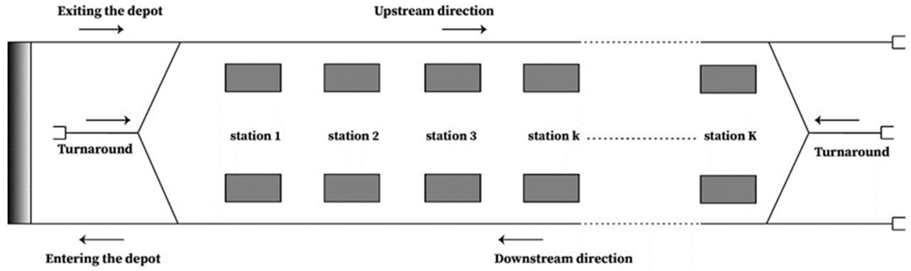
3.1. Problem Description
- 1.
- Only one rolling stock can enter a station at a time,
- 2.
- Only full-length services are taken into account i.e., each servicing trip travels from one terminal station all the way to the other terminal station,
- 3.
- Overtaking operations are not considered i.e., each service trip stops at each station on its path,
- 4.
- There are no limits for parking rolling stock in the depot,
- 5.
- The formation and capacity of rolling stock are considered fixed forming a carrying capacity,
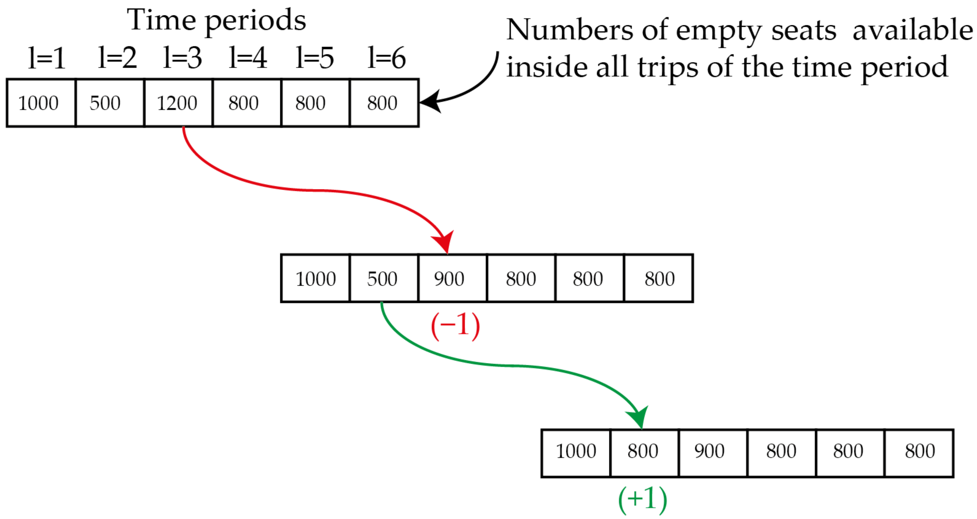
3.2. The Assignment of a Trip’s Service Passengers Based on Queuing Theory
3.3. Model Formulation
3.4. Solution Approach
| Algorithm 1. Randomized solution search. |
| Initialization Set Randomized search corresponds to peak hours: Then set ; ; Otherwise check if Equations (1)/(2) are verified Then check if Then verify whether and set ; ; Otherwise set ; ; Otherwise check whether and set ; ; Otherwise set ; ; Otherwise set ; Calculate |
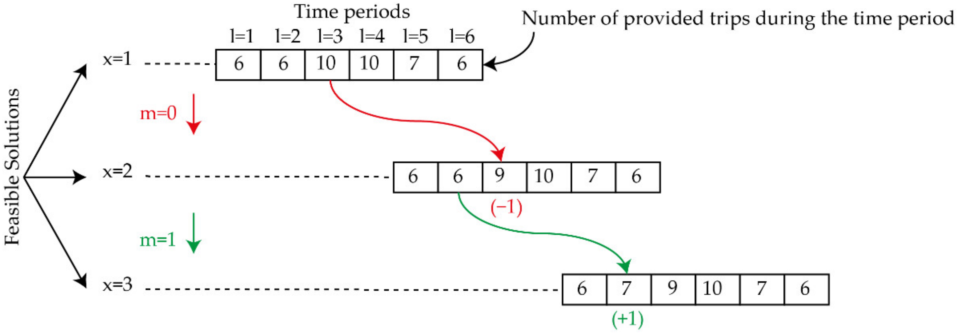
| Algorithm 2. Neighbor solution search. |
| Set ; ; Check if Then set; Find and set as the prioritized time period Find the last provided trip in the time period and set; Otherwise set; Find and set as the prioritized time period Find the first none provided trip in the time period and set ; Calculate |
| Algorithm 3. Passenger flow assignment and timetabling. |
| Calculate / based on Check if Equations (3) and (4) is verified: Keep value Otherwise set:;/; Calculate /: Based on Equations (31) and (32) if/ Based on Equations (33) and (34) otherwise Calculate : Based on Equations (29) and (30) if / Based on Equations (27) and (28) otherwise Calculate based on Equations (35) and (36) Calculate based on Equations (39) and (40) Calculate based on Equations (37) and (38) Calculate based on Equations (41) and (42) Calculate based on Equations (7) and (8) Recalculate based on Equations (9) and (10) using Calculate / based on Equations (5) and (6) Check if Equations (3) and (4) is verified: Keep value Otherwise set:;/; |
| Algorithm 4. Rolling stock allocation. |
| If : Check if (22) is verified: Set:; ; ; Check if (24) is verified: Keep value Otherwise: calculate based on Equation (24) Otherwise, if (22) is not verified: ;; Check if (20), (17) are verified: Keep ; Otherwise set:; ; ; If : Check if Equation (21) is verified Set ; Check if Equation (23) is verified: Maintain value Otherwise calculate based on Equation (23) Otherwise set ; Check if (18), (19) are verified: Keep ; Otherwise set:; If : Check if Equations (11)–(14) are verified Keep values of / Otherwise recalculate / based on the Equations Calculate / based on Equations (25) and (26) |
| Algorithm 5. Calculation of the objective function and termination of inner and outer cycles. |
| Calculating the objective function Calculate based on Equation (45) Calculate based on Equation (46) Calculate based on Equation (47) Calculate / based on Equations (43) and (44) Calculate based on Equations (48)–(51) Algorithm termination Determining optimal solution Check if : Then set Otherwise check if then set; Otherwise check if : Then set Otherwise set Termination of inner-cycle Check if : Then go to termination of outer-cycle Otherwise set and go to Algorithm 2 Termination of outer-cycle Check if : Then set go to Algorithm 2 Otherwise terminate algorithm and display |
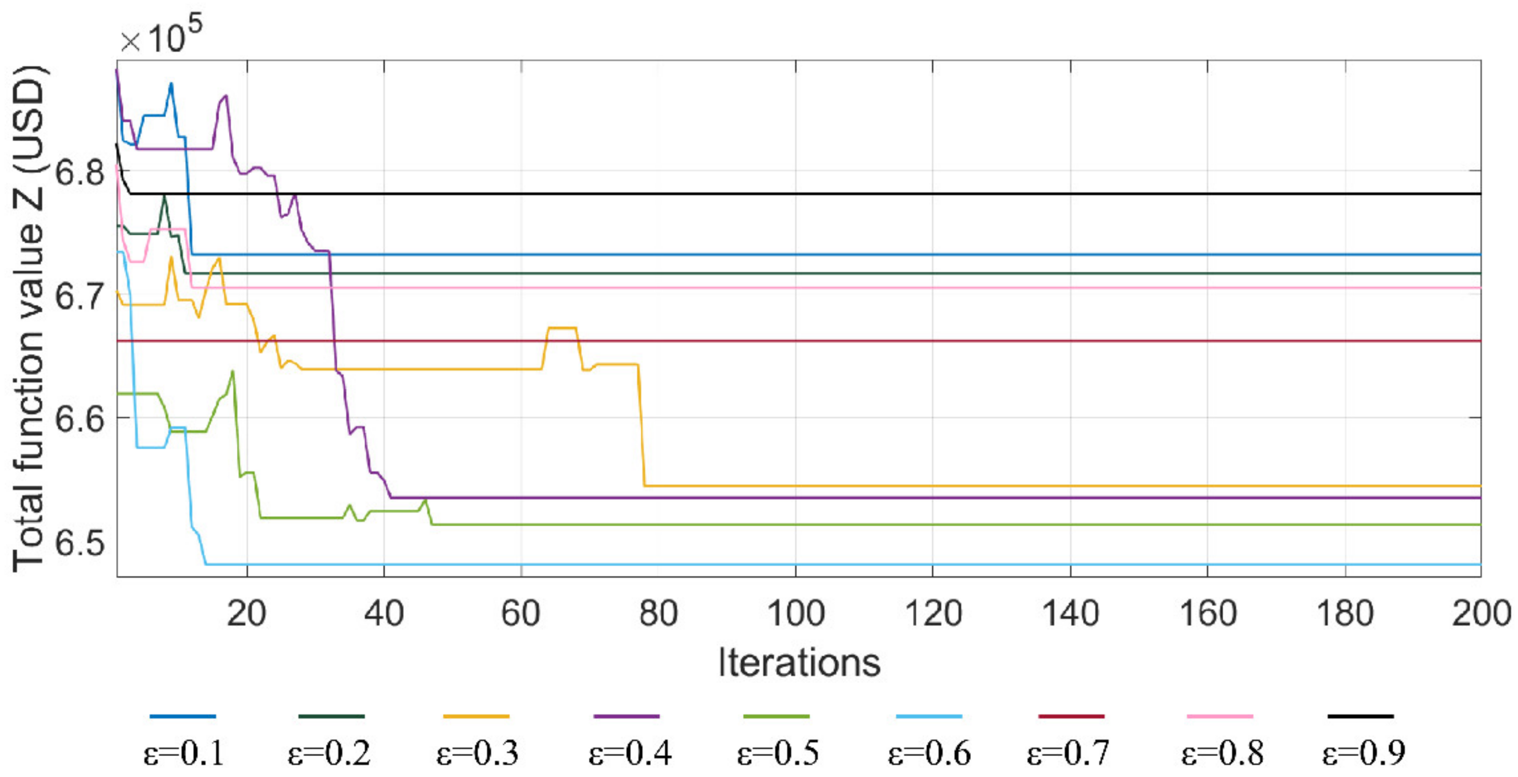
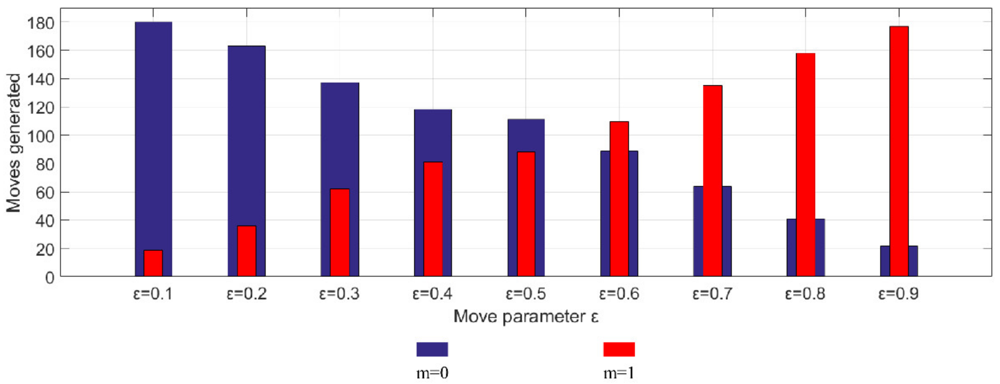
4. Research Results
5. Discussion
6. Conclusions
Author Contributions
Funding
Institutional Review Board Statement
Informed Consent Statement
Acknowledgments
Conflicts of Interest
References
- Michaelis, M.; Schöbel, A. Integrating Line Planning, Timetabling, and Vehicle Scheduling: A Customer-Oriented Heuristic. Public Transp. 2009, 1, 211–232. [Google Scholar] [CrossRef]
- Wang, Y.; Tang, T.; Ning, B.; Meng, L. Integrated optimization of regular train schedule and train circulation plan for urban rail transit lines. Transp. Res. Part E Logist. Transp. Rev. 2017, 105, 83–104. [Google Scholar] [CrossRef]
- Wang, Y.; D’Ariano, A.; Yin, J.; Meng, L.; Tang, T.; Ning, B. Passenger demand oriented train scheduling and rolling stock circulation planning for an urban rail transit line. Transp. Res. Part B Methodol. 2018, 118, 193–227. [Google Scholar] [CrossRef]
- Shi, F.; Zhao, S.; Zhou, Z.; Wang, P.; Bell, M. Optimizing train operational plan in an urban rail corridor based on the maximum headway function. Transp. Res. Part C Emerg. Technol. 2017, 74, 51–80. [Google Scholar] [CrossRef]
- Schöbel, A. Line planning in public transportation: Models and methods. OR Spectr. 2012, 34, 491–510. [Google Scholar] [CrossRef]
- Bussieck, M.R.; Kreuzer, P.; Zimmermann, U.T. Optimal lines for railway systems. Eur. J. Oper. Res. 1997, 96, 54–63. [Google Scholar] [CrossRef]
- Claessens, M.; van Dijk, N.; Zwaneveld, P. Cost optimal allocation of rail passenger lines. Eur. J. Oper. Res. 1998, 110, 474–489. [Google Scholar] [CrossRef]
- Borndörfer, R.; Grötschel, M.; Pfetsch, M. A Column-Generation Approach to Line Planning in Public Transport. Transp. Sci. 2007, 41, 123–132. [Google Scholar] [CrossRef]
- Shi, F.; Deng, L.; Huo, L. Bi-level programming model and algorithm of passenger train operation plan. China Railw. Sci. 2007, 28, 110–116. [Google Scholar]
- Deng, L.; Zeng, Q.; Gao, W.; Zhou, Z. Optimization Method for Train Plan of Urban Rail Transit. In Proceedings of the 11th International Conference of Chinese Transportation Professionals, Nanjing, China, 14–17 August 2011; American Society of Civil Engineers (ASCE): Beijing, China, 2012. [Google Scholar]
- Deng, L.; Zeng, Q.; Gao, W.; Bin, S. Optimization of train plan for urban rail transit in the multi-routing mode. J. Mod. Transp. 2011, 19, 233–239. [Google Scholar] [CrossRef]
- Nachtigall, K.; Voget, S. A genetic algorithm approach to periodic railway synchronization. Comput. Oper. Res. 1996, 23, 453–463. [Google Scholar] [CrossRef]
- Kwan, C.; Chang, C. Application of Evolutionary Algorithm on a Transportation Scheduling Problem-The Mass Rapid Transit. In Proceedings of the IEEE Congress on Evolutionary Computation, Edinburgh, UK, 2–5 September 2005. [Google Scholar]
- Liebchen, C. Periodic Timetable Optimization in Public Transport. In Operations Research Proceedings; Springer: Berlin/Heidelberg, Germany, 2006. [Google Scholar]
- Albrecht, T. Automated timetable design for demand-oriented service on suburban railways. Public Transp. 2008, 1, 5–20. [Google Scholar] [CrossRef]
- Su, S.; Li, X.; Tang, T.; Gao, Z. A Subway Train Timetable Optimization Approach Based on Energy-Efficient Operation Strategy. IEEE Trans. Intell. Transp. Syst. 2013, 14, 883–893. [Google Scholar] [CrossRef]
- Sun, L.; Jin, J.G.; Lee, D.-H.; Axhausen, K.W.; Erath, A. Demand-driven timetable design for metro services. Transp. Res. Part C Emerg. Technol. 2014, 46, 284–299. [Google Scholar] [CrossRef]
- Wang, Y.; Tang, T.; Ning, B.; Boom, T.J.V.D.; De Schutter, B. Passenger-demands-oriented train scheduling for an urban rail transit network. Transp. Res. Part C Emerg. Technol. 2015, 60, 1–23. [Google Scholar] [CrossRef]
- Abbink, E.; Berg, B.V.D.; Kroon, L.; Salomon, M. Allocation of Railway Rolling Stock for Passenger Trains. Transp. Sci. 2004, 38, 33–41. [Google Scholar] [CrossRef]
- Fioole, P.-J.; Kroon, L.; Maroti, G.; Schrijver, A. A rolling stock circulation model for combining and splitting of passenger trains. Eur. J. Oper. Res. 2006, 174, 1281–1297. [Google Scholar] [CrossRef]
- Alfieri, A.; Groot, R.; Kroon, L.; Schrijver, A. Efficient Circulation of Railway Rolling Stock. Transp. Sci. 2006, 40, 378–391. [Google Scholar] [CrossRef]
- Withall, M.S.; Hinde, C.; Jackson, T.; Phillips, I.; Brown, S.; Watson, R. Automating Rolling Stock Diagramming and Platform Allocation. In Proceedings of the 9th World Congress on Railway Research, World Congress on Railway Research (WCRR) © SNCF, Lille, France, 22–26 May 2011. [Google Scholar]
- Blanco, V.; Conde, E.; Hinojosa, Y.; Puerto, J. An optimization model for line planning and timetabling in automated urban metro subway networks. A case study. Omega 2019, 92, 102165. [Google Scholar] [CrossRef]
- Zhou, W.; Shi, F.; Chen, Y.; Deng, L. Method of integrated optimization of train operation plan and diagram for network of dedicated passenger lines. J. China Railw. Soc. 2011, 1–7. [Google Scholar]
- Zhou, W.; Tian, J.; Deng, L.; Qin, J. Integrated Optimization of Service-Oriented Train Plan and Schedule on Intercity Rail Network with Varying Demand. Discret. Dyn. Nat. Soc. 2015, 2015, 1–9. [Google Scholar] [CrossRef]
- Burggraeve, S.; Bull, S.H.; Vansteenwegen, P.; Lusby, R.M. Integrating robust timetabling in line plan optimization for railway systems. Transp. Res. Part C Emerg. Technol. 2017, 77, 134–160. [Google Scholar] [CrossRef]
- Shen, Y.; Xie, W.; Li, J. A MultiObjective Optimization Approach for Integrated Timetabling and Vehicle Scheduling with Uncertainty. J. Adv. Transp. 2021, 2021, 1–16. [Google Scholar] [CrossRef]
- Petersen, H.L.; Larsen, A.; Madsen, O.B.G.; Petersen, B.; Ropke, S. The Simultaneous Vehicle Scheduling and Passenger Service Problem. Transp. Sci. 2013, 47, 603–616. [Google Scholar] [CrossRef]
- Su, H.; Tao, W.; Hu, X. A Line Planning Approach for High-Speed Rail Networks with Time-Dependent Demand and Capacity Constraints. Math. Probl. Eng. 2019, 2019, 1–18. [Google Scholar] [CrossRef]
- Heidari, M.; Hosseini-Motlagh, S.M.; Nikoo, N. A subway planning bi-objective multi-period optimization model integrating timetabling and vehicle scheduling: A case study of Tehran. Transportation 2020, 47, 417–443. [Google Scholar] [CrossRef]
- Yue, Y.; Han, J.; Wang, S.; Liu, X. Integrated Train Timetabling and Rolling Stock Scheduling Model Based on Time-Dependent Demand for Urban Rail Transit. Comput. Civ. Infrastruct. Eng. 2017, 32, 856–873. [Google Scholar] [CrossRef]
- Ibarra-Rojas, O.J.; Giesen, R.; Rios-Solis, Y. An integrated approach for timetabling and vehicle scheduling problems to analyze the trade-off between level of service and operating costs of transit networks. Transp. Res. Part B Methodol. 2014, 70, 35–46. [Google Scholar] [CrossRef]
- Li, W.; Yan, X.; Li, X.; Yang, J. Estimate Passengers’ Walking and Waiting Time in Metro Station Using Smart Card Data (SCD). IEEE Access 2020, 8, 11074–11083. [Google Scholar] [CrossRef]
- Zhang, S.; Dong, H.; Zhu, H. Optimal Train Schedule With Headway And passenger Flow Dynamic Models. In Proceedings of the IEEE International Conference on Intelligent Rail Transportation (ICIRT), Beijing, China, 30 August 2013. [Google Scholar]


| Study | Sub- Problems | Factors Considered | Objectives | Solution Method |
|---|---|---|---|---|
| [15] | T 2 | H 4, RSC 5 | Minimizing enterprise operating costs | Branch-and-bound and genetic algorithm |
| [4] | LP 1, T 2, RSA 3 | PC 6 | Maximum headway function, Minimization of depot circulations and number of rolling stock used | Linear computation |
| [4] | LP 1 | TC 5 | Minimizing enterprise operating cost & passengers travel cost | Three phase solving algorithm |
| [11] | LP 1 | RSC 5, PBC 8 | Minimizing enterprise operating cost & passengers travel cost | Three phase solving algorithm |
| [2] | T 2, RSA 3 | NRS 7, CD 9, TO 10 | Minimize headway variation, minimize number of rolling stock, minimize passengers waiting time | Transforming the model to MILP 13 problem and solving with CPLEX |
| [3] | T 2, RSA 3 | RSC 5, NRS 7, CD 9 | Passenger oriented multi-objective function | Iterative nonlinear programming. Accurate/approximated MILP 13 |
| [17] | T 2 | RSC 5 | Minimizing waiting time | CPLEX solver |
| (This study) | LP 1, T 2, RSA 3 | PFA 12, DW 11, H 4 | Minimizing enterprise operation costs and passenger travelling costs | Simulated annealing-based algorithm |
| Variables | Definitions |
|---|---|
| 0–1 binary decision variable, it shows whether or not candidate trip is chosen for up-direction operation, if yes, then , otherwise, . | |
| 0–1 binary decision variable, it indicates whether or not candidate trip of down-direction is chosen to operate, if yes, then , otherwise, . | |
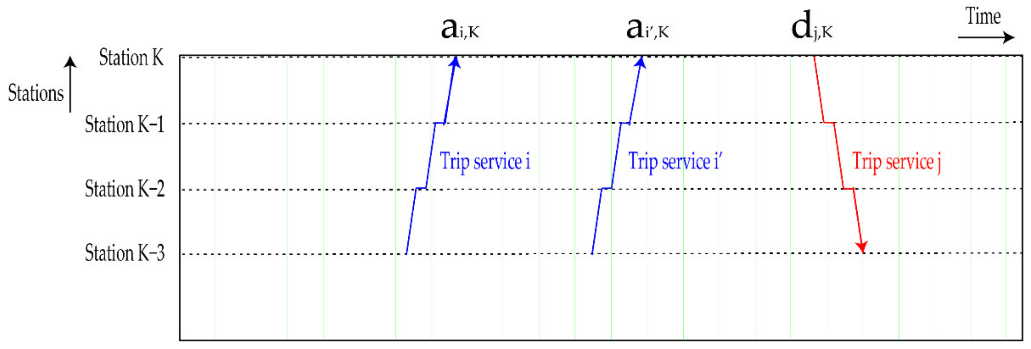
| Departure time of up-direction trip from station | |
| Arrival time of up-direction trip to station | |
| Departure time of down-direction trip from station | |
| Arrival time of down-direction trip to station | |
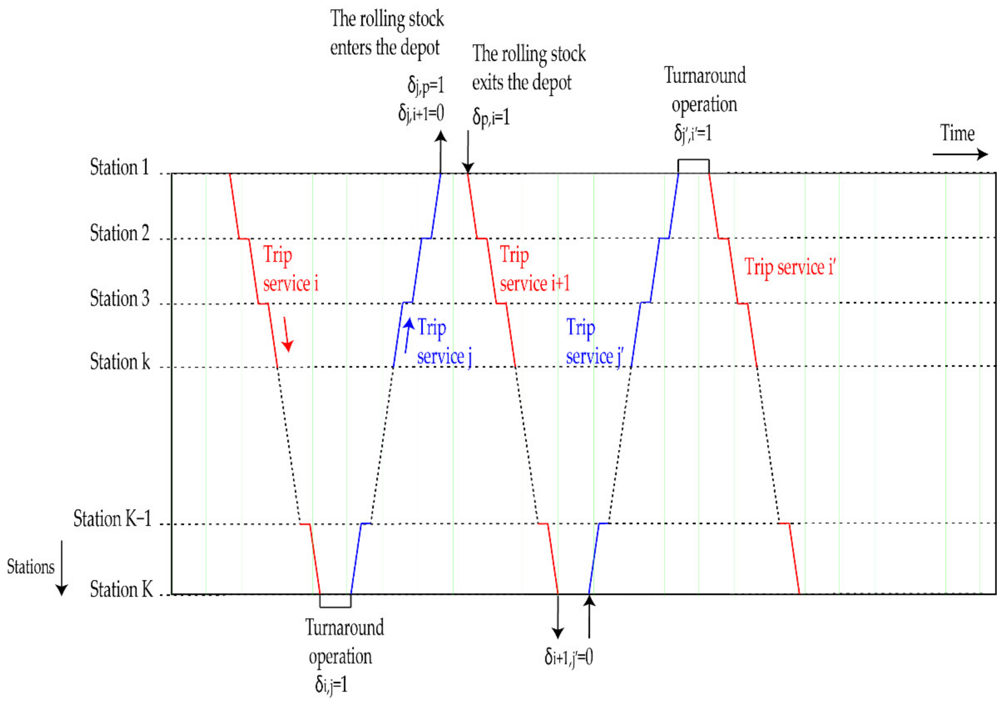
| 0–1 binary decision variable, it shows whether or not the rolling stock allocated for service comes from the depot, if yes, then , otherwise, . | |
| 0–1 binary decision variable, it shows whether or not the rolling stock enters the depot after servicing trip , if yes, then , otherwise, . | |
| 0–1 binary decision variable, it shows whether or not a rolling stock continues to service trip after servicing trip at station 1, if yes, then , otherwise, . | |
| 0–1 binary decision variable, it shows whether or not a rolling stock continues to service trip after servicing at station , if yes, then , otherwise, . |
| Notations | Definitions |
|---|---|
| The start and end of the day operation | |
| The start and end of operation period | |
| Indexes for trip services | |
| Sets of upstream trip services | |
| Set of upstream trip services during operation period | |
| Sets of downstream trip services | |
| Set of downstream trip services during operation period | |
| Indexes used for stations | |
| Index for time periods | |
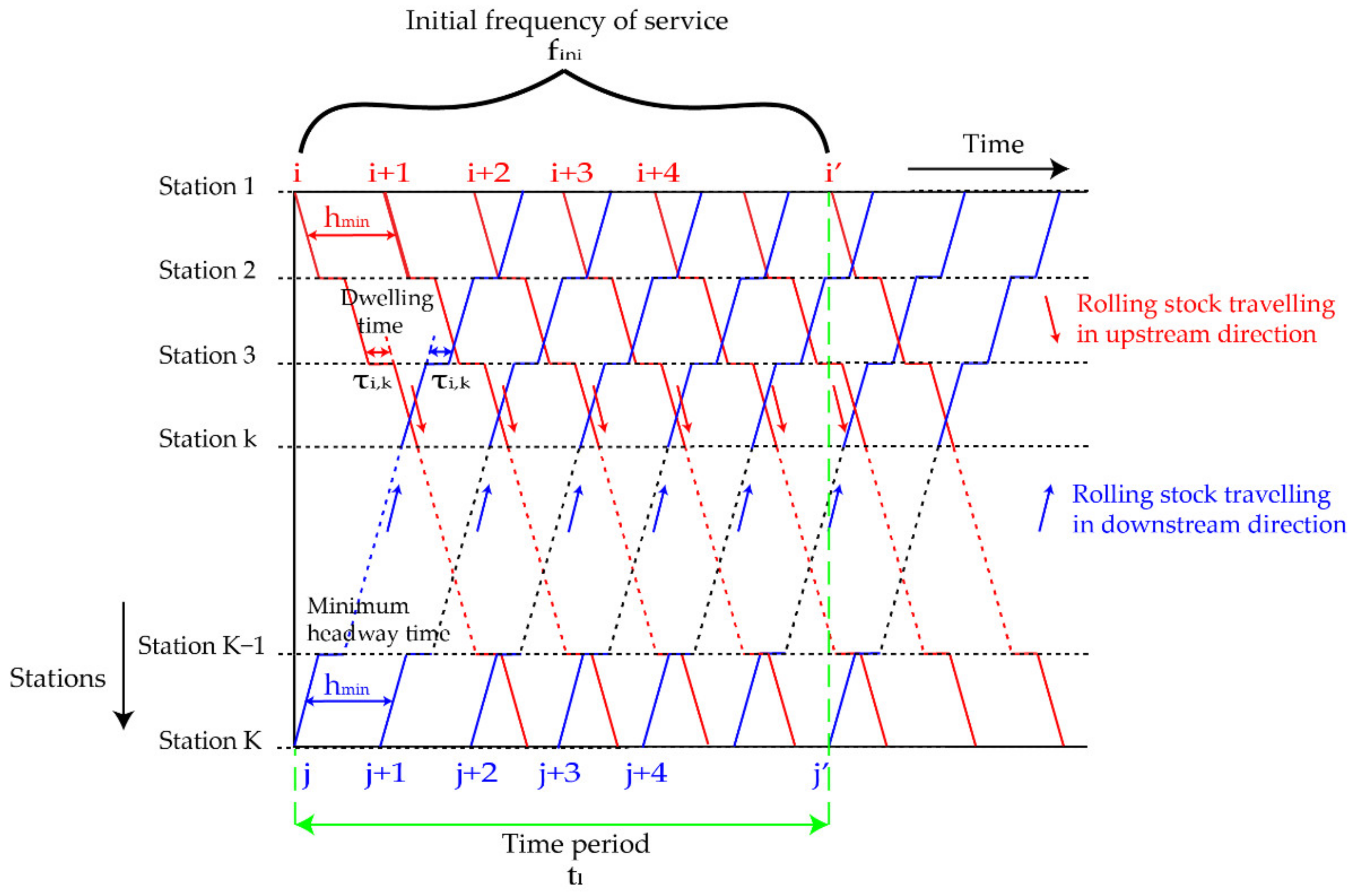
| Initial service frequency based on minimum headway | |
| Arriving time of the passenger to the station | |
| Total capacity of the rolling stock | |
| Fare rate | |
| Weight factor | |
| Average time value of passengers | |
| Cost per time unit of service | |
| Penalty related to late arriving passengers | |
| Minimum running time of trip service from station to the next station | |
| Minimum running time of trip service from station to the next station | |
| Minimum time required for a turnaround operation at terminal stations | |
| Time required for rolling stock to enter the depot | |
| Time required for rolling stock to exit the depot | |
| Headway time representing the time difference between two consecutive servicing trips | |
| Minimum headway time value | |
| Maximum headway time value | |
| Minimum dwell time of servicing trip at station | |
| Minimum dwell time of servicing trip at station | |
| Average time required for the boarding and alighting of a passenger | |
| Reaction time of a passenger to boarding and alighting operation |
| Notations | Definitions |
| Time limit for passengers to board the rolling stock before it reaches its max capacity | |
| Dividing time deciding whether passengers arrive in time to board the rolling stock | |
| Boarding capacity of the rolling stock servicing trip when arriving to station | |
| Boarding capacity of the rolling stock servicing trip when arriving to station | |
| Number of passengers boarding the rolling stock servicing trip travelling to station | |
| Number of passengers boarding the rolling stock servicing trip travelling to station | |
| Number of passengers boarding the rolling stock servicing up-direction trip at station | |
| Number of passengers boarding the rolling stock servicing down-direction trip at station | |
| Number of passengers alighting from the rolling stock servicing up-direction trip at station | |
| Number of passengers alighting from the rolling stock servicing down-direction trip at station |
| Notations | Definitions |
|---|---|
| Passengers’ arrival rate at station travelling to station at time |
| Parameters | Values | Parameters | Values |
|---|---|---|---|
| Scheduled Trips | Circulation to/from the Depot | ||||
|---|---|---|---|---|---|
Publisher’s Note: MDPI stays neutral with regard to jurisdictional claims in published maps and institutional affiliations. |
© 2021 by the authors. Licensee MDPI, Basel, Switzerland. This article is an open access article distributed under the terms and conditions of the Creative Commons Attribution (CC BY) license (https://creativecommons.org/licenses/by/4.0/).
Share and Cite
Zhou, W.; Oldache, M. Integrated Optimization of Line Planning, Timetabling and Rolling Stock Allocation for Urban Railway Lines. Sustainability 2021, 13, 13059. https://doi.org/10.3390/su132313059
Zhou W, Oldache M. Integrated Optimization of Line Planning, Timetabling and Rolling Stock Allocation for Urban Railway Lines. Sustainability. 2021; 13(23):13059. https://doi.org/10.3390/su132313059
Chicago/Turabian StyleZhou, Wenliang, and Mehdi Oldache. 2021. "Integrated Optimization of Line Planning, Timetabling and Rolling Stock Allocation for Urban Railway Lines" Sustainability 13, no. 23: 13059. https://doi.org/10.3390/su132313059
APA StyleZhou, W., & Oldache, M. (2021). Integrated Optimization of Line Planning, Timetabling and Rolling Stock Allocation for Urban Railway Lines. Sustainability, 13(23), 13059. https://doi.org/10.3390/su132313059