Author Contributions
Conceptualization, A.R., S.K. and M.H.H.; data curation, M.T.-V. and A.M.E.; formal analysis, A.R., S.K. and M.H.H.; funding acquisition, M.T.-V., S.K. and A.M.E.; investigation, A.R., S.K. and M.H.H.; methodology, A.R., S.K. and M.H.H.; project administration, M.T.-V. and A.M.E.; resources, M.T.-V. and A.M.E.; software, A.R., M.H.H. and S.K.; supervision, S.K., M.T.-V., and A.M.E.; validation, A.R., S.K. and M.H.H.; visualization, M.T.-V. and A.M.E.; writing—original draft, A.R., S.K. and M.H.H.; writing—review and editing, M.T.-V. and A.M.E. All authors have read and agreed to the published version of the manuscript.
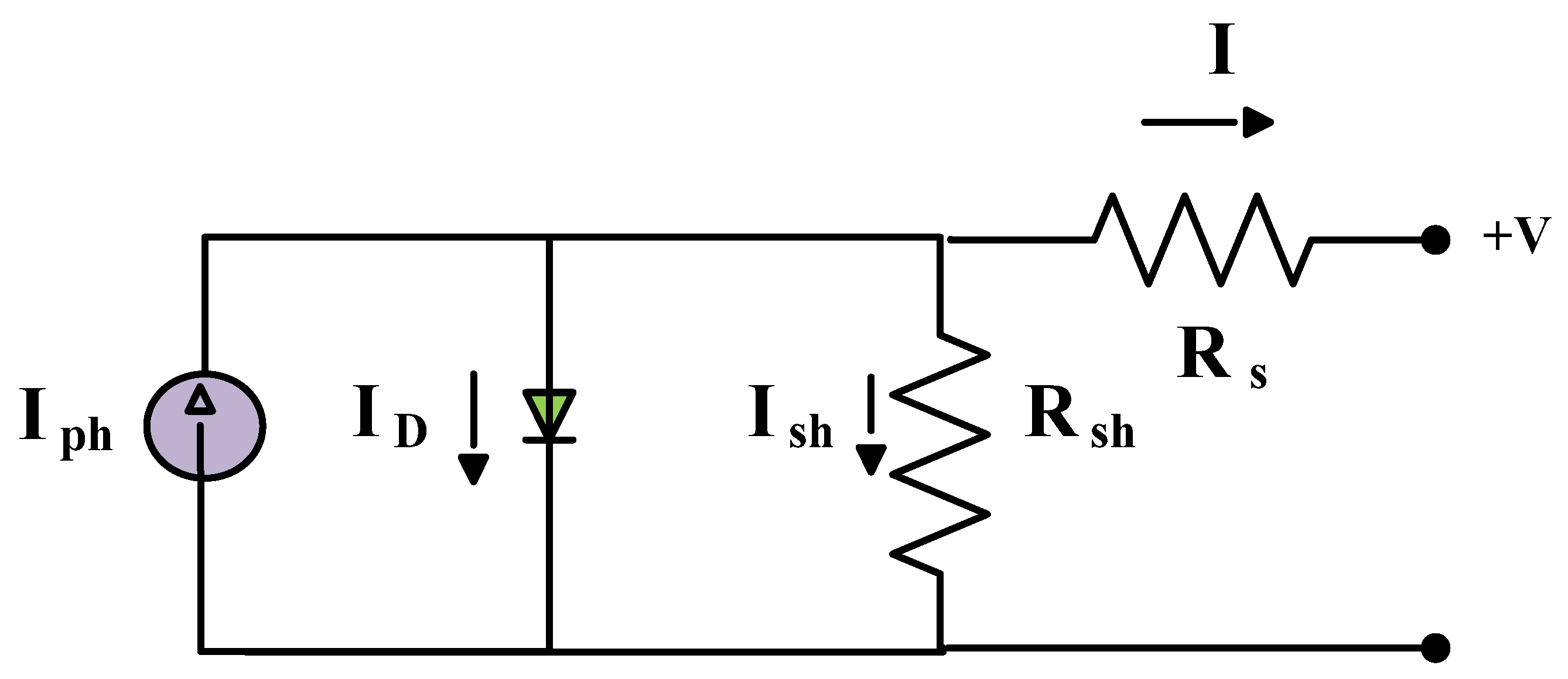
Figure 3.
Integral Order Dynamic Model.
Figure 3.
Integral Order Dynamic Model.
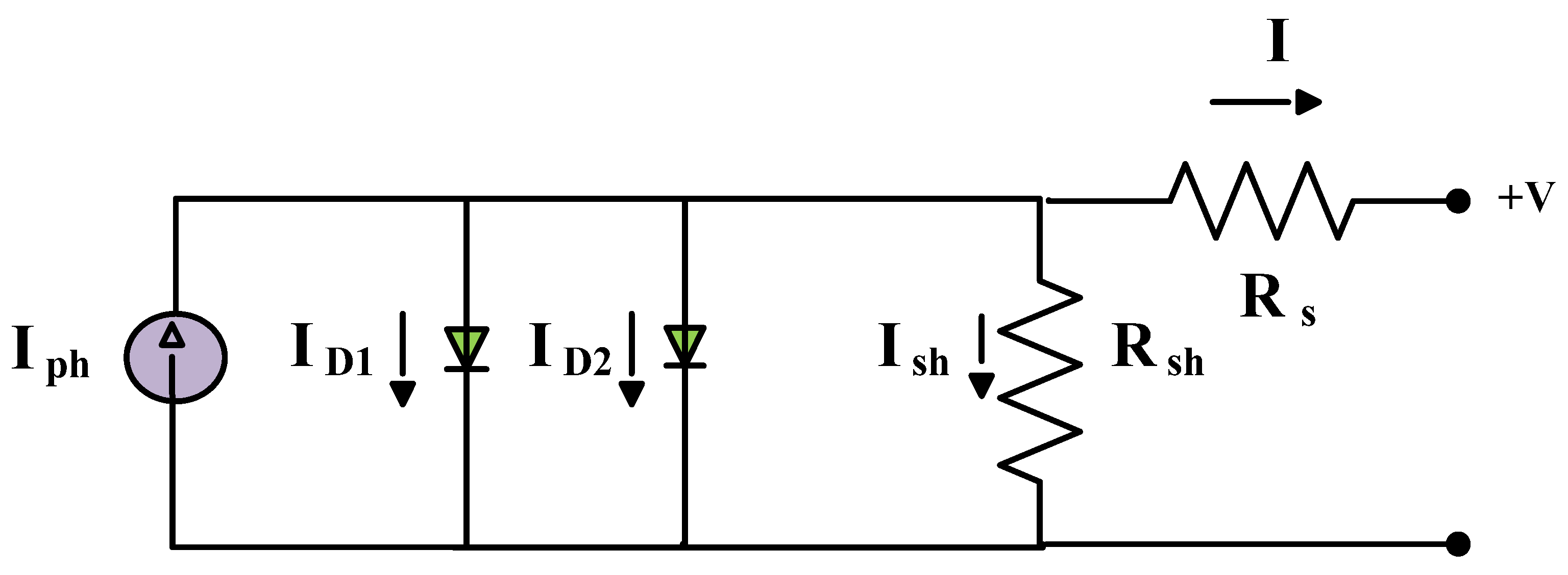
Figure 4.
Fractional Order dynamic model.
Figure 4.
Fractional Order dynamic model.
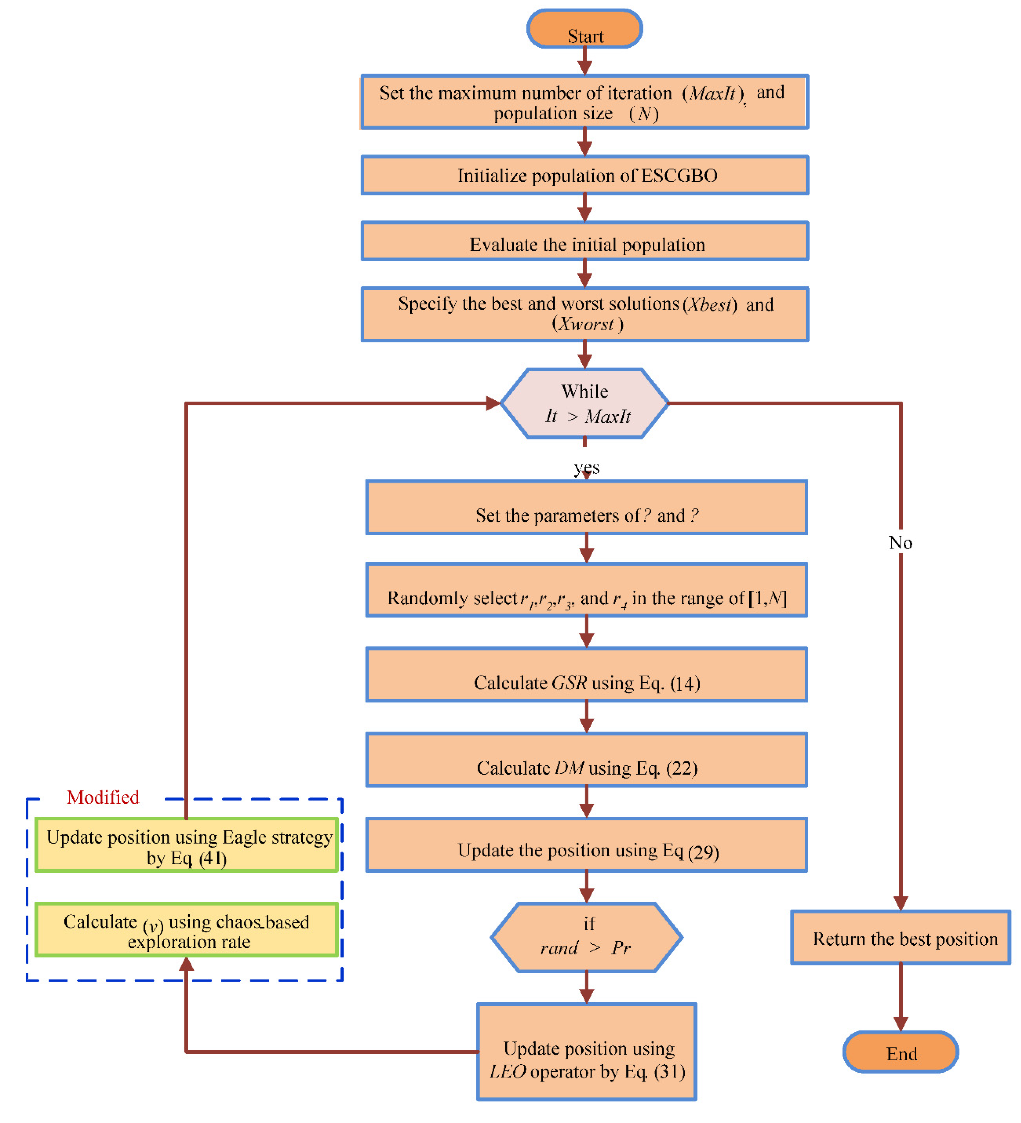
Figure 5.
Flowchart of the proposed ESCGBO algorithm.
Figure 5.
Flowchart of the proposed ESCGBO algorithm.
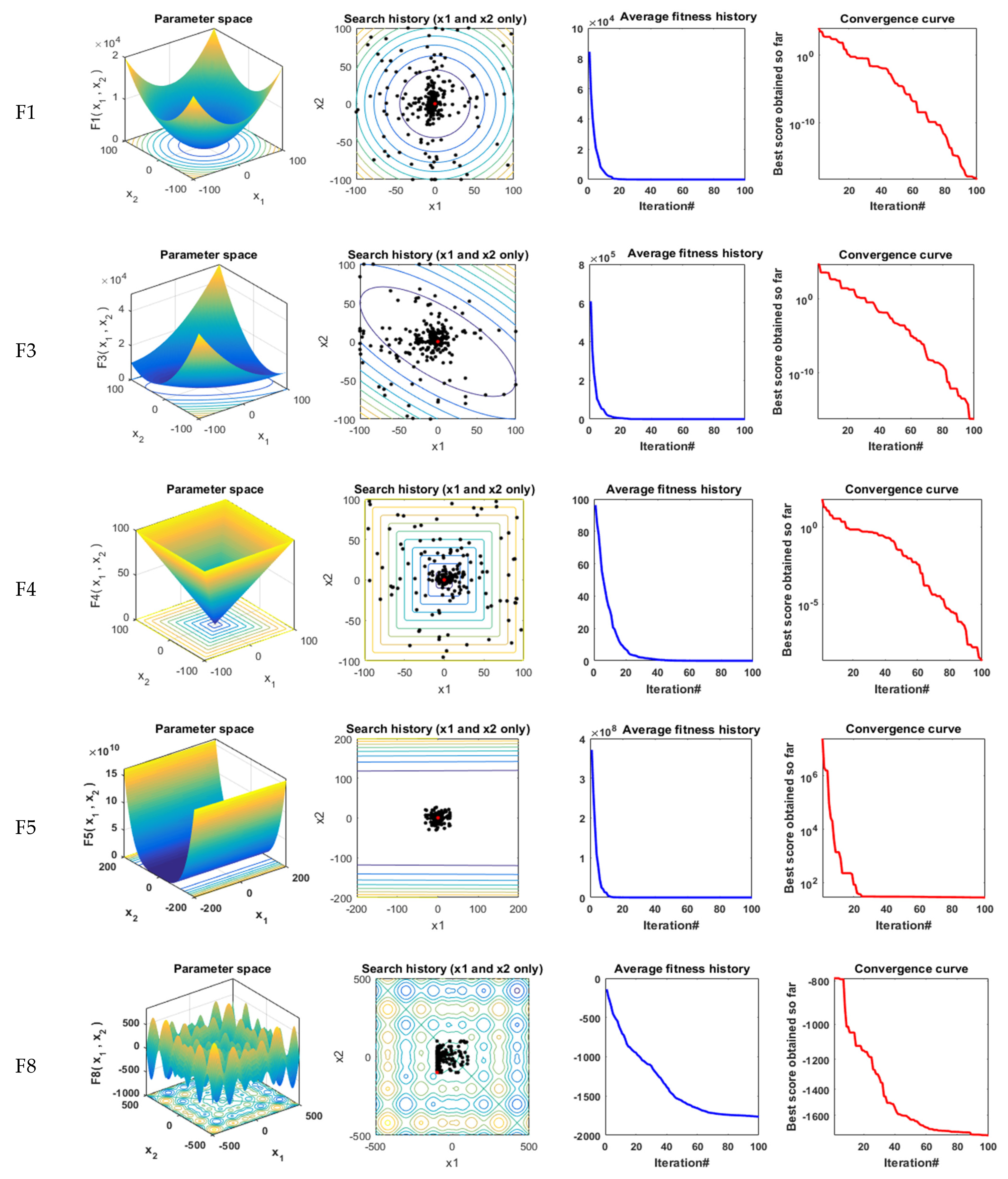
Figure 6.
Qualitative metrics on F1, F3, F4, F5, F8, F12, F15, and F18: 2D views of the functions, search history, average fitness history, and convergence curve using ESCGBO algorithm.
Figure 6.
Qualitative metrics on F1, F3, F4, F5, F8, F12, F15, and F18: 2D views of the functions, search history, average fitness history, and convergence curve using ESCGBO algorithm.
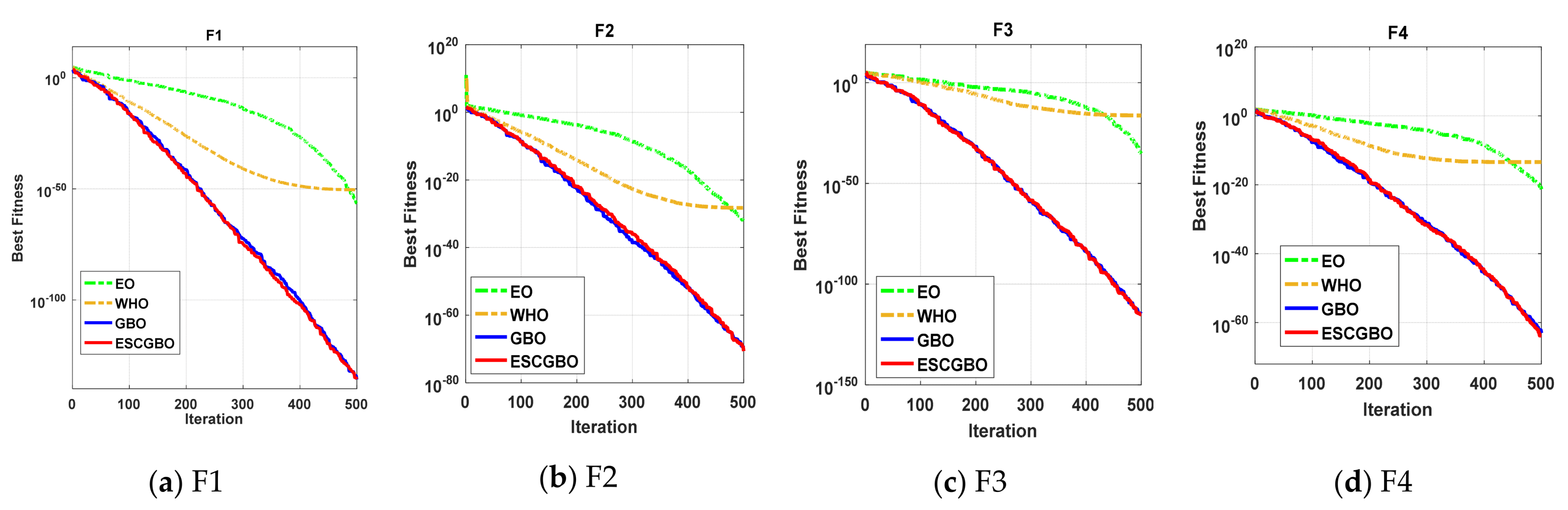
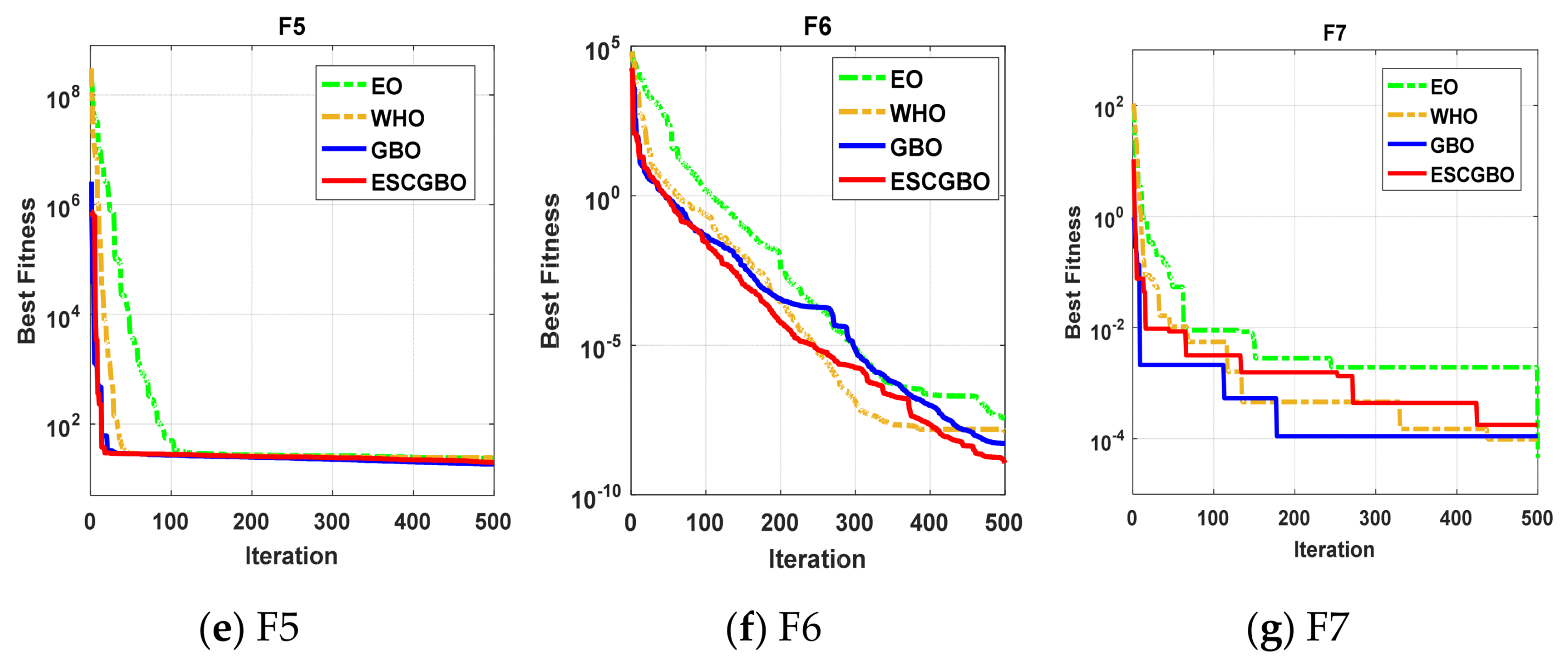
Figure 7.
The convergence curves of all algorithms for unimodal benchmark functions (a) F1, (b) F2, (c) F3, (d) F4, (e) F5, (f) F6, and (g) F7.
Figure 7.
The convergence curves of all algorithms for unimodal benchmark functions (a) F1, (b) F2, (c) F3, (d) F4, (e) F5, (f) F6, and (g) F7.
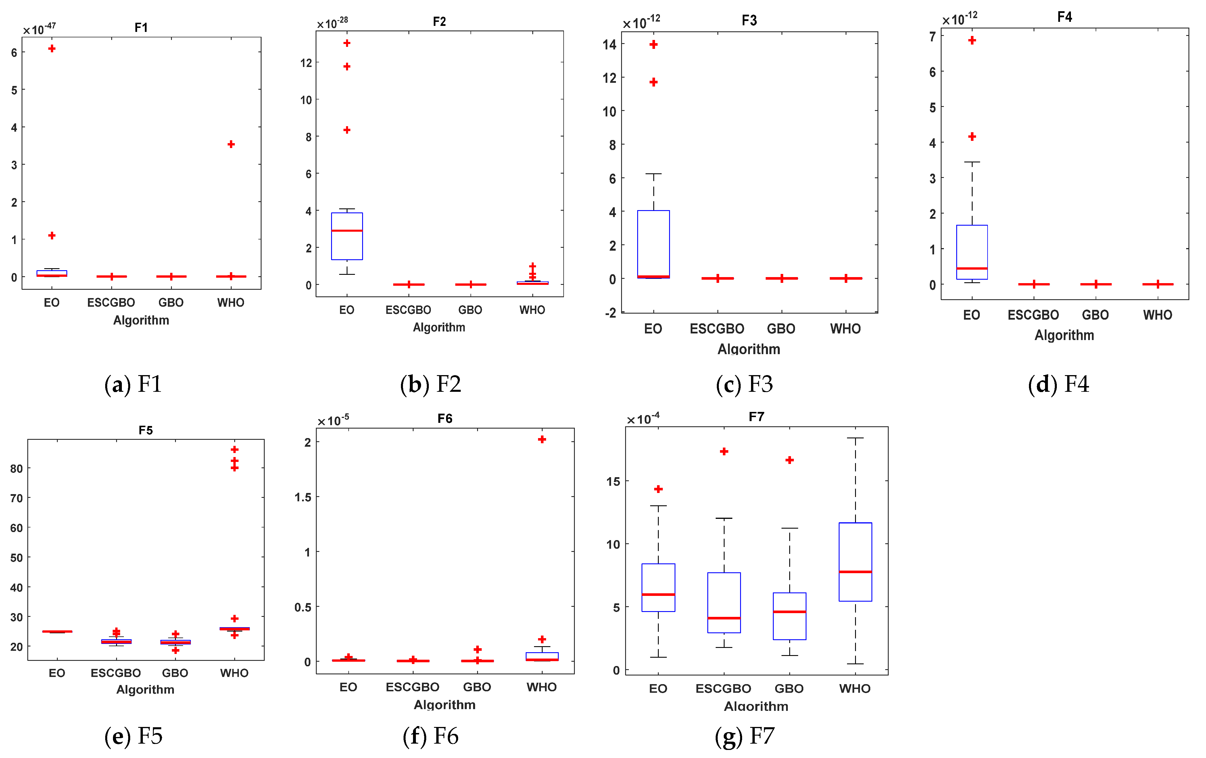
Figure 8.
Boxplots for all algorithms for unimodal benchmark functions (a) F1, (b) F2, (c) F3, (d) F4, (e) F5, (f) F6, and (g) F7.
Figure 8.
Boxplots for all algorithms for unimodal benchmark functions (a) F1, (b) F2, (c) F3, (d) F4, (e) F5, (f) F6, and (g) F7.
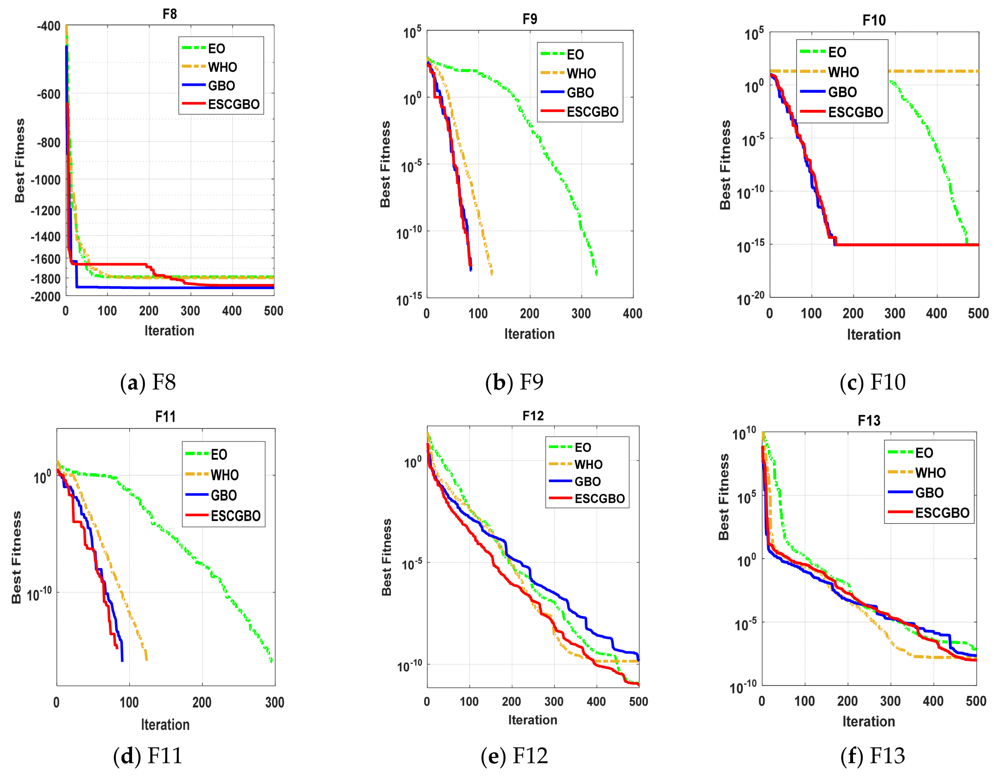
Figure 9.
The convergence curves of all algorithms for multi-modal benchmark functions (a) F8, (b) F9, (c) F10, (d) F11, (e) F12, and (f) F13.
Figure 9.
The convergence curves of all algorithms for multi-modal benchmark functions (a) F8, (b) F9, (c) F10, (d) F11, (e) F12, and (f) F13.
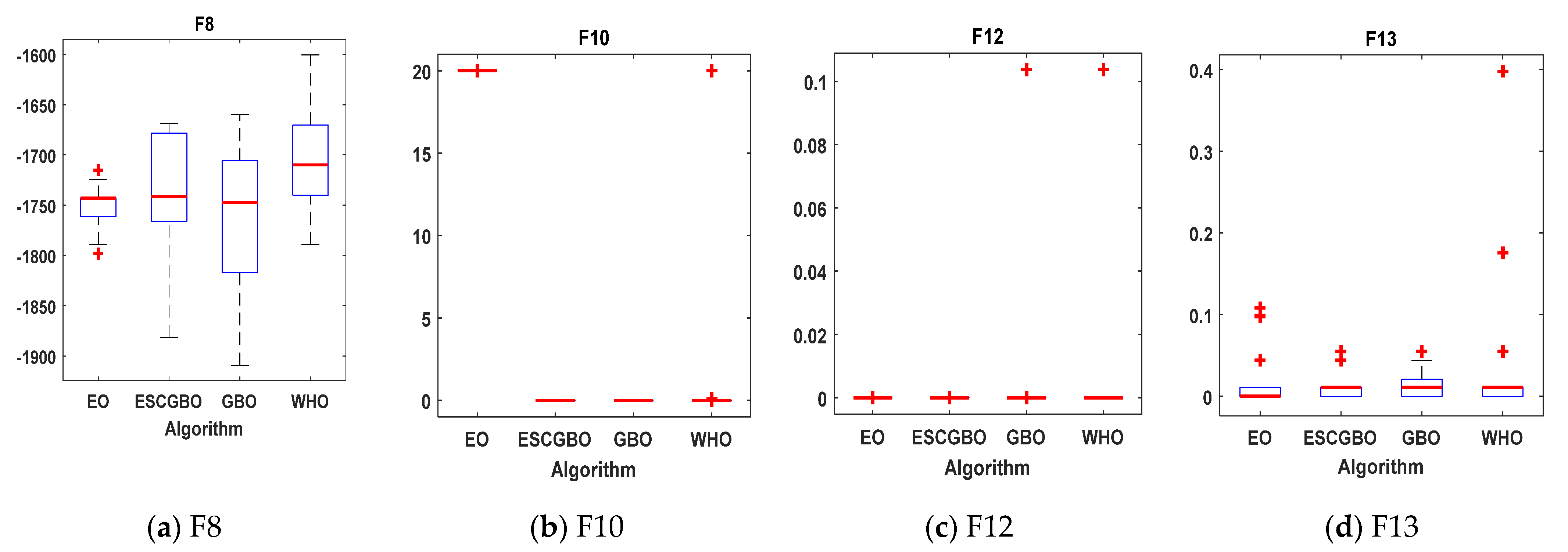
Figure 10.
Boxplots for all algorithms for some of multi-modal benchmark functions (a) F8, (b) F10, (c) F12, and (d) F13.
Figure 10.
Boxplots for all algorithms for some of multi-modal benchmark functions (a) F8, (b) F10, (c) F12, and (d) F13.
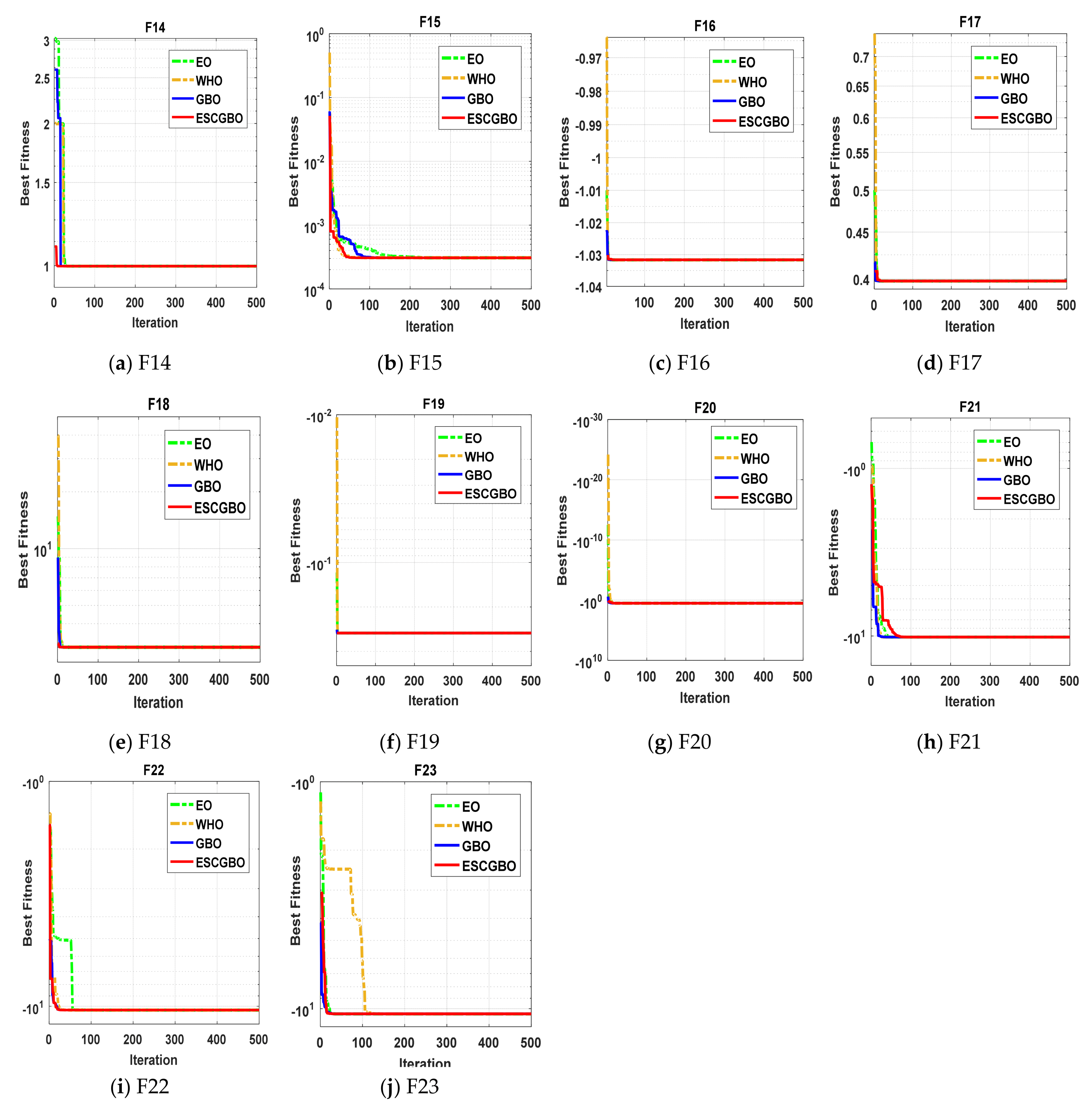
Figure 11.
The convergence curves of all algorithms for composite benchmark functions (a) F14, (b) F15, (c) F16, (d) F17, (e) F18, (f) F19, (g) F20, (h) F21, (i) F22, and (j) F23.
Figure 11.
The convergence curves of all algorithms for composite benchmark functions (a) F14, (b) F15, (c) F16, (d) F17, (e) F18, (f) F19, (g) F20, (h) F21, (i) F22, and (j) F23.
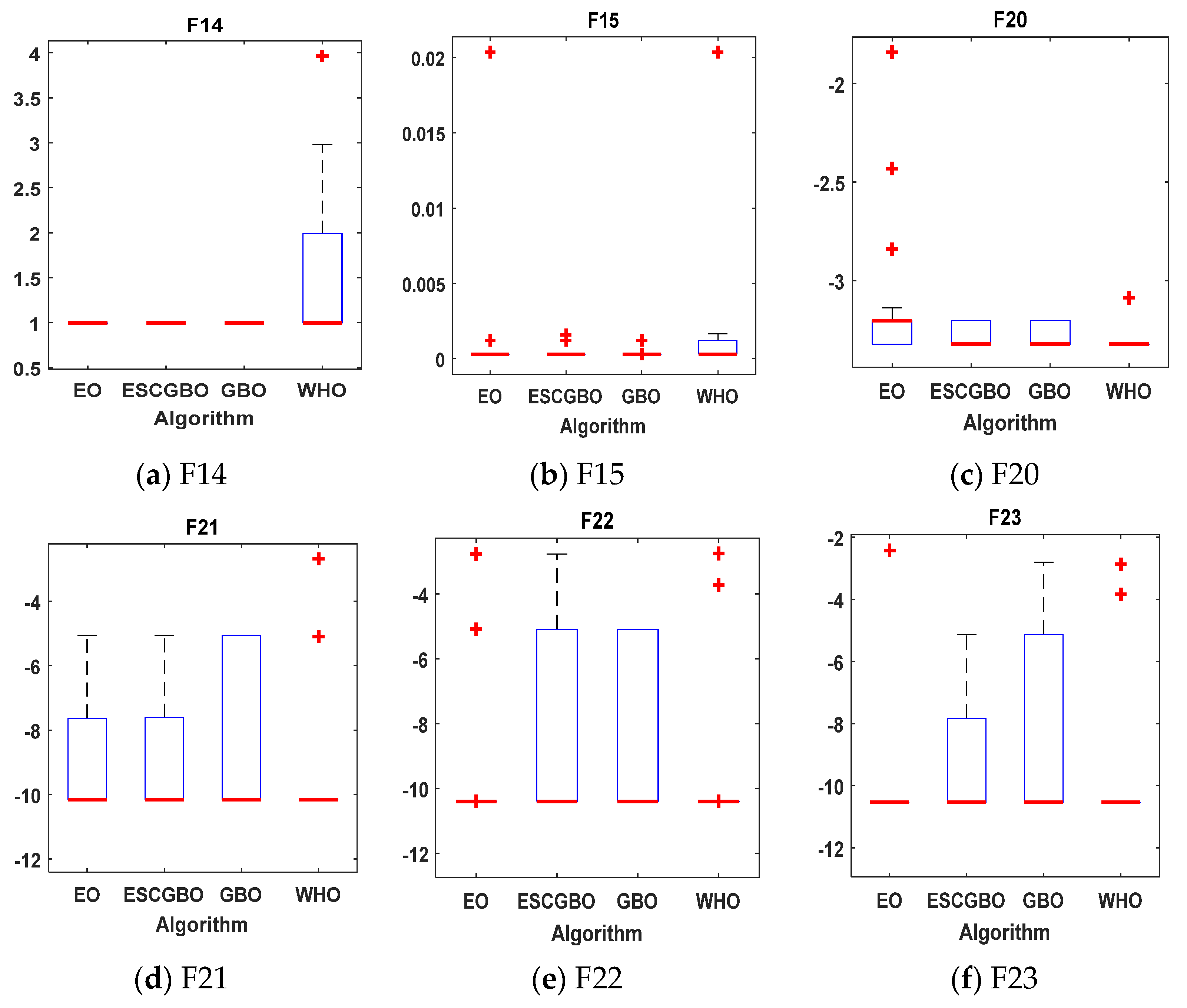
Figure 12.
Boxplots for all algorithms for some of composite benchmark functions (a) F14, (b) F15, (c) F20, (d) F21, (e) F22, and (f) F23.
Figure 12.
Boxplots for all algorithms for some of composite benchmark functions (a) F14, (b) F15, (c) F20, (d) F21, (e) F22, and (f) F23.
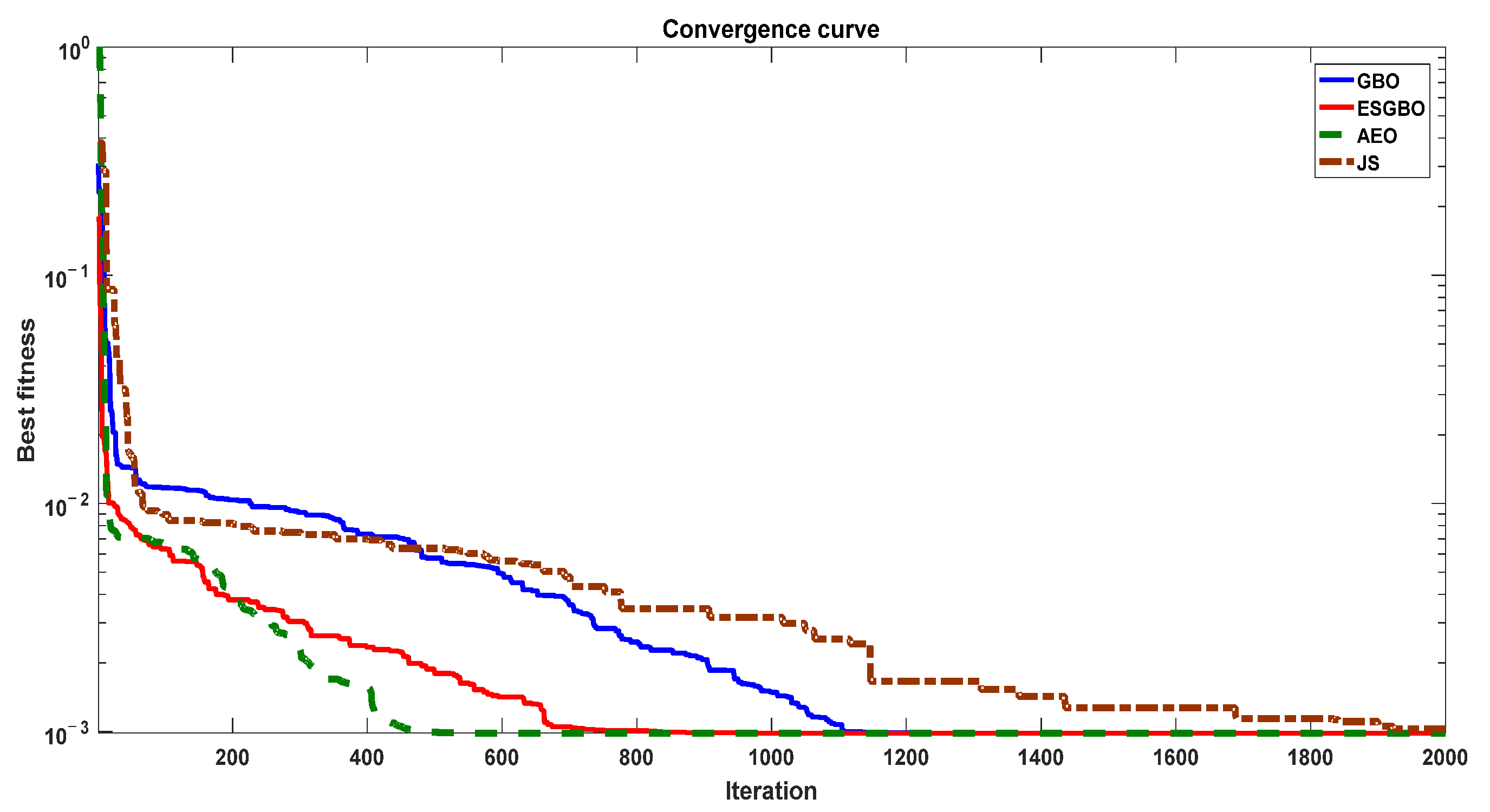
Figure 13.
The convergence curve of all algorithms of SDM.
Figure 13.
The convergence curve of all algorithms of SDM.
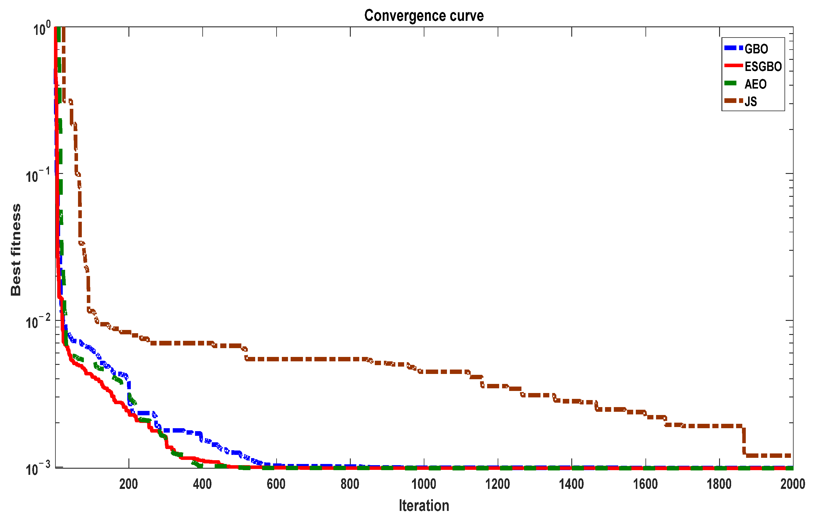
Figure 14.
The convergence curve of all algorithms of DDM.
Figure 14.
The convergence curve of all algorithms of DDM.
Figure 15.
Boxplot figure of all algorithms for 30 independent runs in case of SDM and DDM.
Figure 15.
Boxplot figure of all algorithms for 30 independent runs in case of SDM and DDM.
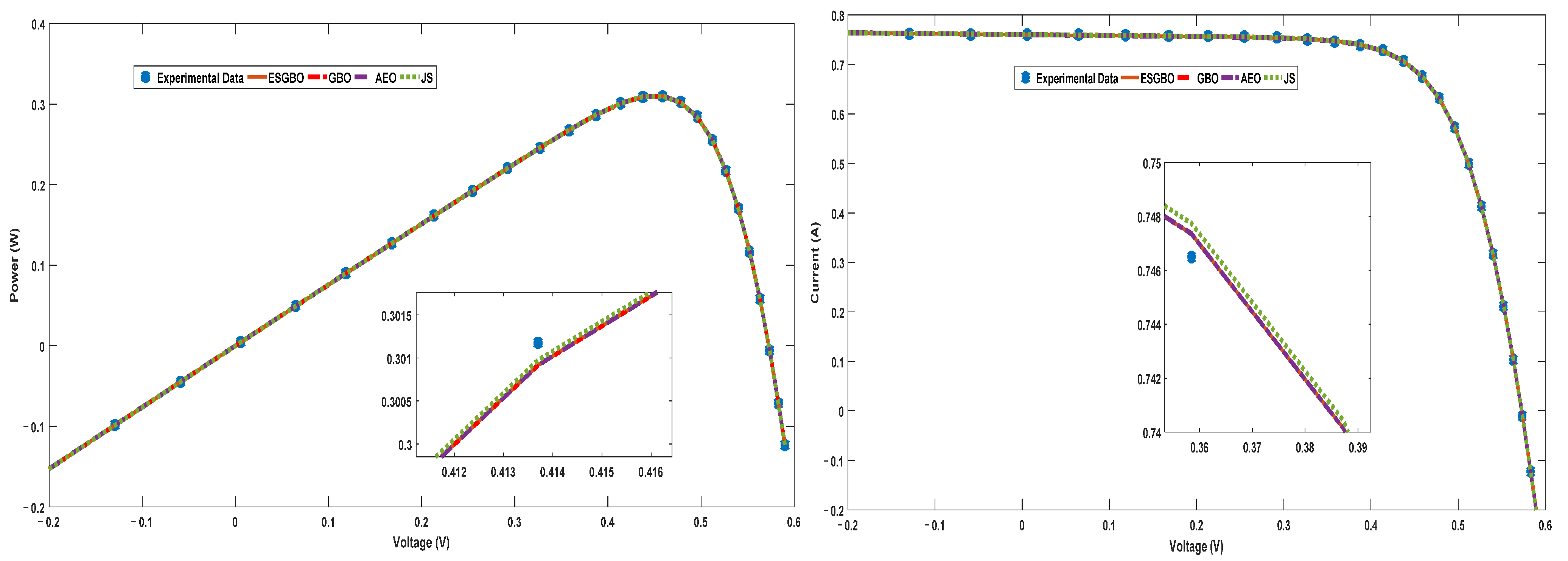
Figure 16.
Power and current characteristics for SDM estimated by all algorithms.
Figure 16.
Power and current characteristics for SDM estimated by all algorithms.
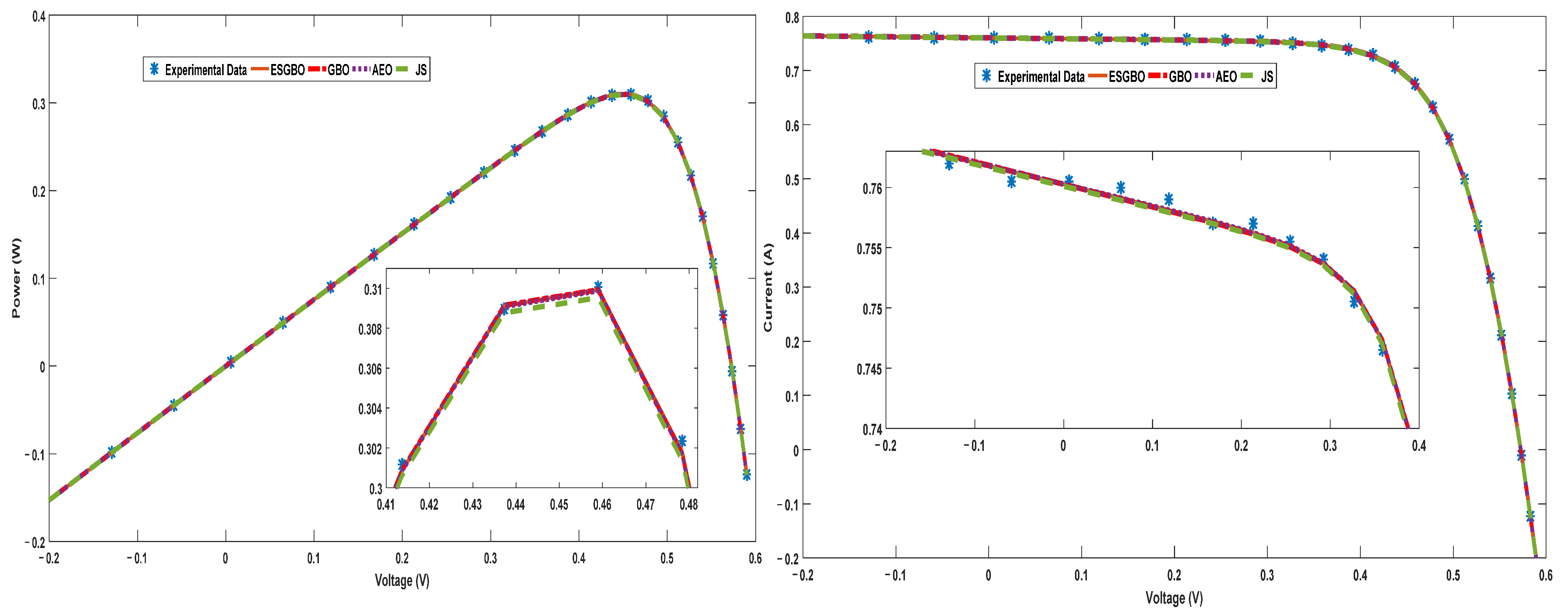
Figure 17.
Power and current characteristics for DDM estimated by all algorithms.
Figure 17.
Power and current characteristics for DDM estimated by all algorithms.
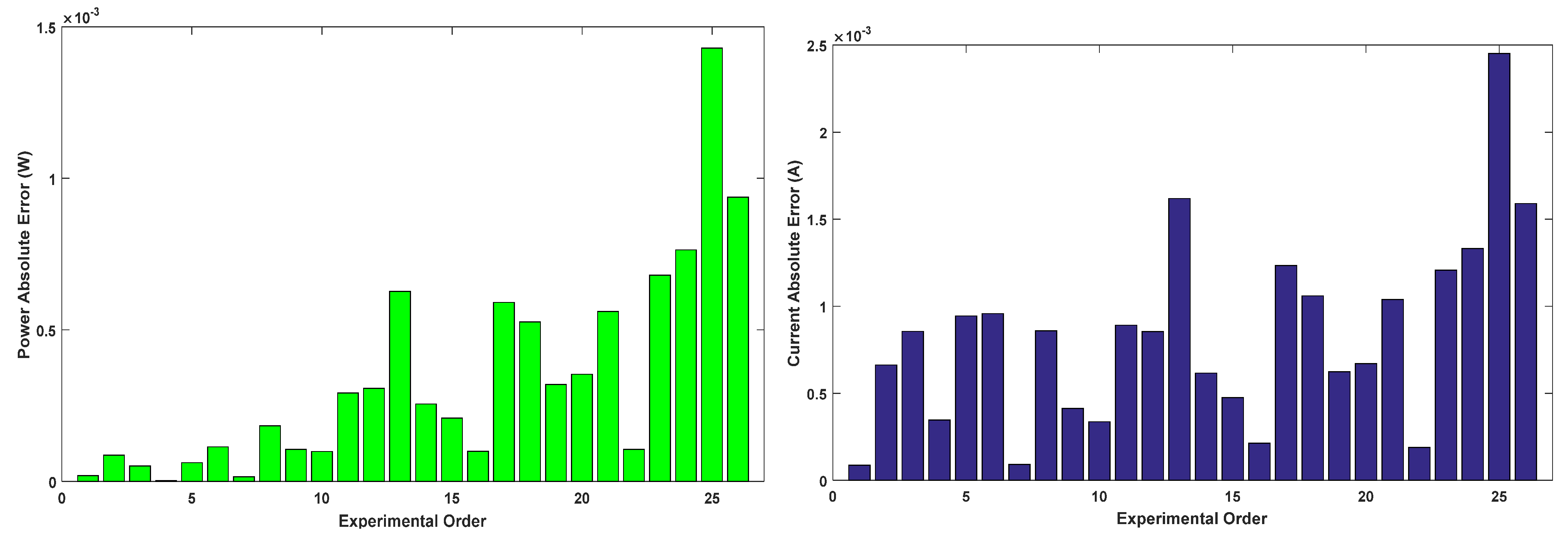
Figure 18.
Power and current absolute error for SDM estimated by all algorithms.
Figure 18.
Power and current absolute error for SDM estimated by all algorithms.
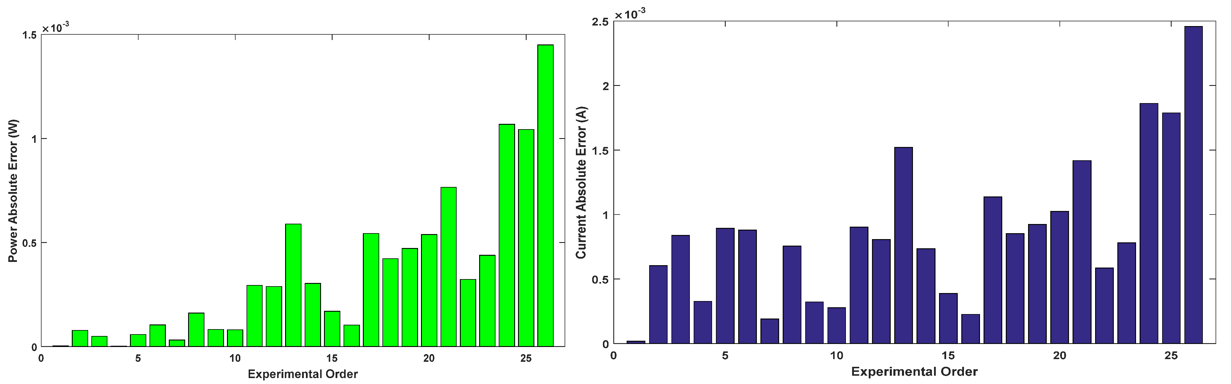
Figure 19.
Power and current absolute error for DDM estimated by all algorithms.
Figure 19.
Power and current absolute error for DDM estimated by all algorithms.
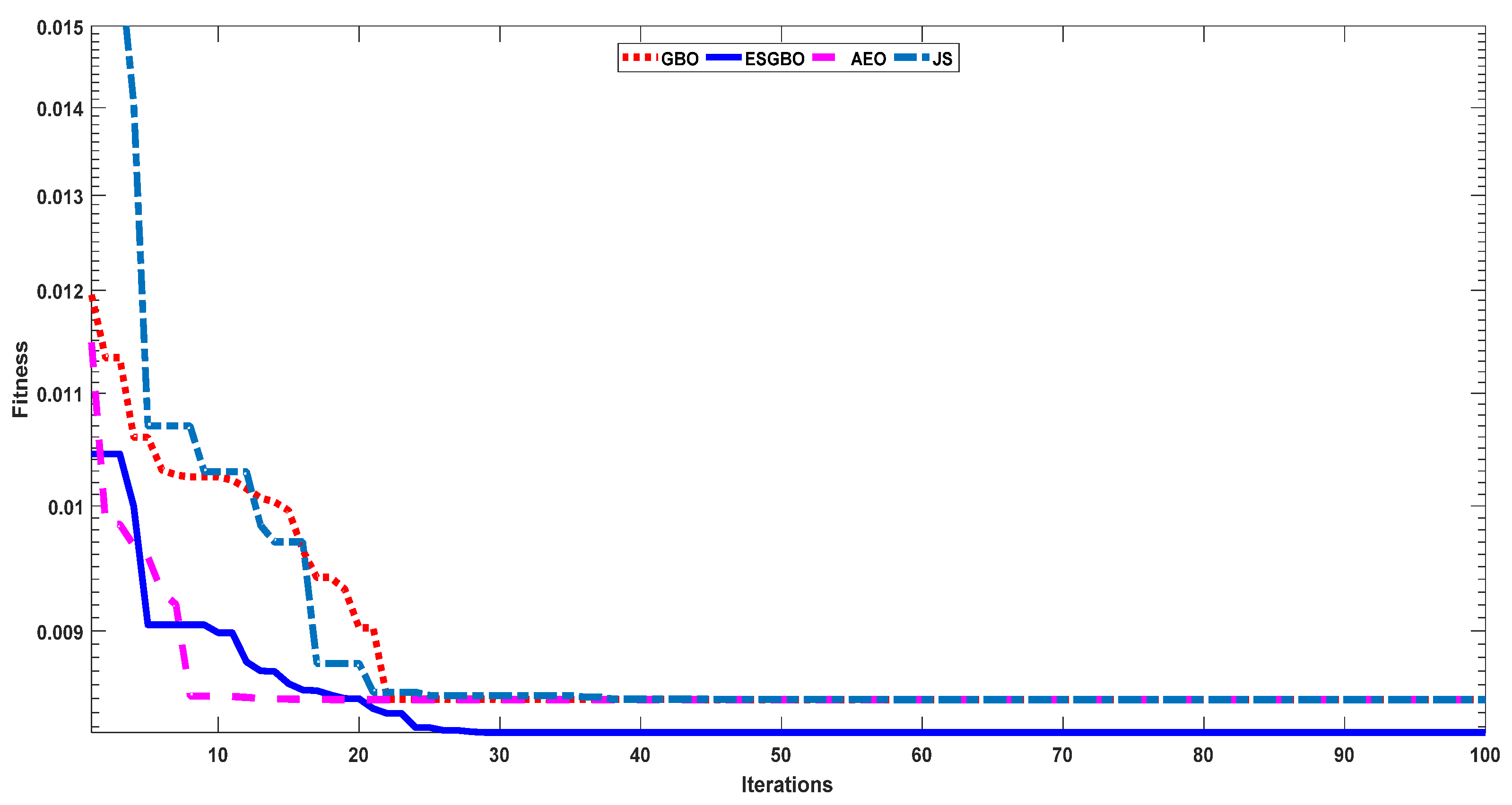
Figure 20.
Convergence curves of all algorithms for IOM.
Figure 20.
Convergence curves of all algorithms for IOM.
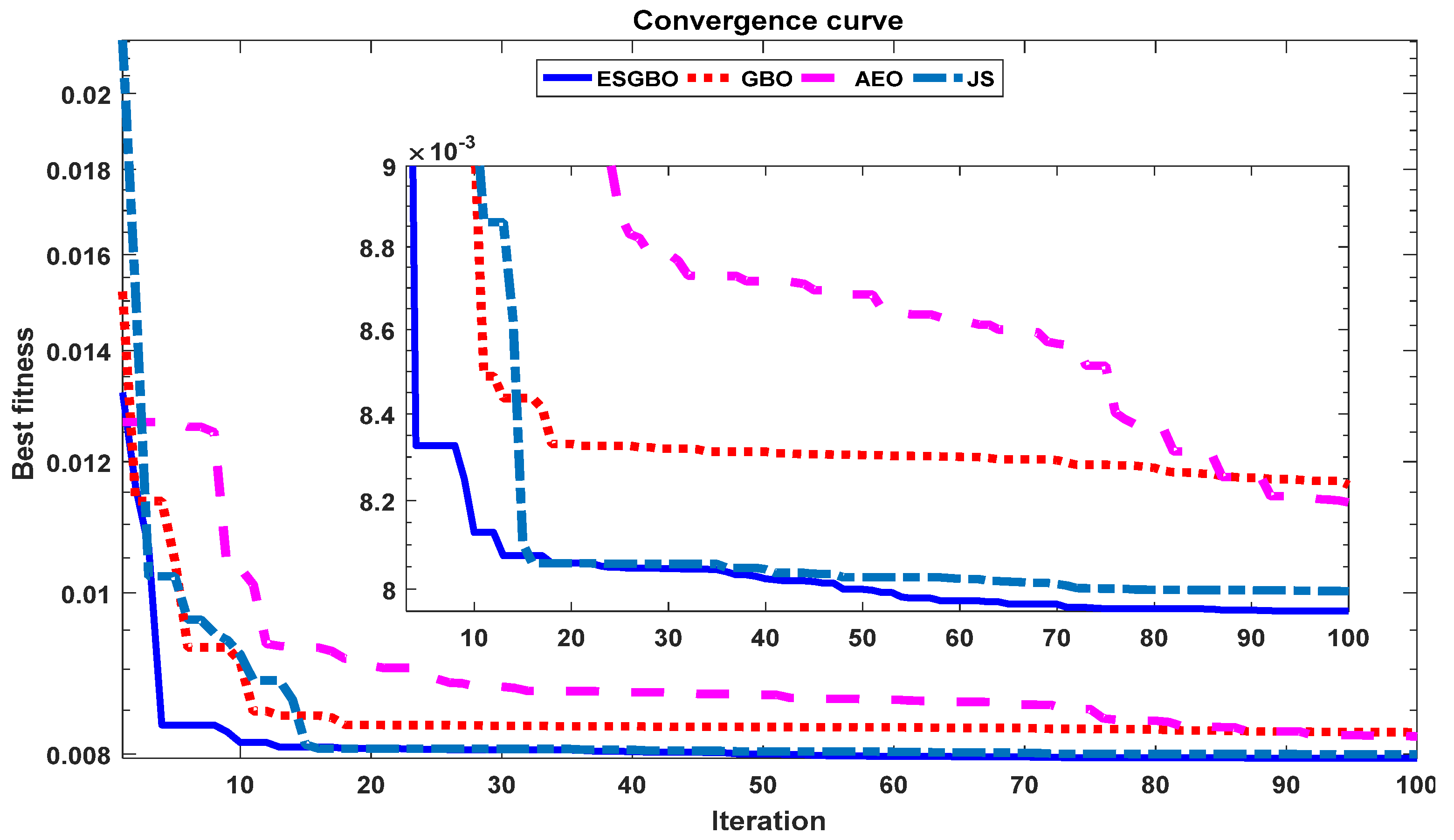
Figure 21.
Convergence curves of all algorithms for FOM.
Figure 21.
Convergence curves of all algorithms for FOM.
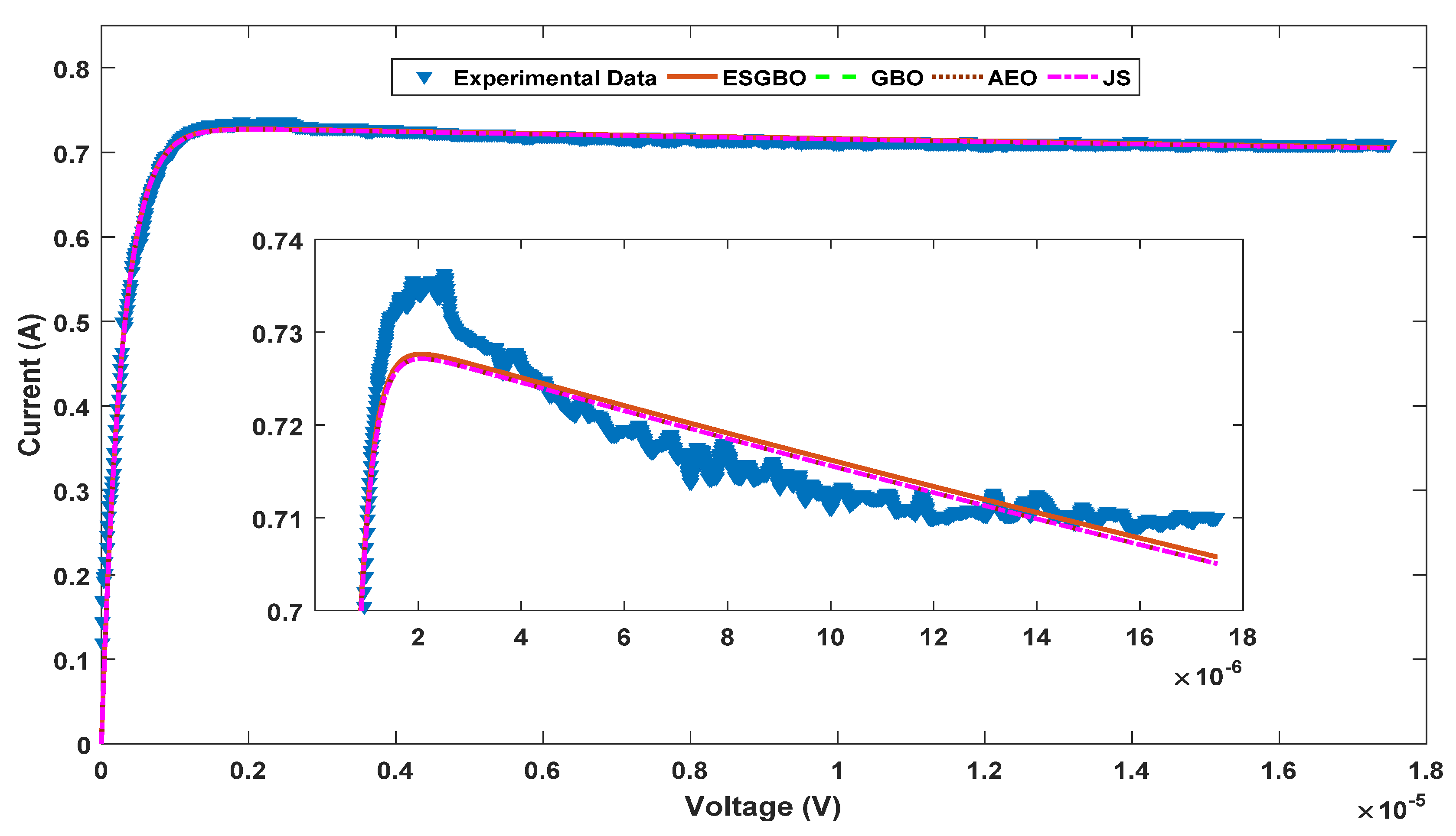
Figure 22.
Load current curve of real data and the estimated IOM by different algorithms.
Figure 22.
Load current curve of real data and the estimated IOM by different algorithms.
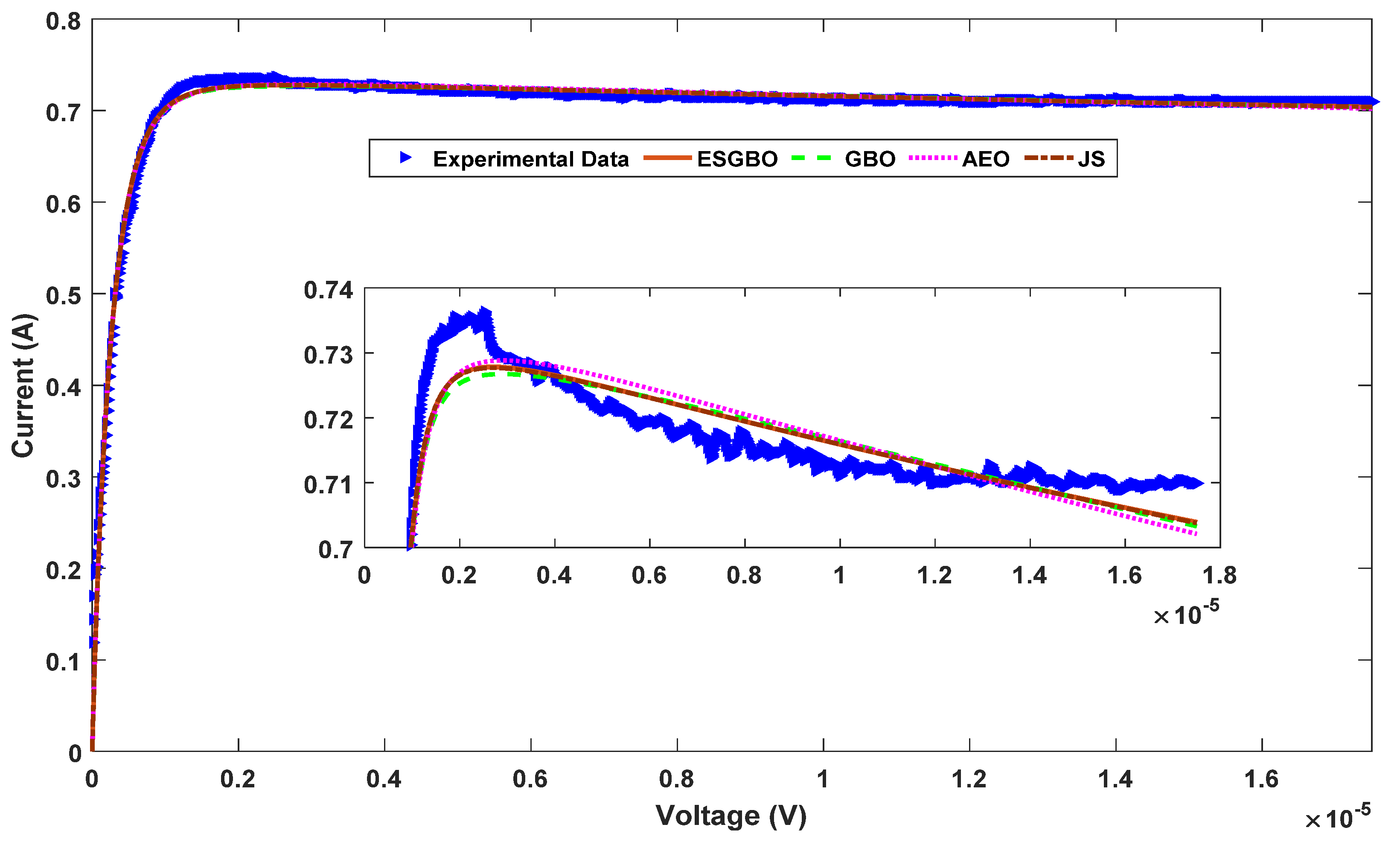
Figure 23.
Load current curve of real data and the estimated FOM by different algorithms.
Figure 23.
Load current curve of real data and the estimated FOM by different algorithms.
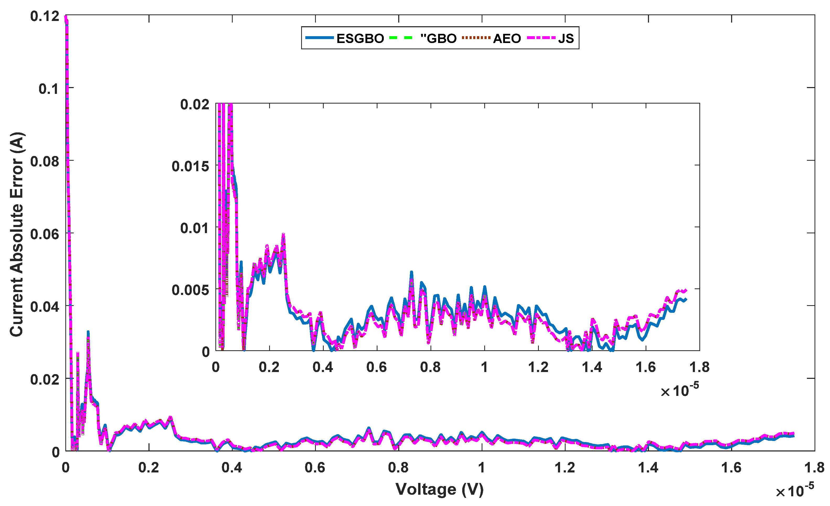
Figure 24.
Current absolute error of the estimated IOM by different algorithms.
Figure 24.
Current absolute error of the estimated IOM by different algorithms.
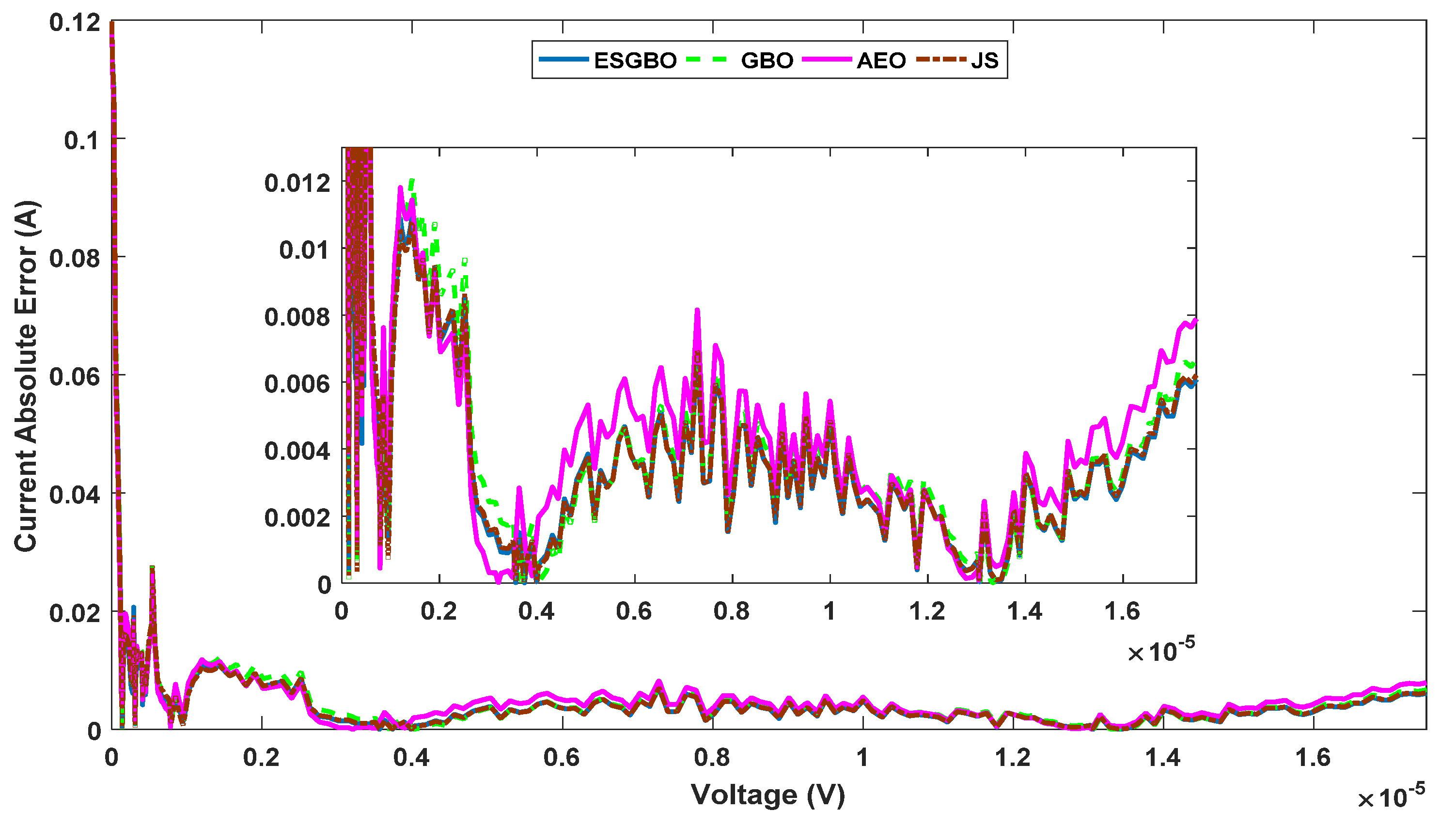
Figure 25.
Current absolute error of the estimated FOM by different algorithms.
Figure 25.
Current absolute error of the estimated FOM by different algorithms.
Table 1.
The statistical results of unimodal benchmark functions using the proposed technique and other well-known algorithms.
Table 1.
The statistical results of unimodal benchmark functions using the proposed technique and other well-known algorithms.
| Function | ESCGBO | GBO | WHO | EO |
|---|
| F1 | Best | 2.20 × 10−136 | 1.44 × 10−136 | 2.83 × 10−57 | 3.89 × 10−51 |
| Worst | 1.14 × 10−129 | 6.32 × 10−128 | 3.53 × 10−47 | 6.09 × 10−47 |
| Mean | 1.33 × 10−130 | 7.41 × 10−129 | 1.78 × 10−48 | 4.11 × 10−48 |
| std | 3.38 × 10−130 | 1.86 × 10−128 | 7.90 × 10−48 | 1.36 × 10−47 |
| F2 | Best | 2.31 × 10−71 | 2.89 × 10−70 | 8.31 × 10⁻³³ | 5.47 × 10⁻²⁹ |
| Worst | 2.33 × 10−65 | 1.84 × 10−66 | 9.82 × 10⁻²⁹ | 1.3 × 10⁻²⁷ |
| Mean | 1.39 × 10−66 | 2.39 × 10−67 | 1.39 × 10⁻²⁹ | 3.65 × 10⁻²⁸ |
| std | 5.2 × 10−66 | 4.92 × 10−67 | 2.48 × 10⁻²⁹ | 3.47 × 10⁻²⁸ |
| F3 | Best | 8.7 × 10−116 | 1.6 × 10−115 | 6.42 × 10−36 | 5.41 × 10⁻¹⁷ |
| Worst | 6.7 × 10−104 | 3.9 × 10−101 | 6.83 × 10⁻²⁸ | 1.39 × 10⁻¹¹ |
| Mean | 3.4 × 10−105 | 1.9 × 10−102 | 5.22 × 10⁻²⁹ | 2.34 × 10⁻¹² |
| std | 1.5 × 10−104 | 8.7 × 10−102 | 1.66 × 10⁻²⁸ | 4.08 × 10⁻¹² |
| F4 | Best | 1.58 × 10−64 | 8.91 × 10−64 | 5.07 × 10⁻²² | 4 × 10⁻¹⁴ |
| Worst | 3.03 × 10−58 | 1.63 × 10−59 | 3.71 × 10⁻¹⁹ | 6.87 × 10⁻¹² |
| Mean | 1.72 × 10−59 | 1.6 × 10−60 | 4.56 × 10⁻²⁰ | 1.2 × 10⁻¹² |
| std | 6.75 × 10−59 | 3.65 × 10−60 | 9.74 × 10⁻²⁰ | 1.77 × 10⁻¹² |
| F5 | Best | 19.99698 | 18.52388 | 23.60955 | 24.44135 |
| Worst | 25.02491 | 24.02389 | 86.19444 | 25.0421 |
| Mean | 21.68888 | 21.22658 | 34.30228 | 24.81639 |
| std | 1.324568 | 1.169705 | 20.97713 | 0.201379 |
| F6 | Best | 1.14 × 10⁻⁹ | 5.23 × 10⁻⁹ | 3.67 × 10⁻⁸ | 1.39 × 10⁻⁸ |
| Worst | 1.61 × 10⁻⁷ | 1.07 × 10⁻⁶ | 2.02 × 10⁻⁵ | 3.8 × 10⁻⁷ |
| Mean | 3.35 × 10⁻⁸ | 7.89 × 10⁻⁸ | 1.42 × 10⁻⁶ | 9.07 × 10⁻⁸ |
| std | 3.91 × 10⁻⁸ | 2.35 × 10⁻⁷ | 4.46 × 10⁻⁶ | 9.27 × 10⁻⁸ |
| F7 | Best | 0.000176 | 0.000111 | 4.5 × 10⁻⁵ | 9.73 × 10⁻⁵ |
| Worst | 0.001732 | 0.001663 | 0.00184 | 0.001432 |
| Mean | 0.000578 | 0.000528 | 0.000857 | 0.00068 |
| std | 0.000427 | 0.000392 | 0.000514 | 0.000358 |
Table 2.
The statistical results of multimodal benchmark functions using the proposed technique and other well-known algorithms.
Table 2.
The statistical results of multimodal benchmark functions using the proposed technique and other well-known algorithms.
| Function | ESCGBO | GBO | WHO | EO |
|---|
| F8 | Best | −1881.33 | −1909.05 | −1789.02 | −1798.26 |
| Worst | −1668.99 | −1659.76 | −1600.49 | −1715.16 |
| Mean | −1733.03 | −1771.42 | −1705.23 | −1751.04 |
| Std | 54.18392 | 83.01581 | 49.62292 | 21.99425 |
| F9 | Best | 0.00 | 0.00 | 0.00 | 0.00 |
| Worst | 0.00 | 0.00 | 0.00 | 0.00 |
| Mean | 0.00 | 0.00 | 0.00 | 0.00 |
| Std | 0.00 | 0.00 | 0.00 | 0.00 |
| F10 | Best | 8.88 × 10⁻¹⁶ | 8.88 × 10⁻¹⁶ | 8.88 × 10⁻¹⁶ | 20 |
| Worst | 8.88 × 10⁻¹⁶ | 8.88 × 10⁻¹⁶ | 20.00111 | 20 |
| Mean | 8.88 × 10⁻¹⁶ | 8.88 × 10⁻¹⁶ | 1.005259 | 20 |
| Std | 0.00 | 0.00 | 4.471221 | 1.23 × 10⁻¹⁰ |
| F11 | Best | 0.00 | 0.00 | 0.00 | 0.00 |
| Worst | 0.00 | 0.00 | 0.00 | 0.00 |
| Mean | 0.00 | 0.00 | 0.00 | 0.00 |
| Std | 0.00 | 0.00 | 0.00 | 0.00 |
| F12 | Best | 9.51 × 10⁻¹² | 1.45 × 10⁻¹⁰ | 1.18 × 10⁻¹¹ | 1.42 × 10⁻¹⁰ |
| Worst | 1.62 × 10⁻⁷ | 0.103669 | 0.103669 | 1.98 × 10⁻⁷ |
| Mean | 9.05 × 10⁻⁹ | 0.005183 | 0.01555 | 1.25 × 10⁻⁸ |
| Std | 3.61 × 10⁻⁸ | 0.023181 | 0.037979 | 4.37 × 10⁻⁸ |
| F13 | Best | 9.97 × 10⁻⁹ | 2.29 × 10⁻⁸ | 7.36 × 10⁻⁸ | 1.63 × 10⁻⁸ |
| Worst | 0.054779 | 0.054779 | 0.397801 | 0.108359 |
| Mean | 0.01043 | 0.016351 | 0.035814 | 0.018527 |
| Std | 0.014444 | 0.019872 | 0.093881 | 0.037211 |
Table 3.
The statistical Results of composite benchmark functions using the proposed technique and other well-known algorithms.
Table 3.
The statistical Results of composite benchmark functions using the proposed technique and other well-known algorithms.
| Function | ESCGBO | GBO | WHO | EO |
|---|
| F14 | Best | 0.998004 | 0.998004 | 0.998004 | 0.998004 |
| Worst | 0.998004 | 0.998004 | 3.96825 | 0.998004 |
| Mean | 0.998004 | 0.998004 | 1.543534 | 0.998004 |
| Std | 0.00 | 0.00 | 0.936299 | 1.76 × 10⁻¹⁶ |
| F15 | Best | 0.000307 | 0.000307 | 0.000307 | 0.000307 |
| Worst | 0.001594 | 0.001223 | 0.020363 | 0.020363 |
| Mean | 0.000528 | 0.000445 | 0.001676 | 0.002359 |
| Std | 0.00046 | 0.000335 | 0.004424 | 0.006161 |
| F16 | Best | −1.03163 | −1.03163 | −1.03163 | −1.03163 |
| Worst | −1.03163 | −1.03163 | −1.03163 | −1.03163 |
| Mean | −1.03163 | −1.03163 | −1.03163 | −1.03163 |
| Std | 2.28 × 10⁻¹⁶ | 2.28 × 10⁻¹⁶ | 1.35 × 10⁻¹⁶ | 2.1 × 10⁻¹⁶ |
| F17 | Best | 0.397887 | 0.397887 | 0.397887 | 0.397887 |
| Worst | 0.397887 | 0.397887 | 0.397887 | 0.397887 |
| Mean | 0.397887 | 0.397887 | 0.397887 | 0.397887 |
| Std | 0.00 | 0.00 | 0.00 | 0.00 |
| F18 | Best | 3.00 | 3.00 | 3.00 | 3.00 |
| Worst | 3.00 | 3.00 | 3.00 | 3.00 |
| Mean | 3.00 | 3.00 | 3.00 | 3.00 |
| Std | 8.7 × 10⁻¹⁶ | 4.2 × 10⁻¹⁶ | 5.85 × 10⁻¹⁶ | 6.76 × 10⁻¹⁶ |
| F19 | Best | −0.30048 | −0.30048 | −0.30048 | −0.30048 |
| Worst | −0.30048 | −0.30048 | −0.30048 | −0.30048 |
| Mean | −0.30048 | −0.30048 | −0.30048 | −0.30048 |
| Std | 1.14 × 10⁻¹⁶ | 1.14 × 10⁻¹⁶ | 1.14 × 10⁻¹⁶ | 1.14 × 10⁻¹⁶ |
| F20 | Best | −3.322 | −3.322 | −3.322 | −3.322 |
| Worst | −3.2031 | −3.2031 | −3.08668 | −1.84092 |
| Mean | −3.28633 | −3.28633 | −3.31023 | −3.12852 |
| Std | 0.055899 | 0.055899 | 0.052619 | 0.370083 |
| F21 | Best | −10.1532 | −10.1532 | −10.1532 | −10.1532 |
| Worst | −5.0552 | −5.0552 | −2.68286 | −5.0552 |
| Mean | −8.8787 | −8.3689 | −9.52706 | −8.88098 |
| Std | 2.264846 | 2.494761 | 1.966723 | 2.260817 |
| F22 | Best | −10.4029 | −10.4029 | −10.4029 | −10.4029 |
| Worst | −2.7659 | −5.08767 | −2.75193 | −2.7659 |
| Mean | −7.82681 | −8.5426 | −8.96998 | −9.75532 |
| Std | 2.973254 | 2.601082 | 2.948831 | 2.02859 |
| F23 | Best | −10.5364 | −10.5364 | −10.5364 | −10.5364 |
| Worst | −5.12848 | −2.80663 | −2.87114 | −2.42173 |
| Mean | −9.18443 | −8.25715 | −9.148 | −10.1307 |
| Std | 2.402536 | 2.907055 | 2.855393 | 1.814497 |
Table 4.
CPU time (s) of four algorithms on 23 benchmark functions.
Table 4.
CPU time (s) of four algorithms on 23 benchmark functions.
| | ESCGBO | GBO | WHO | EO |
|---|
| F1 | 2.24173 | 2.045234 | 1.666734 | 0.340013 |
| F2 | 1.831693 | 1.549915 | 1.43607 | 0.3331 |
| F3 | 2.615374 | 1.913063 | 1.671268 | 0.365052 |
| F4 | 1.945816 | 1.773811 | 2.09404 | 0.35823 |
| F5 | 2.032641 | 2.028365 | 1.704013 | 0.414698 |
| F6 | 1.88023 | 1.661728 | 1.679613 | 0.326943 |
| F7 | 2.077834 | 1.637886 | 1.454167 | 0.371617 |
| F8 | 1.795602 | 1.540629 | 1.430021 | 0.341869 |
| F9 | 1.842514 | 1.602524 | 1.657841 | 0.3381 |
| F10 | 1.761122 | 1.503307 | 1.394121 | 0.35016 |
| F11 | 1.780045 | 1.608481 | 1.64313 | 0.416369 |
| F12 | 1.746382 | 1.505388 | 1.366705 | 0.33033 |
| F13 | 1.99615 | 1.835235 | 1.43058 | 0.352283 |
| F14 | 2.417839 | 1.952414 | 1.608765 | 0.561999 |
| F15 | 1.985862 | 1.682823 | 2.037507 | 0.96656 |
| F16 | 1.754978 | 2.052051 | 1.407174 | 0.342419 |
| F17 | 1.72506 | 1.415434 | 1.564904 | 0.375495 |
| F18 | 2.746123 | 1.617294 | 2.4928 | 0.506535 |
| F19 | 1.891536 | 2.200207 | 1.470604 | 0.363025 |
| F20 | 1.792942 | 1.509464 | 1.532523 | 0.360518 |
| F21 | 2.009832 | 2.13849 | 1.56471 | 0.332705 |
| F22 | 2.330221 | 2.10297 | 2.356706 | 0.375617 |
| F23 | 2.127842 | 2.027598 | 1.530525 | 0.360371 |
Table 5.
Upper and lower constrains for all estimated parameters.
Table 5.
Upper and lower constrains for all estimated parameters.
| Parameter | Solar Cell |
|---|
| | Lower Limit | Upper Limit |
|---|
| Rs | 0 | 5 |
| Rsh | 0 | 100 |
| Iph | 0 | 2 |
| Is1 | 0 | 1 |
| Is2 | 0 | 1 |
| ɳ 1 | 1 | 2 |
| ɳ 2 | 1 | 2 |
Table 6.
Parameters setting for all compared algorithms.
Table 6.
Parameters setting for all compared algorithms.
| Algorithm | Control Prameters |
|---|
| ESCGBO | nP = 50 | pr = 0.5 | CM = 4 |
| GBO | nP = 50 | pr = 0.5 | CM = 4 |
| AEO | PopSize = 50 | r1 = rand | |
| JS | Npop = 50 | | |
| WHO | N = 50 | PS = 0.2 | PC = 0.13 |
| EO | Particles_no = 50 | a1 = 2, a2 = 1 | GP = 0.5 |
Table 7.
Estimated parameters and RMSE of ESCGBO and other algorithms for SDM model.
Table 7.
Estimated parameters and RMSE of ESCGBO and other algorithms for SDM model.
| | ESCGBO | GBO | AEO | JS |
|---|
| Rs (Ω) | 0.036377 | 0.036377 | 0.036377091 | 0.035989122 |
| Rsh (Ω) | 53.71853 | 53.71852 | 53.71853164 | 57.40304457 |
| Iph (A) | 0.760776 | 0.760776 | 0.76077553 | 0.760889273 |
| Is (A) | 3.23 × 10⁻⁷ | 3.23 × 10⁻⁷ | 3.23 × 10⁻⁷ | 3.61 × 10⁻⁷ |
| ɳ | 1.476894 | 1.476894 | 1.476894314 | 1.48800365 |
| RMSE | 0.000986022 | 0.000986022 | 0.000986022 | 0.001025784 |
Table 8.
Estimated parameters and RMSE of ESCGBO and other algorithms for DDM model.
Table 8.
Estimated parameters and RMSE of ESCGBO and other algorithms for DDM model.
| | ESCGBO | GBO | AEO | JS |
|---|
| Rs (Ω) | 0.036742647 | 0.036375073 | 0.036706957 | 0.035338785 |
| Rsh (Ω) | 55.50056767 | 53.68896189 | 55.32835695 | 54.95529664 |
| Iph (A) | 0.760781168 | 0.76077892 | 0.760783208 | 0.760597151 |
| Is1 (A) | 7.64 × 10⁻⁷ | 3.78 × 10⁻⁹ | 2.34 × 10⁻⁷ | 3.51 × 10⁻⁷ |
| Is2 (A) | 2.26 × 10⁻⁷ | 3.20 × 10⁻⁷ | 7.00 × 10⁻⁷ | 2.02 × 10⁻⁷ |
| ɳ 1 | 1.99999756 | 1.434376674 | 1.449582257 | 1.487619855 |
| ɳ 2 | 1.446849934 | 1.477724492 | 1.999999984 | 1.916132114 |
| RMSE | 0.000982418 | 0.000986029 | 0.000982451 | 0.00119615 |
Table 9.
The statistical results of SDM for all other algorithms.
Table 9.
The statistical results of SDM for all other algorithms.
| | Minimum | Average | Maximum | STD |
|---|
| ESCGBO | 0.000986022 | 0.000986026 | 0.000986032 | 5.507 × 10⁻⁹ |
| GBO | 0.000986022 | 0.000989455 | 0.000996022 | 5.688 × 10⁻⁶ |
| AEO | 0.000986022 | 0.000989555 | 0.000996022 | 5.608 × 10⁻⁶ |
| JS | 0.001025784 | 0.001525784 | 0.002025784 | 0.0005 |
Table 10.
The statistical results of DDM for all algorithms.
Table 10.
The statistical results of DDM for all algorithms.
| | Minimum | Average | Maximum | STD |
|---|
| ESCGBO | 0.000982418 | 0.000982454 | 0.000982518 | 5.507 × 10⁻⁸ |
| GBO | 0.000986029 | 0.000990032 | 0.000997039 | 6.088 × 10⁻⁶ |
| AEO | 0.000982451 | 0.000988451 | 0.000992451 | 5.291 × 10⁻⁶ |
| JS | 0.00110615 | 0.001469483 | 0.00210615 | 0.00055 |
Table 11.
Upper and lower constrains for all estimated parameters.
Table 11.
Upper and lower constrains for all estimated parameters.
| Parameter | Solar Cell |
|---|
| | Lower Limit | Upper Limit |
|---|
| Rc | 0 | 20 |
| C | 2 × 10⁻⁸ | 6 × 10⁻⁵ |
| L | 5 × 10⁻⁶ | 100 × 10−6 |
| α | 0.8 | 1.1 |
| β | 0.8 | 1.1 |
Table 12.
Estimated parameters of IOM model for all algorithms.
Table 12.
Estimated parameters of IOM model for all algorithms.
| | ESCGBO | GBO | AEO | JS |
|---|
| Rc | 5.583588 | 5.624748753 | 5.624748647 | 5.6247490 |
| C | 8.30 × 10⁻⁶ | 8.16 × 10⁻⁶ | 8.16 × 10⁻⁶ | 8.15726 × 10⁻⁶ |
| L | 7.43 × 10⁻⁶ | 7.47 × 10⁻⁶ | 7.47 × 10⁻⁶ | 7.47323 × 10⁻⁶ |
| RMSE | 0.008259444 | 0.008493067 | 0.008493067 | 0.008493067262 |
Table 13.
Estimated parameters of FOM model for all algorithms.
Table 13.
Estimated parameters of FOM model for all algorithms.
| | ESCGBO | GBO | AEO | JS |
|---|
| Rc | 4.617127916 | 5.005984283 | 4.550201539 | 4.698924713 |
| C | 5.81 × 10⁻⁵ | 5.04 × 10⁻⁶ | 1.46 × 10⁻⁵ | 4.08 × 10⁻⁵ |
| L | 1.50 × 10⁻⁵ | 1.35 × 10⁻⁵ | 1.73 × 10⁻⁵ | 1.44 × 10⁻⁵ |
| A | 0.8 | 1.026120535 | 0.917230623 | 0.833404373 |
| β | 0.950840763 | 0.957165925 | 0.940654537 | 0.953192785 |
| RMSE | 0.007951289 | 0.008236017 | 0.00819598 | 0.007995872 |


 ,
, 


