
Targeting Energy Efficiency through Air Conditioning Operational Modes for Residential Buildings in Tropical Climates, Assisted by Solar Energy and Thermal Energy Storage. Case Study Brazil


Abstract
:1. Introduction
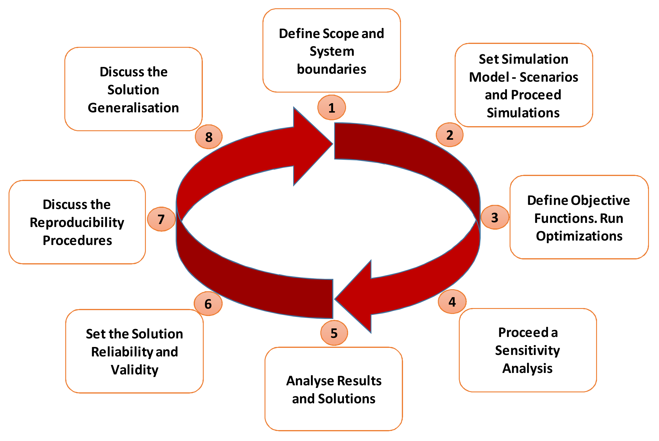
2. Materials and Methods
2.1. Scope and System Boundaries
2.2. Simulation Model, Scenarios, and Proceed Simulations
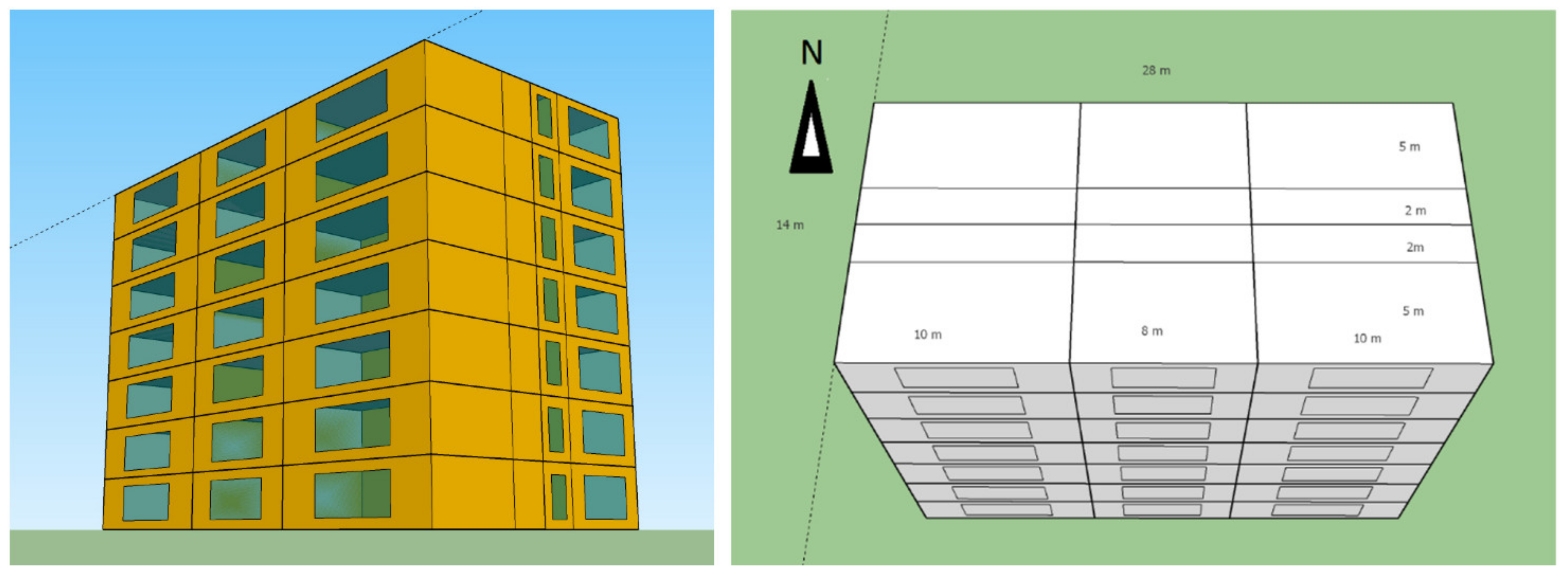
- Hypothetical building model, initially designed in the SketchUp and configured via TRNSYS Building tool, for the calculation of the building cooling demand;
- Cooling system model, responsible to supply the building cooling demand and calculate the whole building electrical energy demand. This model simulates ASHRAE operational modes for the chiller/TES set and allows to choose each of the four selected scenarios;
- PV/grid model, responsible to supply the building electrical energy demand for the different scenarios and calculate the LCC and payback. Interacts with the GenOpt for the optimization process.
- Base Case: grid + chiller full capacity (no TES);
- Scenario 1: PV + grid + chiller partial time + TES full storage load;
- Scenario 2: PV + grid + chiller partial capacity + TES partial load (load leveled);
- Scenario 3: PV + grid + chiller partial capacity + TES partial load (demand limiting).
2.3. Objective Functions and Optimization
- Ct = Sum of all relevant costs occurring in year t (EUR);
- N = Length of study period (years);
- i = Nominal discount rate (%).
- r = Real discount rate (%);
- i = Nominal discount rate (%);
- I = General energy price inflation (%).
2.4. Sensitivity Analysis
3. Case Study
3.1. Building Description
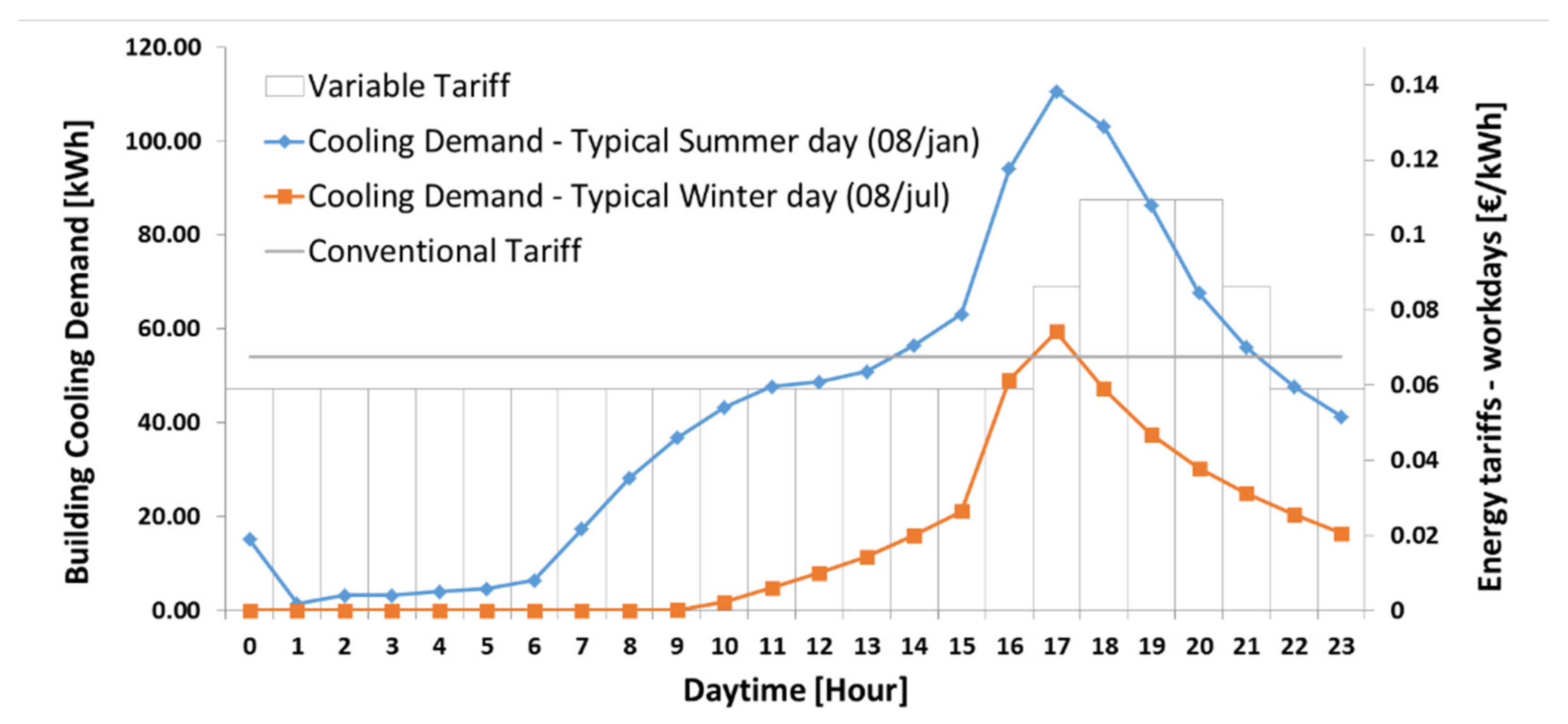
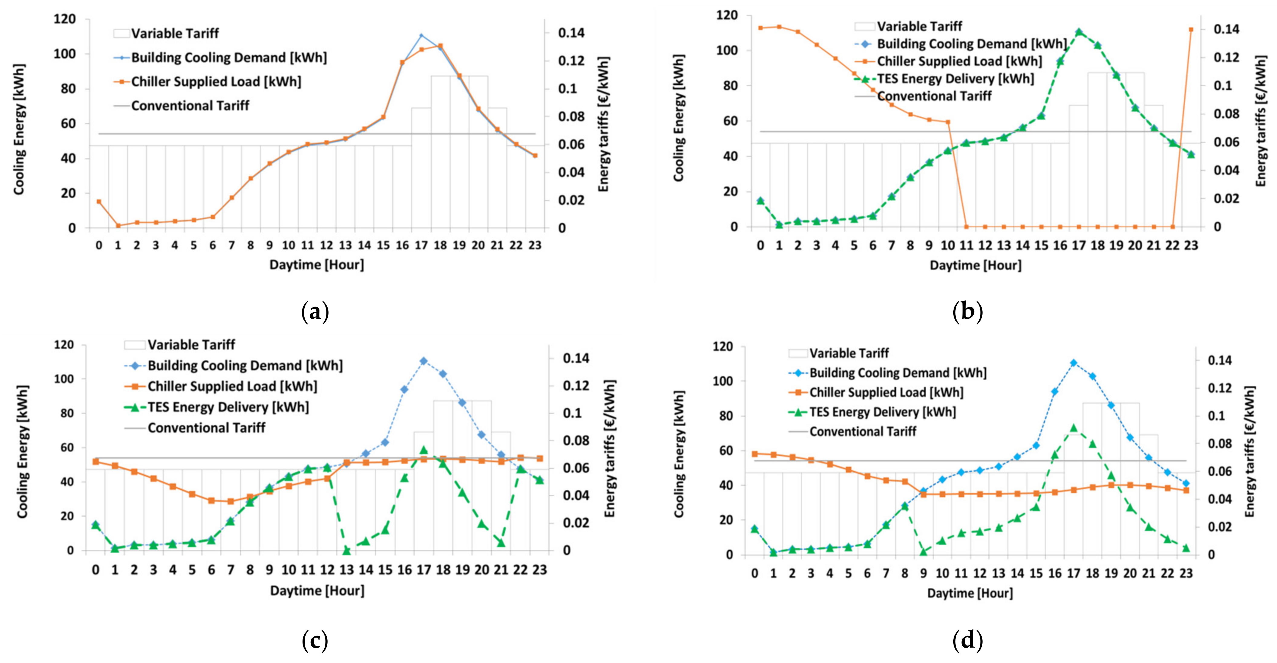
3.2. Grid Electricity Tariffs
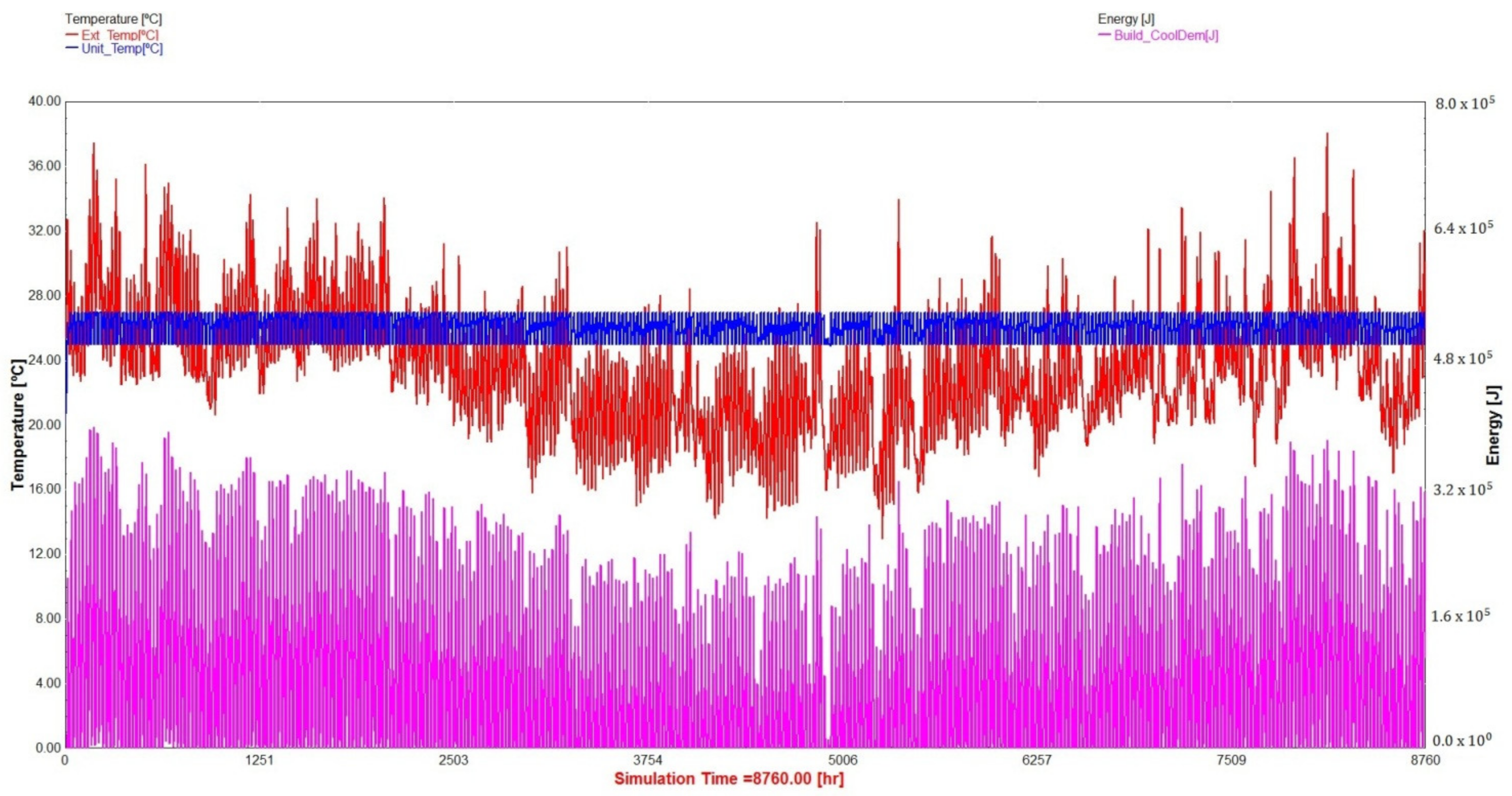
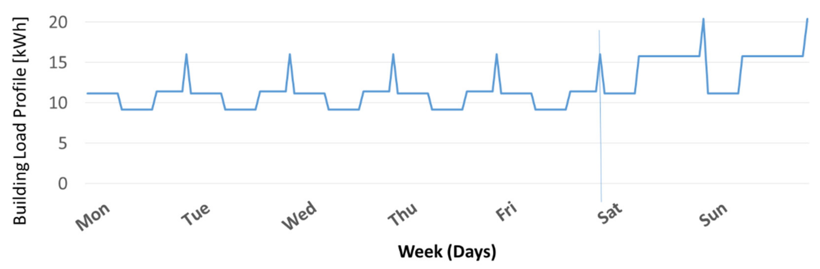
3.3. Building Cooling Demand Profile
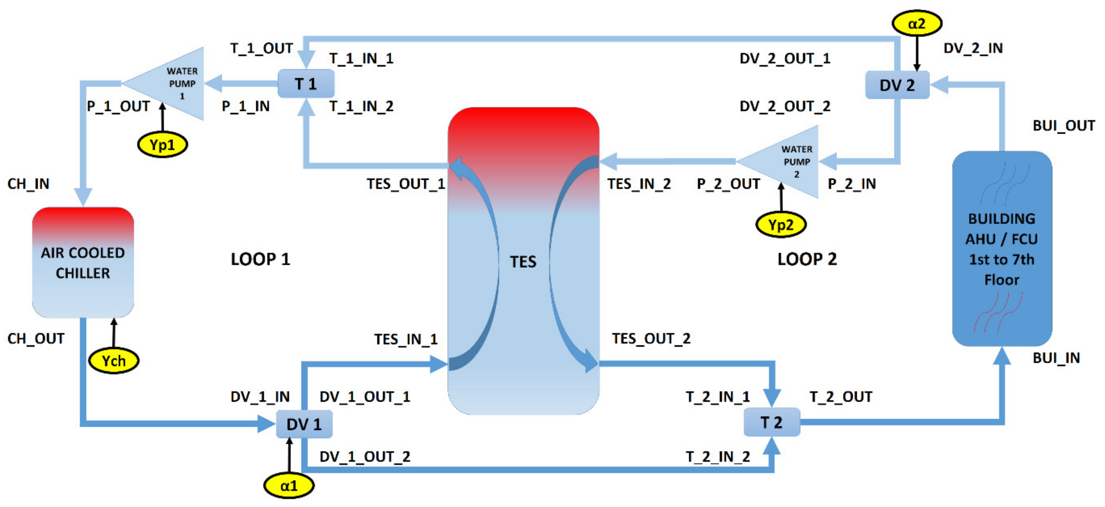
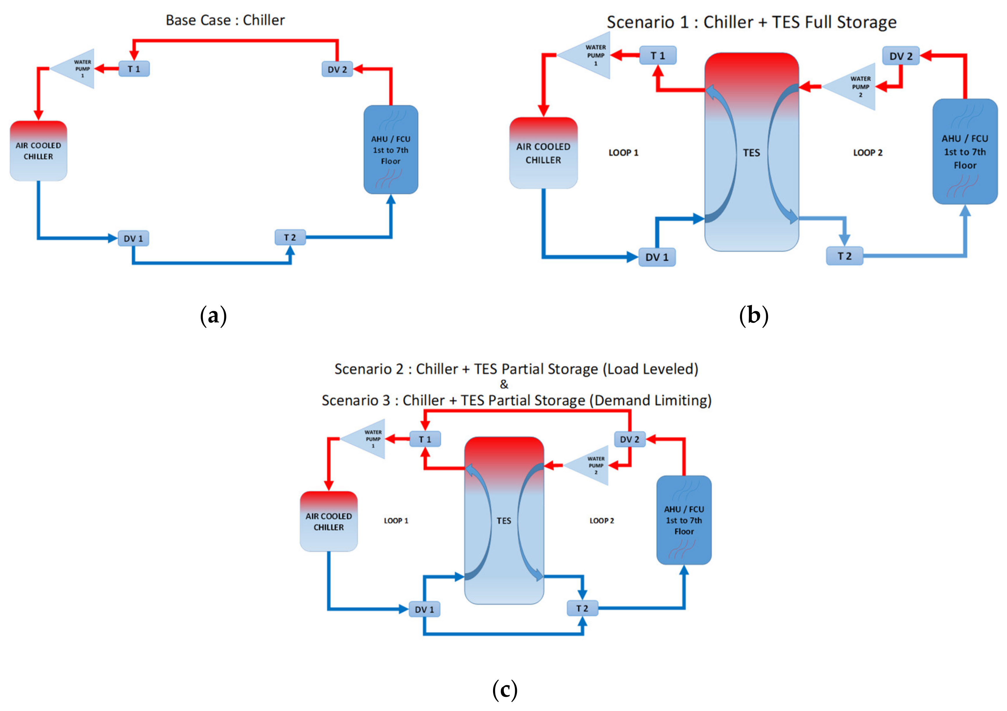
3.4. Cooling System Overview
- Air-cooled chiller (condenser, evaporator, and cooling fans);
- Variable speed pump (chilled water);
- Thermal energy storage—TES_IN_1 and TES_OUT_1.
- Thermal energy storage—TES_IN_2 and TES_OUT_2;
- Variable speed pump (chilled water);
- Building air handling unit (AHU) and fan coil unit (FCU).
- Loop 1: the chiller and pump work based on signals (schedule and the TES top temperature);
- Loop 2: the pump works based on the signal (the required water amount for building load demand).
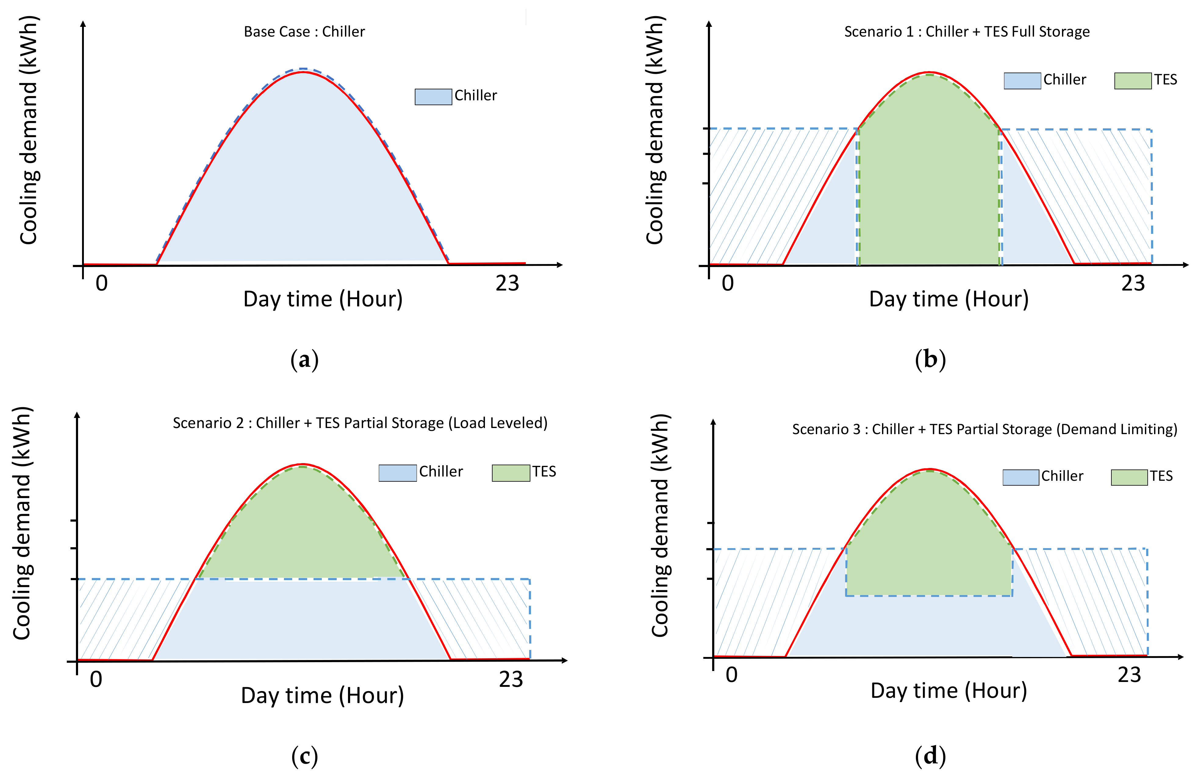
3.4.1. Base Case—Chiller Only (No Storage)
- = Signal control value of Water Pump 1 at LOOP 1 [0 ≤ ≤ 1];
- = Building cooling demand (kWh);
- Water mass necessary to supply the building cooling demand (kg);
- = Pump flow rate capacity kg/h or m3/h;
- = Specific heat for water;
- = Cool coil temperature difference ( (°C).
- = Building maximum cooling demand (kWh);
- = Specific heat for water (kWh/kg°C);
- = Cool coil temperature difference ( (°C);
- = Pump flow rate capacity kg/h or m3/h;
- = Water density (kg/m3).
3.4.2. Scenario 1—Chiller Full Capacity + TES Full Storage Load
- = TES volume (m3);
- = Building maximum cooling demand (kWh/day);
- = Specific heat for water (kWh/kg °C);
- = TES temperature difference ( (°C);
- = Water density (kg/m3);
- .
3.4.3. Scenario 2—Chiller Partial Capacity + TES Partial Storage (Load Leveled)
3.4.4. Scenario 3—Chiller Partial Capacity + TES Partial Storage (Demand Limiting)
- Chiller capacity and chiller operation schedule;
- TES volume and height;
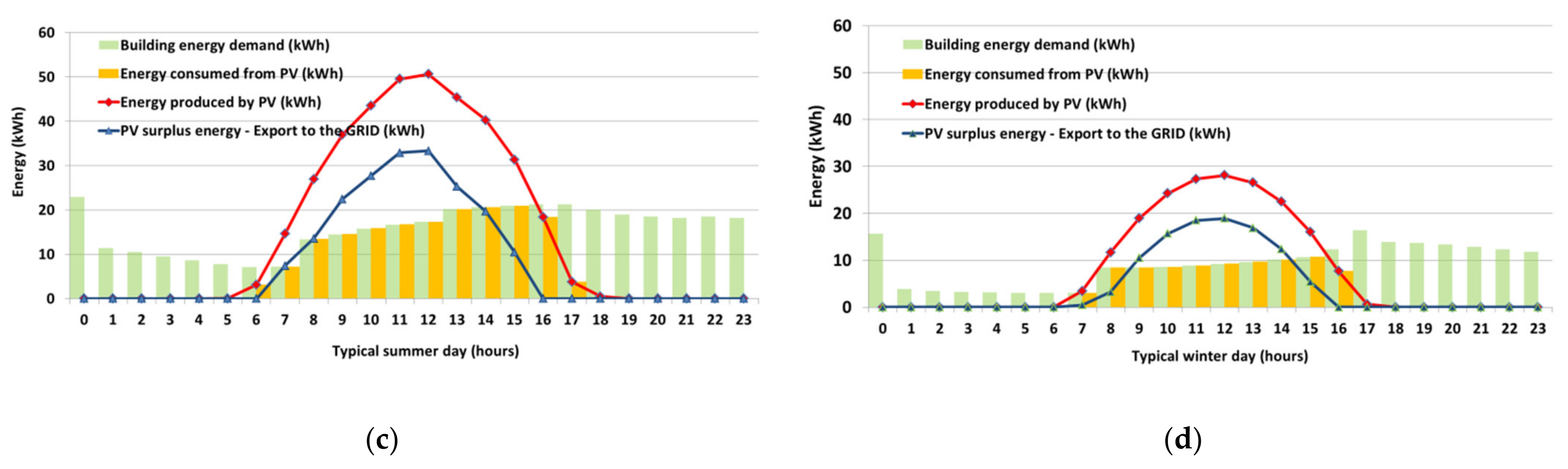
3.5. PV System Overview
4. Results and Discussion
4.1. Analyze Results and Solutions
4.1.1. Base Case—PV + Grid + Chiller (No Storage)
4.1.2. Scenario 1—PV + Grid + Chiller + TES Full Storage Load
4.1.3. Scenario 2—PV + Grid + Chiller Partial Capacity + TES Partial Load (Load Leveled)
4.1.4. Scenario 3—PV + Grid + Chiller Partial Capacity + TES Partial Load (Demand Limiting)
4.1.5. Annual Energy and Power Analysis (No PV energy)
4.1.6. PV Energy Analysis
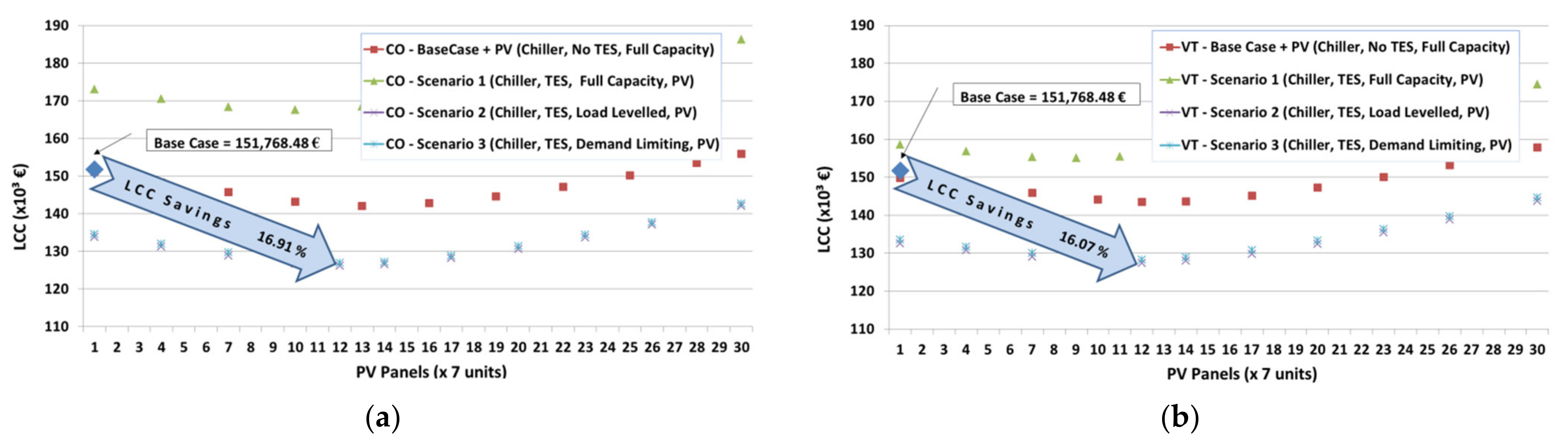
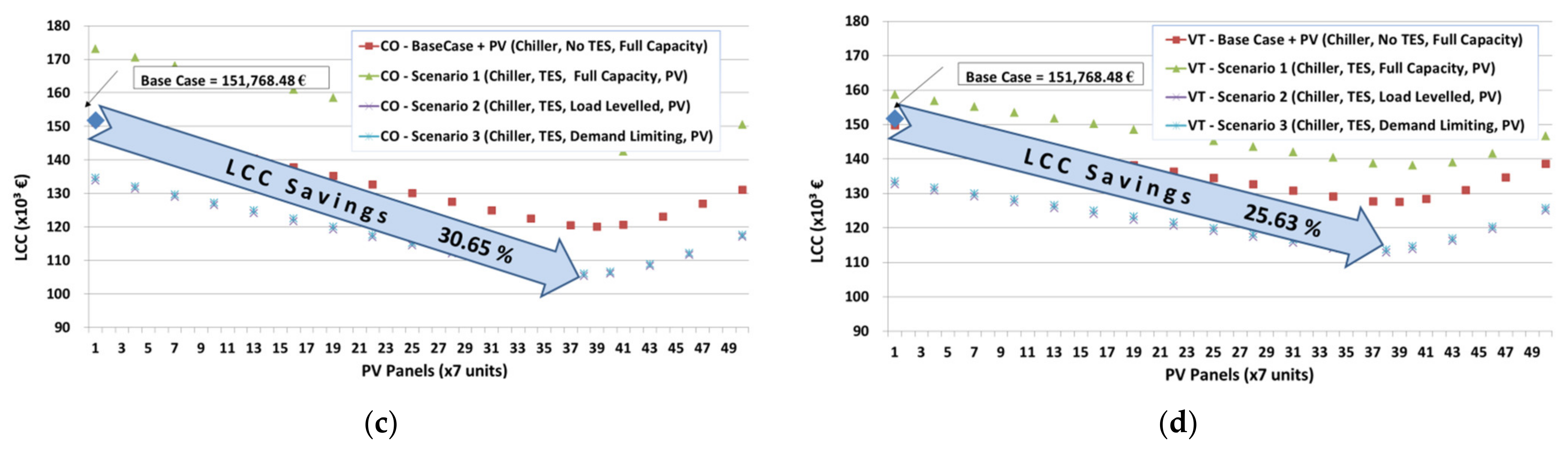
4.1.7. Life Cycle Costing Analysis
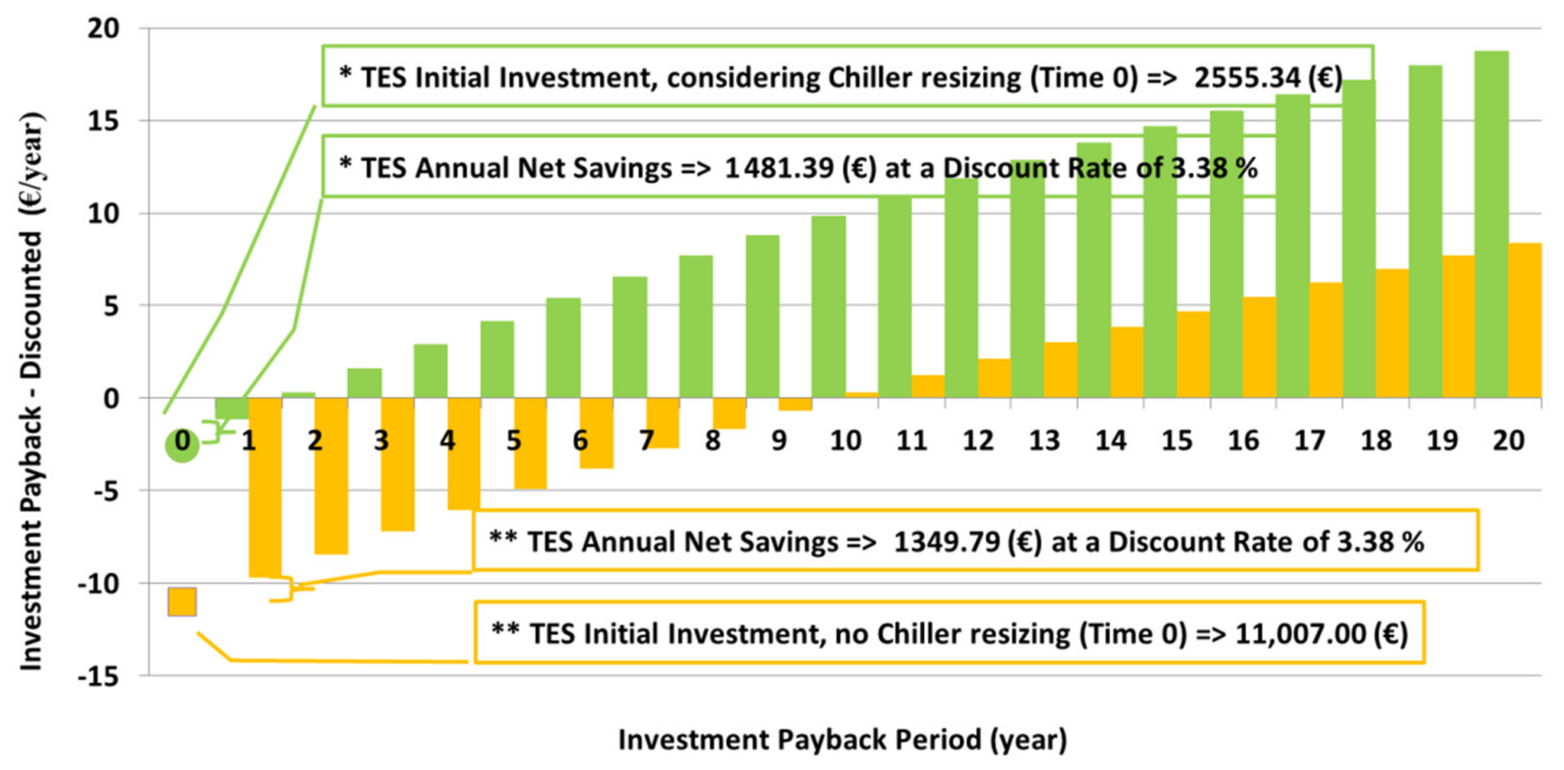
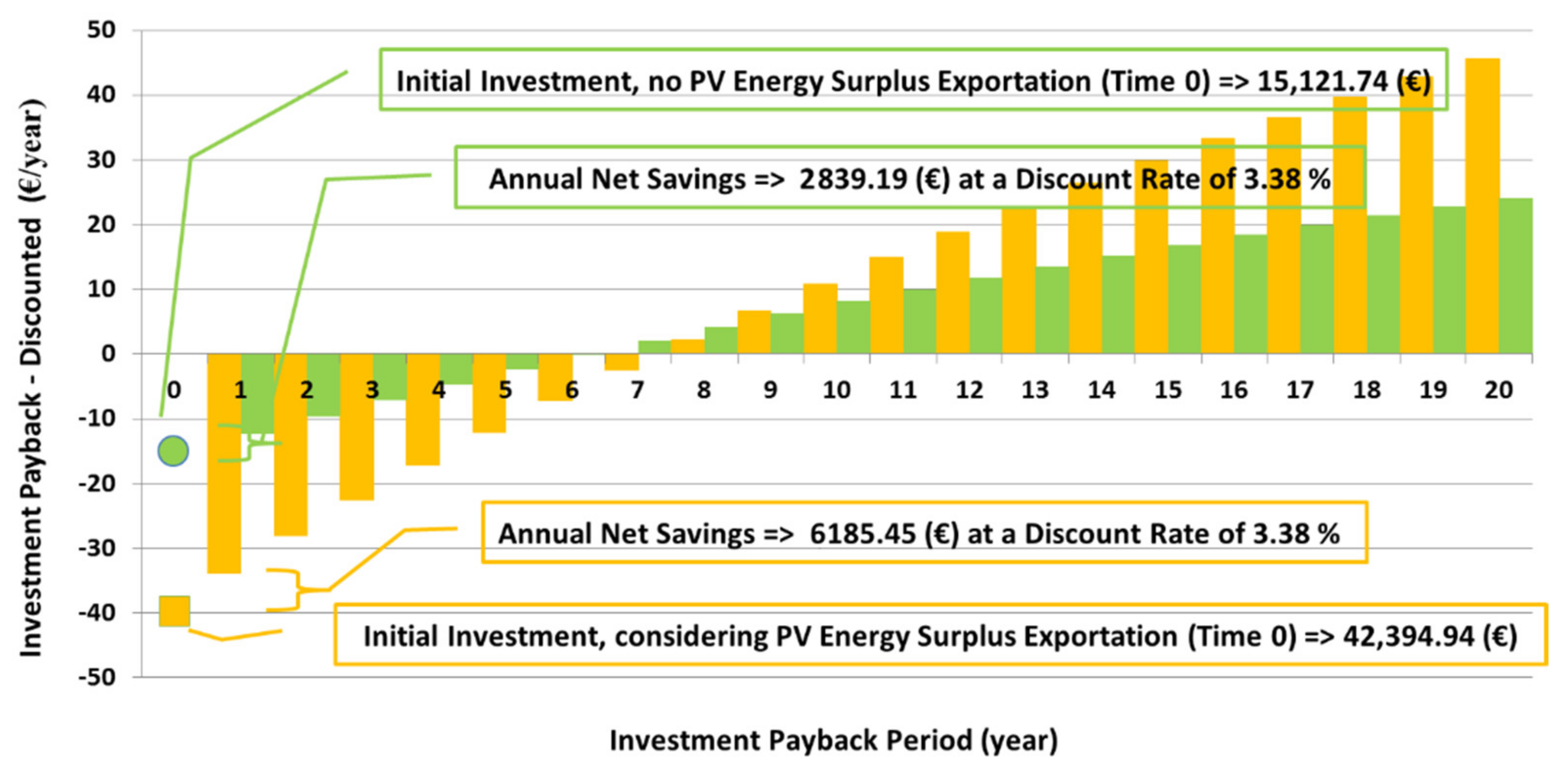
4.1.8. Payback Period Analysis
5. Conclusions
Author Contributions
Funding
Institutional Review Board Statement
Informed Consent Statement
Data Availability Statement
Acknowledgments
Conflicts of Interest
Nomenclature
| AHU | Air Handling Unit |
| AM | Advanced Metering |
| ASHRAE | American Society of Heating, Cooling, and Air Conditioning Engineers |
| CO | Conventional Electricity Tariff |
| DOE | Department of Energy |
| DR | Demand Response |
| EEAF | Energy Efficiency Analysis Framework |
| FCU | Fan Coil Unit |
| HVAC | Heating, Ventilating, and Air Conditioning |
| GENOPT | Generic Optimization Program |
| GRID | Electrical grid |
| LCC | Life Cycle Costing |
| MOO | Multi-objective Optimization |
| NM | Net Metering |
| NREL | National Renewable Energy Laboratory |
| NZEB | Net Zero Energy Building |
| PB | Payback Period |
| PV | Photovoltaic |
| TRNSYS | Transient System Simulation Program |
| SHGC | Solar Heat Gain Coefficient |
| SOO | Single Objective Optimization |
| TES | Thermal Energy Storage |
| VT | Variable Electricity Tariff |
| WWR | Window-to-Wall Ratio |
Appendix A. Energy Efficiency Analysis Framework (EEAF)
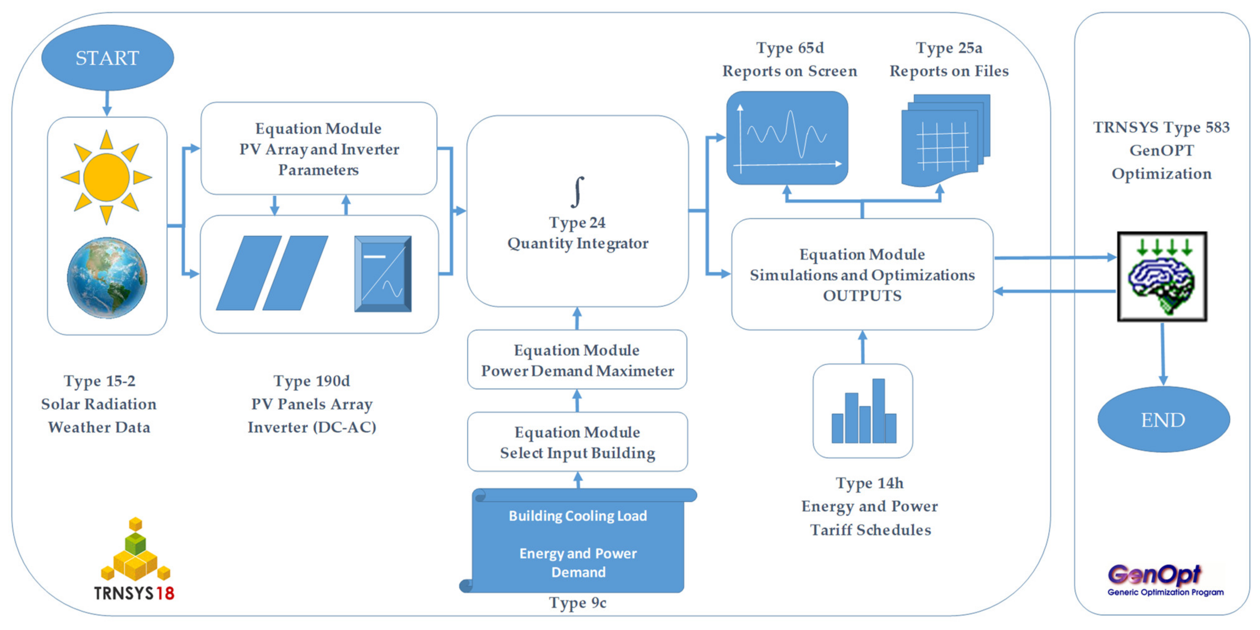
Appendix B. Main TRNSYS Components

| Model: Name | Description | Function |
|---|---|---|
| Type 15-2: Weather Data Processor | Combines data reading, radiation processing, and sky temperature calculations. | Simulates the solar energy potential as input for the PV array using Energy Plus Weather Data [41] from different locations (Brazil) on an hourly basis for one year. |
| Type 56b: Building | Aggregates the information from the building model drawn in the Trimble SketchUp 2016 software and exported via 3DTrnsys plugin to TRNSYS Simulation Studio. | Simulates the residential building energy and power demand on an hourly basis for one year. Supply energy and power inputs to Type 9c. |
| Type 9c: Data Reader for Generic Data Files | Serves the purpose of reading data at regular time intervals from a data file, converting it to a desired system of units, and making it available to other TRNSYS components. | Reads the electrical hourly energy and power data files. |
| Type 190d: PV Array MPPT and Inverter (DC to AC) | Determines the electrical performance of a photovoltaic array, based on the calculation method presented by DeSoto et al. [31]. | Simulates different array configurations categorized into scenarios to support the building energy demand. |
| Type 14h: Time-Dependent Forcing Function | Employs a time-dependent forcing function, which has a repeated pattern. Discrete data points indicating the value of the function at various times throughout one cycle (e.g., one day) set the pattern of the forcing function. | Sets the Variable Tariff Schedule for the energy and power contracted to calculate the costs and proceed with the life cycle cost and payback optimizations for the different scenarios. |
| Type 24: Quantity Integrator | Integrates a series of quantities over a period. Each quantity integrator can have up to 500 inputs. It can reset either periodically throughout the simulation or after a specified number of hours or after each month of the year. | Summarizes the amount of energy consumption, power demand, and life cycle costing. |
| Type Equation: Algebraic, Logic, and Boolean Equations | Allows implementing calculations and formulas using equations. | Calculates the output integrated values from Type 24 (Integrator) and implement logical conditions for the different scenarios related, for example, to the use of solar energy or grid energy to support the energy consumption and power demand. It also calculates the life cycle costing and payback period of possible investments for each scenario. |
| Type 65d: Reports on screen | Allows visualization of the graphical results of the simulations at different time frames (e.g., hourly based graphics for 8760 h of simulation, or 1 year). | Displays simulations in real-time. |
| Type 25a: Printer—TRNSYS | Supplies units printed to an output file. | Exports the simulation and calculation results |
| Type 583: GenOpt Optimazation | Optimization program for the minimization of a cost functionthat is evaluated by the TRNSYS Simulation Studio. | The cost function is the function being optimized. The cost function measures a quantity that should be minimized, such as a building’s annual operation cost, a system’s energy consumption, or a norm between simulated and measured values in a data fitting process. The cost function is also called the objective function. |
Appendix C. Building Thermal Properties
| Material | Conductivity (kJ/hmK) | Capacity (kJ/kgK) | Density (°C) | Resistance (hm2K/kJ) |
|---|---|---|---|---|
| PLASTER_BOARD | 0.576 | 0.84 | 950 | - |
| FBRGLS_ASHRAE | 0.144 | 0.84 | 12 | - |
| WD_SIDN_ASHRAE | 0.504 | 0.90 | 530 | - |
| TIMBER_FLOOR_ASHRAE | 0.504 | 1.20 | 650 | - |
| RFDCK_ASHRAE | 0.504 | 0.90 | 530 | - |
| CONCRETE_SLAB | 4.068 | 1.00 | 1400 | - |
| INS_FLR_ASHRAE (Massless Layer) | - | - | - | 6.965 |
| Window Type | WWR (%) | SGHC (%) | U-Value (W/m2K) |
|---|---|---|---|
| Exterior Window 1 | 30 | 78.9 | 2.89 |
| Exterior Window 2 | 30 | 78.9 | 2.89 |
| Adjacent Window 1 | 30 | 78.9 | 2.89 |
| Adjacent Window 2 | 30 | 78.9 | 2.89 |
| Wall Type | Material | Total Thickness (m) | U-Value (W/m2K) |
|---|---|---|---|
| Boundary Wall | 0.090 | 0.508 | |
| PLASTER_BOARD | 0.012 | ||
| FBRGLS_ASHRAE | 0.066 | ||
| PLASTERBOARD | 0.012 | ||
| Adjacent Wall | 0.090 | 0.508 | |
| PLASTER_BOARD | 0.012 | ||
| FBRGLS_ASHRAE | 0.066 | ||
| PLASTERBOARD | 0.012 | ||
| Exterior Wall | 0.087 | 0.510 | |
| PLASTER_BOARD | 0.012 | ||
| FBRGLS_ASHRAE | 0.066 | ||
| WD_SIDN_ASHRAE | 0.009 | ||
| Exterior Roof | 0.141 | 0.316 | |
| PLASTER_BOARD | 0.010 | ||
| FBRGLS_ASHRAE | 0.112 | ||
| RFDCK_ASHRAE | 0.019 | ||
| Exterior Floor | 0.030 | 0.039 | |
| TIMBER_FLOOR_ASHRAE | 0.030 | ||
| INS_FLR_ASHRAE | |||
| Boundary Ceiling | 0.080 | 4.153 | |
| CONCRETE_SLAB | 0.080 | ||
| Adjacent Ceiling | 0.080 | 4.153 | |
| CONCRETE_SLAB | |||
| Boundary Floor | 0.030 | 0.039 | |
| TIMBER_FLOOR_ASHRAE | 0.030 | ||
| INS_FLR_ASHRAE | |||
| Ground Floor | 0.080 | 0.039 | |
| CONCRETE_SLAB | 0.080 | ||
| INS_FLR_ASHRAE |
Appendix D. Chillers Data
| % Load | Cooling Capacity (ton) | Compressor Input Power (kW) | Ambient Temperature (°C) | Energy Efficiency Rate EER |
|---|---|---|---|---|
| Chiller YACL0043 31.2 Ton (110 kW)—Base Case and Scenario 1 | ||||
| 100 | 31.2 | 31.7 | 35.0 | 10.7 |
| 75 | 25.1 | 19.5 | 28.5 | 13.2 |
| 50 | 17.6 | 10.7 | 20.4 | 17.1 |
| 25 | 9.7 | 4.6 | 12.8 | 21.5 |
| Chiller YACL0022 15.6 Ton (56 kW)—Scenarios 2 and 3 | ||||
| 100 | 15.6 | 17.6 | 35.0 | 10.3 |
| 50 | 9.7 | 5.6 | 20.4 | 18.8 |
| 1 ton = 12,000 Btu/h = 3.517 kW = 12,660.67 kJ/h | ||||
Appendix E. Chiller Calculation Comparison
Appendix F. Summary of Symbols and Indexes Used in the Equations and Diagrams
| BUI_IN: Building Cooled Water Input (m3/h) |
| BUI_OUT: Building Cooled Water Output (m3/h) |
| : Chiller Capacity (n = 0, 1, 2, 3; n = 0 for Base Case; n = 1, 2, 3 for Scenarios 1, 2, 3) (kW) or (ton) |
| Chiller Schedule Signal (0 ≤ signal ≤ 1) |
| CH_IN: Chiller Input (Water to be Cooled) (m3/h) |
| CH_OUT: Chiller Output (Cooled Water) (m3/h) |
| CO: Conventional Tariff—Power: (EUR/kW); Energy: (EUR/kWh) |
| Specific Heat for water [kWh/kg°C] |
| : Sum of all relevant costs occurring in year t (EUR) |
| ΔT) (°C) |
| DV_n: Flow Diverter (n = 1, 2) |
| DV_n_IN_p: Flow Diverter Input (n = 1, 2; p = 1, 2) (m3/h) |
| DV_n_OUT_p: Flow Diverter Output (n = 1, 2; p = 1, 2) (m3/h) |
| = Pump Fçow Rate Capacity (kg/h) or (m3/h); |
| i = Nominal Discount Rate (%) |
| I = General Energy Price Inflation (%). |
| LOOP_1: Chiller Side Water Loop |
| LOOP_2: Building Side Water Loop |
| m: Water mass (kg) |
| N: Length of study period (years); |
| Optm. Ct. Pw.: Optimal Value for the Contracted Power from the grid (kW) |
| P_n_IN: Water Pump Input (n = 1, 2) (m3/h) |
| P_n_OUT: Water Pump Output (n = 1, 2) (m3/h) |
| Building Cooling Demand [kWh] |
| : Building maximum cooling demand (kWh/day); |
| ρ: Water density (kg/m3) |
| r = Real Discount Rate (%) |
| Input Cool Coil Water Temperature (°C) |
| T_n: Tee Piece (n = 1, 2) |
| Output Cool Coil Water Temperature (°C) |
| TES_IN_n: TES Water Input (n = 1, 2) (m3/h) |
| TES_OUT_n: TES Water Output (n = 1, 2) (m3/h) |
| Total Pw.: Building Total Power Demanded (kW) |
| VT: Variable Tariff—Power: [ €/kW]; Energy: (EUR/kWh) |
| : TES volume (m3) |
| Ych: Chiller Control Signal (0 ≤ signal ≤ 1) |
| Yp_n: Water Pump Control Signal (n = 1, 2; 0 ≤ signal ≤ 1) |
| α_n: Flow Diverter Control Signal (n = 1, 2; 0 ≤ signal ≤ 1) |
Appendix G. TRNSYS Simulations and Optimizations Results. Base Case and Scenarios
| No PV | PV (No Energy Exportation) | PV (Energy Esportation—Net Metering) | |||||||||||||||||
|---|---|---|---|---|---|---|---|---|---|---|---|---|---|---|---|---|---|---|---|
| CO 1 | VT 2 | CO | VT | CO | VT | ||||||||||||||
| Chiller Cap ton | Chiller Cap kW | Chiller Inv EUR × 103 | TES Vol m3 | TES Inv EUR × 103 | LCC 20y EUR × 103 | LCC 20y EUR × 103 | PV (×7) NoExp | PV Inv EUR × 103 | LCC 20y EUR × 103 | PV (×7) NoExp | PV Inv EUR × 103 | LCC 20y EUR × 103 | PV (×7) EnExp | PV Inv EUR × 103 | LCC 20y EUR × 103 | PV (×7) EnExp | PV Inv EUR × 103 | LCC 20y EUR × 103 | |
| BCase | 30.17 | 106.10 | 16.9 | 0 | 0 | 151.8 3 | 150.3 | 13 | 13.6 | 142.1 | 12 | 12.6 | 143.6 | 39 | 40.8 | 120.0 | 39 | 40.8 | 127.6 |
| Scen 1 | 32.52 | 114.37 | 18.2 | 137.46 | 13.6 | 173.7 | 159.1 | 10 | 10.5 | 167.6 | 9 | 9.4 | 155.1 | 41 | 42.9 | 142.5 | 40 | 41.9 | 138.1 |
| Scen 2 | 15.08 | 53.06 | 8.4 | 110.07 | 11.0 | 134.4 | 133.0 | 12 | 12.6 | 126.1 | 12 | 12.6 | 127.4 | 38 | 39.8 | 105.3 | 38 | 39.8 | 112.9 |
| Scen 3 | 15.67 | 55.11 | 8.8 | 110.07 | 11.0 | 137.8 | 133.7 | 12 | 12.6 | 129.3 | 12 | 12.6 | 128.0 | 37 | 39.8 | 105.9 | 37 | 39.8 | 113.9 |
References
- Chen, Y.; Xu, P.; Gu, J.; Schmidt, F.; Li, W. Measures to improve energy demand flexibility in buildings for demand response (DR): A review. Energy Build. 2018, 177, 125–139. [Google Scholar] [CrossRef]
- Asano, H.; Takahashi, M.; Ymaguchi, N. Market potential and development of automated demand response system. In Proceedings of the IEEE Power and Energy Society General Meeting, Detroit, MI, USA, 24–28 July 2011; pp. 1–4. [Google Scholar] [CrossRef]
- Fiorentini, M.; Cooper, P.; Ma, Z. Development and optimization of an innovative HVAC system with integrated PVT and PCM thermal storage for a net-zero energy retrofitted house. Energy Build. 2015, 94, 21–32. [Google Scholar] [CrossRef] [Green Version]
- Hirsch, A.; Okada, D.; Pless, S.; Antia, P. The role of modeling when designing for absolute energy use intensity requirements in a design-build framework. ASHRAE Trans. 2011, 117 Pt 1, 398–405. [Google Scholar]
- Sehar, F.; Pipattanasomporn, M.; Rahman, S. An energy management model to study energy and peak power savings from PV and storage in demand responsive buildings. Appl. Energy 2016, 173, 406–417. [Google Scholar] [CrossRef] [Green Version]
- Sivaneasan, B.; Kandasamy, N.K.; Lim, M.L.; Goh, K.P. A new demand response algorithm for solar PV intermittency management. Appl. Energy 2018, 218, 36–45. [Google Scholar] [CrossRef]
- Solano, J.C.; Olivieri, L. Assessing the potential of PV hybrid systems to cover HVAC loads in a grid- connected residential building through intelligent control. Appl. Energy 2017, 206, 249–266. [Google Scholar] [CrossRef]
- Pombeiro, H.; Machado, M.J.; Silva, C. Dynamic programming and genetic algorithms to control an HVAC system: Maximizing thermal comfort and minimizing cost with PV production and storage. Sustain. Cities Soc. 2017, 34, 228–238. [Google Scholar] [CrossRef]
- Yu, Z. (Jerry); Chen, J.; Sun, Y.; Zhang, G. A GA-based system sizing method for net-zero energy buildings considering multi-criteria performance requirements under parameter uncertainties. Energy Build. 2016, 129, 524–534. [Google Scholar] [CrossRef]
- Dwyer, A.; Lemire, N.; Lindhal, P.A.; Marks, P.C.; Patton, M.P. ASHRAE Handbook HVAC Systams and Equipment; American Society of Heating, Refrigerating and Air-Conditioning Engineers, Inc.: Norcross, GA, USA, 2016; p. 955. [Google Scholar]
- TRNSYS. Transient System Simulation Tool. 2021. Available online: http://www.trnsys.com/index.html (accessed on 1 March 2021).
- Durillon, B.; Davigny, A.; Kazmierczak, S.; Barry, H.; Saudemont, C.; Robyns, B. Demand Response Methodology Applied on Three-Axis Constructed Consumers Profiles. In Proceedings of the 2019 International Conference on Smart Energy Systems and Technologies (SEST), Porto, Portugal, 9–11 September 2019. [Google Scholar] [CrossRef]
- Li, S.; Joe, J.; Hu, J.; Karava, P. System identification and model-predictive control of office buildings with integrated photovoltaic-thermal collectors, radiant floor heating and active thermal storage. Sol. Energy 2015, 113, 139–157. [Google Scholar] [CrossRef]
- Sehar, F.; Rahman, S.; Pipattanasomporn, M. Impacts of ice storage on electrical energy consumptions in office buildings. Energy Build. 2012, 51, 255–262. [Google Scholar] [CrossRef]
- Parameshwaran, R.; Kalaiselvam, S.; Harikrishnan, S.; Elayaperumal, A. Sustainable thermal energy storage technologies for buildings: A review. Renew. Sustain. Energy Rev. 2012, 16, 2394–2433. [Google Scholar] [CrossRef]
- Heier, J.; Bales, C.; Martin, V. Combining thermal energy storage with buildings—A review. Renew. Sustain. Energy Rev. 2015, 42, 1305–1325. [Google Scholar] [CrossRef]
- Hasnain, S.M. Review on sustainable thermal energy storage technologies, part II: Cool thermal storage. Energy Convers. Manag. 1998, 39, 1139–1153. [Google Scholar] [CrossRef]
- Hajji, T.E.; Kabalan, B.; Cheng, Y.; Vinot, E.; Dumand, C. Sensitivity Analysis on the Sizing Parameters of a Series-Parallel HEV. IFAC-PapersOnLine 2019, 52, 405–410. [Google Scholar] [CrossRef]
- Zheng, Y.; He, H.; Xu, X.; Jiang, Y. Sensitivity analysis of the hybrid electrical vehicle power system parameters. In Proceedings of the 2011 IEEE International Conference on Computer Science and Automation Engineering, Shanghai, China, 10–12 June 2011; Volume 2, pp. 601–604. [Google Scholar] [CrossRef]
- Stroe, N.; Olaru, S.; Colin, G.; Ben-Cherif, K.; Chamaillard, Y. A two-layer predictive control for hybrid electric vehicles energy management. IFAC-PapersOnLine 2017, 50, 10058–10064. [Google Scholar] [CrossRef]
- Sözer, H.; Takmaz, D. Calculation of the sensitivity factors within the defined indexes in a building level. J. Sustain. Dev. Energy Water Environ. Syst. 2020, 8, 1–21. [Google Scholar] [CrossRef]
- Ministerio de Fomento (España). Documento Básico HE Ahorro de Energía 2019. Available online: http://www.arquitectura-tecnica.com/hit/Hit2016-2/DBHE.pdf (accessed on 31 March 2020).
- Ministerio de Industria Energía y Turismo. Real Decreto 216/2014. Bol. Estado 2014, 77, 27397–27428. Available online: https://www.boe.es/boe/dias/2014/03/29/pdfs/BOE-A-2014-3376.pdf (accessed on 1 March 2021).
- Brazilian National Electrical Energy Agency. White Tariff; ANNEL:Brazil 2017. Available online: http://www.aneel.gov.br/tarifa-branca (accessed on 1 March 2021).
- Burdick, A. Strategy Guideline: Accurate Heating and Cooling Load Calculations; National Renewable Energy Laboratory (NREL): Golden, CO, USA, 2011.
- York. Model Ycal Air-Cooled Scroll Chillers with Brazed Plate Heat Exchangers. Available online: https://www.york.com/commercial-equipment/chilled-water-systems/air-cooled-chillers/ycal_ch/ycal-scroll-chiller (accessed on 1 March 2021).
- Solico Tanks. Solico Panel Tank Catalogue. 2016. Available online: http://solicotanks.com/wp-content/uploads/2016/01/Solico-Panel-Tank-Catalogue-2016.pdf (accessed on 1 March 2021).
- Rismanchi, B.; Saidur, R.; Masjuki, H.H.; Mahlia, T.M.I. Energetic, economic and environmental benefits of utilizing the ice thermal storage systems for office building applications. Energy Build. 2012, 50, 347–354. [Google Scholar] [CrossRef]
- Sharp. Sharp3000 3 kW Solar System Panel Specifications. Available online: https://www.originenergy.com.au/content/dam/origin/residential/docs/solar/legacy-models/Sharp3000_Panel_Specifications.pdf (accessed on 1 March 2021).
- NATA Accredited Laboratories. Solar Inverters List. Available online: http://www.opti-solar.com/download/certification/inverters%20list%20100818.pdf (accessed on 4 May 2021).
- De Soto, W.; Klein, S.A.; Beckman, W.A. Improvement and validation of a model for photovoltaic array performance. Sol. Energy 2006, 80, 78–88. [Google Scholar] [CrossRef]
- Feldman, D.; Fu, R.; Margolis, R.; Woodhouse, M.; Ardani, K.; Fu, R.; Feldman, D.; Margolis, R.; Woodhouse, M.; Ardani, K.U.S. Solar Photovoltaic System and Energy Storage Cost Benchmark: Q1 2020; National Renewable Energy Lab (NREL): Golden, CO, USA, 2021; pp. 1–120. Available online: www.nrel.gov/publications.%0Ahttps://www.nrel.gov/docs/fy21osti/77324.pdf (accessed on 15 March 2021).
- PoloAr. Fujitsu Air Conditioning Catalog. 2021. Available online: https://www.poloar.com.br/ar-condicionado/inverter/12000-btus?map=c,c,c (accessed on 1 March 2021).
- López Prol, J.; Steininger, K.W. Photovoltaic self-consumption regulation in Spain: Profitability analysis and alternative regulation schemes. Energy Policy 2017, 108, 742–754. [Google Scholar] [CrossRef]
- Schneider, F. What’s in a Methodology? Leiden University: Leiden, The Netherlands, 2014; Available online: http://www.politicseastasia.com/studying/whats-methodology/ (accessed on 1 March 2020).
- Rudestam, K.E.; Newton, R.R. The method chapter: Describing your research plan. In Surviving Your Dissertation: A Comprehensive Guide to Content and Process; Michigan University: Ann Arbor, MI, USA, 2007; pp. 87–116. Available online: http://books.google.com/books?id=vmWdAAAAMAAJ&pgis=1 (accessed on 10 March 2020).
- Schachinger, D.; Gaida, S.; Kastner, W.; Petrushevski, F.; Reinthaler, C.; Sipetic, M.; Zucker, G. An Advanced Data Analytics Framework for Energy Efficiency in Buildings. In Proceedings of the 2016 IEEE 21st International Conference on Emerging Technologies and Factory Automation (ETFA), Berlin, Germany, 6–9 September 2016; pp. 31–34. [Google Scholar]
- Friedrich, L.; Afshari, A. Framework for Energy Efficiency White Certificates in the Emirate of Abu Dhabi. Energy Procedia 2015, 75, 2589–2595. [Google Scholar] [CrossRef] [Green Version]
- Satchwell, A.J.; Cappers, P.A.; Deason, J.; Forrester, S.P.; Frick, N.M.; Gerke, B.F.; Ann Piette, M. A conceptual framework to describe energy efficiency and demand response interactions. Energies 2020, 13, 4336. [Google Scholar] [CrossRef]
- Iskin, I.; Daim, T.U. Technology assessment for energy efficiency programs in Pacific Northwest. In Proceedings of the 2014 Portland International Center for Management of Engineering and Technology; Infrastructure and Service Integration, Kanazawa, Japan, 27–31 July 2014; pp. 498–506. Available online: https://www.scopus.com/inward/record.uri?eid=2-s2.0-84910150009&partnerID=40&md5=bb159bd6925fb827b63e27f66b8ba7d4 (accessed on 10 March 2020).
- Energy Plus. Weather Data. Available online: https://energyplus.net/weather-location/europe_wmo_region_6/ (accessed on 1 March 2019).

| Tariff Types | Period (h) | Price | ||
|---|---|---|---|---|
| Variable Tariff/Conventional | Workday | Weekend | Energy (EUR/kWh) | Power (EUR/kW/day) |
| V–P1–Peak | 18–21 | 0.109321 | 0.0334758 | |
| V–P2–Mid Peak V–P3–Off Peak | 17–18/21–22 0–17/22–24 | 0–24 | 0.086337 0.059067 | 0.0167380 0.1413472 |
| C–Conventional | 0–24 | 0–24 | 0.067621 | 0.1915610 |
| Base Case | Scenario 1 | Scenario 2 | Scenario 3 | ||
|---|---|---|---|---|---|
| Loop 1 | > 0)) | ) | .AND. )) | ||
| > 0) | > 0) | ) | |||
| 0 | 1 | ||||
| Loop 2 | 0 | > 0) | |||
| Tariffs | Energy Demand (MWh) | Power Demand (kW) | Annual Costs (EUR) | |||||||||||
|---|---|---|---|---|---|---|---|---|---|---|---|---|---|---|
| Var/ Conv | Hour/ Year | % Cool | Cool | Light/ Equip | Total En. | Cool | Light/ Equip | Total Pw. | Optm Ct.Pw | Energy Cost | Power Cost | Total Cost | Annual Saving | |
| Base Case | P1 | 1095 | 10.4 | 9.9 | 9 | 18.9 | 34.3 | 8.2 | 42.5 | 35 | ||||
| P2 | 730 | 7.9 | 7.6 | 6 | 13.5 | 36.8 | 8.2 | 45 | 30 | 6685.46 | 2338.55 | 9024.02 | 1.10% | |
| P3 | 6935 | 19.4 | 18.6 | 44.7 | 63.3 | 33.6 | 13.6 | 41.8 | 37 | |||||
| C | 8760 | 37.7 | 36.1 | 59.7 | 95.8 | 36.8 | 13.6 | 45 | 40 | 6473.92 | 2651.51 | 9125.43 | 0.00% | |
| Scen. 1 | P1 | 1095 | 0.2 | 0.2 | 9 | 9.2 | 0.7 | 8.2 | 8.9 | 9 | ||||
| P2 | 730 | 0.2 | 0.2 | 6 | 6.2 | 0.8 | 8.2 | 8.9 | 9 | 6426.45 | 2141.91 | 8568.35 | 6.10% | |
| P3 | 6935 | 40.7 | 41.2 | 44.7 | 85.9 | 32.1 | 13.6 | 45.6 | 42 | |||||
| C | 8760 | 41 | 41.5 | 59.7 | 101.2 | 32.1 | 13.6 | 45.6 | 42 | 6843.04 | 2741.37 | 9616.49 | −5.0% | |
| Scen. 2 | P1 | 1095 | 8.5 | 8 | 9 | 17 | 12.7 | 8.2 | 20.9 | 19 | ||||
| P2 | 730 | 5.7 | 5.4 | 6 | 11.4 | 13.1 | 8.2 | 21.3 | 20 | 6442.72 | 1324.12 | 7766.84 | 14.90% | |
| P3 | 6935 | 22.9 | 21.7 | 44.7 | 66.4 | 13.1 | 13.6 | 23.7 | 22 | |||||
| C | 8760 | 37.1 | 35.1 | 59.7 | 94.8 | 13.1 | 13.6 | 23.7 | 22 | 6409.43 | 1454.26 | 786,369 | 13.80% | |
| Scen. 3 | P1 | 1095 | 9.4 | 8.9 | 9 | 17.2 | 8.7 | 8.2 | 16.9 | 17 | ||||
| P2 | 730 | 5.9 | 5.6 | 6 | 11.6 | 9.1 | 8.2 | 17.3 | 16 | 6273.61 | 1401.99 | 7675.6 | 15.90% | |
| P3 | 6935 | 22.7 | 21.6 | 44.7 | 66.3 | 13.5 | 13.6 | 27.1 | 24 | |||||
| C | 8760 | 37.2 | 35.4 | 59.7 | 95.1 | 13.5 | 13.6 | 27.1 | 24 | 6342.62 | 1615.49 | 7958.11 | 12.80% | |
Publisher’s Note: MDPI stays neutral with regard to jurisdictional claims in published maps and institutional affiliations. |
© 2021 by the authors. Licensee MDPI, Basel, Switzerland. This article is an open access article distributed under the terms and conditions of the Creative Commons Attribution (CC BY) license (https://creativecommons.org/licenses/by/4.0/).
Share and Cite
Naves, A.X.; Esteller, L.J.; Haddad, A.N.; Boer, D. Targeting Energy Efficiency through Air Conditioning Operational Modes for Residential Buildings in Tropical Climates, Assisted by Solar Energy and Thermal Energy Storage. Case Study Brazil. Sustainability 2021, 13, 12831. https://doi.org/10.3390/su132212831
Naves AX, Esteller LJ, Haddad AN, Boer D. Targeting Energy Efficiency through Air Conditioning Operational Modes for Residential Buildings in Tropical Climates, Assisted by Solar Energy and Thermal Energy Storage. Case Study Brazil. Sustainability. 2021; 13(22):12831. https://doi.org/10.3390/su132212831
Chicago/Turabian StyleNaves, Alex Ximenes, Laureano Jiménez Esteller, Assed Naked Haddad, and Dieter Boer. 2021. "Targeting Energy Efficiency through Air Conditioning Operational Modes for Residential Buildings in Tropical Climates, Assisted by Solar Energy and Thermal Energy Storage. Case Study Brazil" Sustainability 13, no. 22: 12831. https://doi.org/10.3390/su132212831
APA StyleNaves, A. X., Esteller, L. J., Haddad, A. N., & Boer, D. (2021). Targeting Energy Efficiency through Air Conditioning Operational Modes for Residential Buildings in Tropical Climates, Assisted by Solar Energy and Thermal Energy Storage. Case Study Brazil. Sustainability, 13(22), 12831. https://doi.org/10.3390/su132212831