Soil Moisture Retrieval Using Microwave Remote Sensing Data and a Deep Belief Network in the Naqu Region of the Tibetan Plateau

Abstract

Soil moisture plays an important role in the land surface model. In this paper, a method of using VV polarization Sentinel-1 SAR and Landsat optical data to retrieve soil moisture data was proposed by combining the water cloud model (WCM) and the deep belief network (DBN). Since the simple combination of training data in the neural network cannot effectively improve the accuracy of the soil moisture inversion results, a WCM physical model was used to eliminate the effect of vegetation cover on the ground backscatter, in order to obtain the bare soil backscatter coefficient. This improved the correlation of ground soil backscatter characteristics with soil moisture. A DBN soil moisture inversion model based on the bare soil backscatter coefficients as the foundation training data combined with radar incidence angle and terrain factors obtained good inversion results. Studies in the Naqu area of the Tibetan Plateau showed that vegetation cover had a significant effect on the soil moisture, and the goodness of fit (R²) between the backscatter coefficient and soil moisture before and after the elimination of vegetation cover was 0.38 and 0.50, respectively. The correlation between the backscatter coefficient and the soil moisture was improved after eliminating the vegetation cover. The inversion results of the DBN soil moisture model were further improved through iterative parameters. The model prediction reached its highest level of accuracy when the restricted Boltzmann machine (RBM) was set to seven layers, the bias and R were 0.007 and 0.88, respectively. Ten-fold cross-validation showed that the DBN soil moisture model performed stably with different data. The prediction was further improved when the bare soil backscatter coefficient was used as the training data. The mean values of the root mean square error (RMSE), the inequality coefficient (TIC), and the mean absolute percent error (MAPE) were 0.023, 0.09, and 11.13, respectively.

1. Introduction

Soil moisture (SM) is a crucial factor in hydrology, climate, and ecology models [1,2,3], and it plays an important role in the global terrestrial water, energy, and the carbon cycle [4]. Soil moisture information is a key variable for guiding in-season management decisions in rainfed and irrigated agricultural systems [5]. At the same time, it is an important variable in the earth’s ecosystem because SM affects the precipitation infiltration, the distribution of surface runoff, and the control of vegetation growth [6]. Many scholars have studied different aspects of soil moisture, such as problems with water movement into the vadose zone [7], the effect of soil moisture on the vegetation root water uptake model [8], and its influence on soil science and agricultural engineering [9]. SM has a high degree of temporal and spatial variability because it is affected by multiple factors such as terrain, soil, and vegetation [10]. Therefore, accurate acquisition of SM information is crucial for understanding the mechanisms of climate change, surface hydrological processes, and energy exchange between the ground and atmosphere; it also provides important reference data for drought monitoring and flood forecasting [11].

The traditional SM collection method lacks enough sites over a large area, the monitoring value only represents the SM status near the area, and the spatial expression ability is insufficient [12]. Microwave remote sensing has achieved good results in SM monitoring due to its suitable detection depth and solid theoretical foundation, which helps us to understand the spatiotemporal evolution mechanism of soil moisture [13,14]. Microwave radiometer has become an important SM data source because of its better time resolution and mature technology, but the spatial resolution of 25–40 kilometers cannot meet the accuracy requirements of many land surface models. Many studies have improved the spatial resolution by fusing passive microwave data with high spatial resolution data. Das et al. fused the coarse-scale radiometer SMAP SM data with the backscatter coefficient to produce 9 km SM data [15], and Wilson et al. combined visible light data, infrared remote sensing data, and passive microwave data to estimate SM data [16]. Srivastava used artificial neural networks and support vector machines to integrate MODIS surface temperature and SM inversed SMOS [17]. Yang et al. improved the estimation accuracy by assimilating the brightness temperature data and reducing the brightness temperature error of AMSR2 [18]. These methods all improved the quality of SM data capture by establishing the relationship between SM and auxiliary variables. Synthetic aperture radar has high spatial resolution and can capture the detailed features of spatial information [19,20], and the backscatter coefficient of synthetic aperture radar is sensitive to the soil dielectric constant, which is related to soil moisture. This laid a solid physical foundation for synthetic aperture radar to retrieve soil moisture [21]. Therefore, soil moisture retrieval based on synthetic aperture radar data has always been a research hotspot [22]. For example, Vijay estimated soil moisture through the improved WCM [23], and Kumar used Sentinel-1 data to estimate winter wheat crop growth parameters [15]. These studies showed that C-band synthetic aperture radar data have unique advantages in soil moisture estimation, but the backscatter signal is susceptible to the influence of surface vegetation and surface roughness [24]. The interaction between vegetation and radar scattering signals is more complicated, which increases the uncertainty of soil moisture retrieval [25,26]. Therefore, a proper process to eliminate the influence of vegetation on backscatter is crucial to estimate the surface soil moisture accurately.

The vegetation scattering model describes the microwave scattering process in the vegetation canopy. It can eliminate the influence of surface roughness and vegetation coverage through the coupling of the vegetation scattering model and the bare soil scattering model. The commonly used scattering models are the WCM and MIMICS models [27,28]. Attema proposed the WCM in 1978 [29], which assumes that the backscatter is composed of the contribution of the vegetation canopy and the soil surface. The total backscatter in the vegetation coverage area is described as the volume scattering item directly reflected by the vegetation and the backscatter item of the ground after the vegetation double attenuation. The total backscatter ignores the mutual multiple scattering between the vegetation layer and the ground surface. Ding et al. used the WCM combined with radar and optical data to remove the vegetation scattering part from the total backscatter and to establish the relationship between the soil backscatter coefficient and soil moisture [30]. MIMICS additionally considers the backscatter contribution of the plant-ground interaction. For the low grass areas of the Tibetan Plateau, the WCM model with fewer unknown parameters is more suitable [31,32]. Therefore, this study used the WCM model to estimate the contribution of vegetation to the ground backscatter, which eliminated the influence of vegetation coverage on the soil surface backscatter. Many studies have formed a variety of synthetic aperture radar soil moisture algorithms based on the radiation transmission model, such as change detection, optimized cost function, and an artificial neural network [33]. The classical soil moisture retrieval method is mainly based on the radiative transmission model linking the satellite brightness temperature data with the soil moisture [34], but the nonlinear process makes the quantification of the physical model difficult. The DBN model has a strong nonlinear mapping ability, can find the connection between variables in complex relationships, and is suitable for solving nonlinear problems [35]. Xu et al. used a generalized regression neural network to estimate SM based on sparse ground measurement point data, which established a nonlinear relationship between active and passive microwave remote sensing data and ground-measured data and realized large-scale soil moisture retrieval [36]. They also improved the inversion quality of SM based on a generalized regression neural network and a multisource data fusion method in 2018 [37]. The generalized regression neural network learned from the training data once and did not require an iterative process [38,39]. Abowarda et al. improved the spatial resolution of soil moisture data through data fusion, using a random forest model [40]. Some scholars also used the BP neural network method to estimate the leaf area index [41], but this method cannot obtain the global optimal solution due to its slow convergence speed and ease of falling into a local minimum [42]. Compared with traditional neural networks such as backpropagation (BP), the DBN model overcomes the shortcomings of local optimization and the long training time caused by the random initialization of weighted parameters. It only needs to search the spatial parameters at the local level, which greatly shortens the convergence time. Due to this improvement, DBN has solved many problems in remote sensing. Shen et al. used the reflectance of the top of the atmosphere to estimate ground PM_2.5 [43]. Diao et al. used the target detection method to prove the accuracy and effectiveness of the model [44]. In summary, DBN is more suitable for the establishment of the regression model in this article. Recently, DBN has achieved great success in the prediction of surface parameters. Therefore, the application of DBN in soil moisture inversion has great potential.

As the Tibetan Plateau is a sensitive area of global climate change, the exchange of water and energy between the ground and the atmosphere has a great impact on the Asian monsoon and global atmospheric circulation. Due to its unique topographical characteristics, soil moisture has become a sensitive factor affecting precipitation and the water cycle in the area. There have been studies on the inversion of soil moisture on the Tibetan Plateau through radiometer or radar signals [45,46]. However, it is still necessary to further explore high-resolution soil moisture retrieval methods and the influence of vegetation on soil moisture retrieval. Therefore, this study focused on the Naqu area in the Tibetan Plateau and evaluated the contribution of vegetation to the ground backscatter based on the vegetation water cloud model, eliminating the influence of vegetation cover on the backscatter. Then we used the bare soil backscatter coefficient as the basic training data to establish a DBN model to improve the accuracy of the soil moisture prediction results. At the same time, factors such as incident angle, elevation, and slope were introduced to reduce the influence of terrain and to improve the model’s universality [47]. In the research of estimating soil moisture based on active microwave data, vegetation cover has an important effect on the ground surface backscatter coefficient, which affects the real expression of soil backscatter. How to effectively eliminate the influence of vegetation coverage on the backscatter coefficient has become a key issue for improving the accuracy of the estimation of soil moisture from active microwave data.

2. Data and Methods

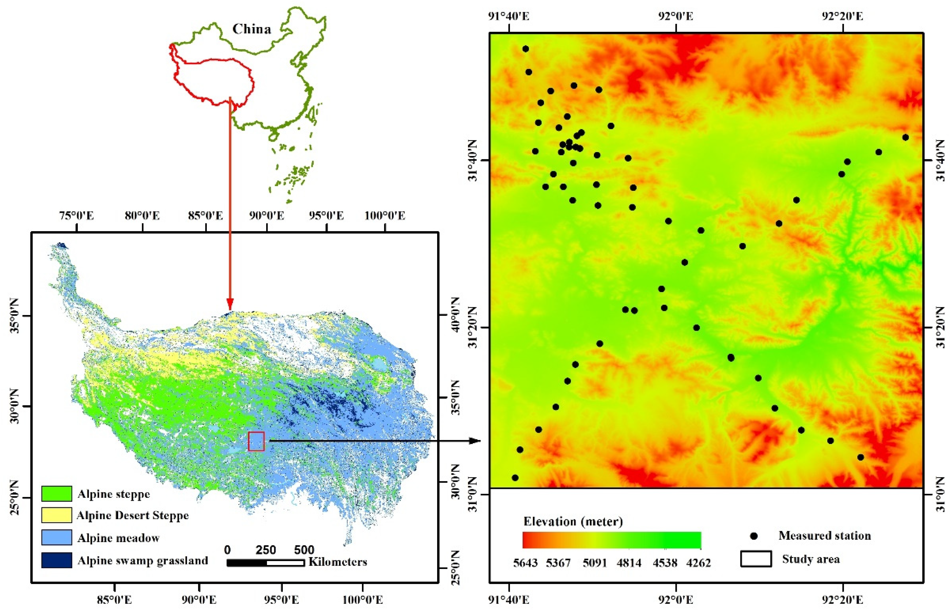
2.1. Study Area

The Tibetan Plateau has a unique geographical location, geological structure, climatic characteristics, and rich ecological resources, all of which make it important to the global ecosystem. The soil moisture in this area is an important reference value for the study of the global water cycle and precipitation mechanisms. In this study, the Naqu region in the hinterland of the Tibetan Plateau, located in the northern part of Tibet, was used as the research area to carry out soil moisture inversion research (Figure 1). The average elevation is around 4500 m in this area, but the terrain is relatively flat and has small undulations, and the main vegetation cover type is high-altitude pasture. The climate is characterized by extreme cold, lack of oxygen, little rain, and regular winds; the annual precipitation is about 380 mm [48]. The climate is dry and the temperature is low in November through March; then, it is relatively warm and the vegetation grows vigorously from May to September. During this period, the surface cover is dominated by alpine meadows and natural grasslands. Due to the special climatic conditions, the soil moisture has great spatial variability in the study area [49].

2.2. Research Data

This paper used L1 slant distance single look complex (SLC) Sentinel-1 data, the acquisition mode was interferometric wide swath (IW), the spatial resolution was 5 m × 20 m, the revisit period was 2 days, and the polarization mode was VV polarized. Equipped with a C-band synthetic aperture radar instrument with a working frequency of 5.4 GHz, it provided radar series data all-time and all-weather. The data came from the Sentinel Satellite Data Service Center of the European Space Agency (ESA) (https://scihub.copernicus.eu/, accessed on 1 November 2021). After preprocessing the Sentinel-1 data, for example, orbit correction, thermal noise removal, radiometric calibration, geocoding, and cropping, the backscatter coefficients were extracted and converted into decibels. Landsat-8 OLI image data, with a spatial resolution of 30 m, a synthetic image resolution of 15 m, and a time resolution of 16 days came from the geospatial data cloud (http://www.gscloud.cn, accessed on 1 November 2021). DEM data, with a spatial resolution of 12.5 m, was used to extract elevation information, which came from NASA’s official website (https://search.asf.alaska.edu/, accessed on 1 November 2021). There were 60 effective ground-measured soil moisture sites in the study area, which were continuously observed from August 2010 to December 2016. In this paper, the daily average observation value of soil water content at a depth of 0–10 cm from January 2015 to December 2016 was selected as the real value for model training and verification. The distribution of measured sites is shown in Figure 1. The data came from the International Soil Moisture Network (ISMN).

2.3. Methodology

2.3.1. Vegetation Water Content

In this study, we used Chan’s method to calculate vegetation water content (VWC) [46]. Scholars such as Wang used this model to calculate the vegetation water content and optimize the parameters for the Naqu area [50]. The specific method is shown in Equation (1):

$$\mathrm{vwc}=\left(1.9134NDV{I}^2-0.3215NDVI\right)+st·\frac{NDV{I}_{max}-NDV{I}_{min}}{1-NDV{I}_{min}}$$

(1)

where VWC is the vegetation water content (kg/m²) and NDVI_max and NDVI_min represent the maximum and minimum values of the normalized difference vegetation index (NDVI). st represents the product of the average vegetation height and the ratio of the stem area to stem leaf area, and represents the estimated value of the stem moisture peak. The default value of the dry factor is set to 1.5 when the vegetation type is grass [51]. The default value may be higher because the vegetation is high-altitude pasture in the study area, which is a low-coverage vegetation type. So the factor was adjusted to 0.3 after learning from other research about this area [52].

2.3.2. Calculation of the Bare Soil Backscatter Coefficient by the Water Cloud Model

It is difficult for the coverage of surface vegetation to reach 100%, and the information obtained from only optical or radar images is simultaneously affected by vegetation and soil. Therefore, combining microwave and optical remote sensing data and using the water cloud model to eliminate the influence of vegetation on backscatter helped to improve the accuracy of the soil moisture retrieval results. Vegetation water content affects the backscatter and attenuation factors of vegetation. The vegetation water content obtained according to Equation (1) was used as a water cloud model parameter to eliminate the influence of vegetation cover on backscatter. The model is expressed as Equations (2)–(4):

$${\sigma °}_{total}={\sigma °}_{veg}+{\tau }^2{\sigma °}_{soil}$$

(2)

$${\sigma °}_{veg}=\left(1-{\tau }^2\right)A·VWC·cos\theta$$

(3)

$${\tau }^2=exp\left(\frac{-2B·VWC}{cos\theta }\right)$$

(4)

We calculated the bare soil backscatter coefficient based on the water cloud model, the equation is as Equation (5):

$${\sigma °}_{soil}=\frac{{\sigma °}_{total}-{\sigma °}_{veg}}{{\tau }^2}$$

(5)

where θ is the incident angle of the sensor, σ° is the backscatter coefficient, ${\sigma °}_{veg}$ represents the vegetation backscatter coefficient, ${\sigma °}_{soil}$ represents the soil backscatter coefficient, ${\tau }^2$ is the double-layer attenuation factor of microwave penetration through the vegetation layer, and A and B are two parameters dependent on vegetation type. Studies have shown that parameter A is less sensitive to the backscatter coefficient, while the backscatter coefficient decreases along with the increase in parameter B, and the amplitude of change increases with the increase in VWC. Referring to the B value in

Table 1. The vegetation parameters of the water cloud model [25].

Parameters	All Vegetation	Grazing Land	Winter Wheat	Grassland
A	0.0012	0.0009	0.0018	0.0014
B	0.0910	0.0320	0.1380	0.0840

, we experimented with 0.01 as the interval between 0.03 and 0.14. When B was 0.05, the soil moisture inversion results were closest to the measured soil moisture value [53].

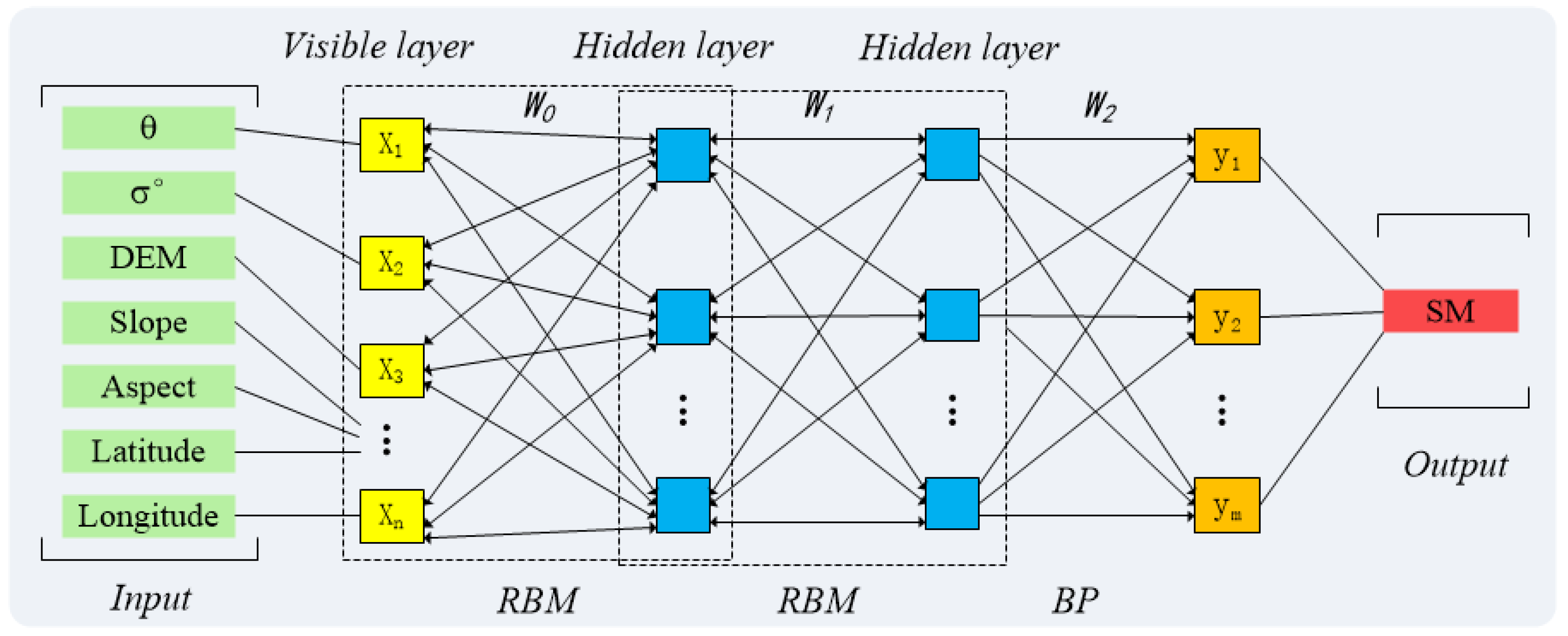
2.3.3. Deep Belief Network Soil Moisture Retrieval Model

The deep belief network (DBN) model was proposed by Hinton in 2006. It is one of the typical deep learning models. DBN is composed of multiple restricted Boltzmann machine (RBM) layers and a backpropagation (BP) layer. The structure is shown in Figure 2. The RBM consists of a visible layer and a hidden layer, where the hidden layer of the previous RBM is the visible layer of the next RBM. Moving from the visible layer (v) to the hidden layer (h) is represented by Equation (6):

$$h_i^1=\{\begin{array}{c}1,f\left(w_{0,i}X+b_i\right)\ge \mu \\ 0,f\left(w_{0,i}X+b_i\right)<\mu \end{array} \mu ~U\left(0,1\right)$$

(6)

where i and b_i refer to the number of the ith neuron and the bias, respectively. f represents the ReLu function used for neuron mapping between the neural network layers. Its function is to improve the nonlinear modeling ability of the model and to better excavate the deep information between the input feature values, and the same is used to calculate the visible layer from the hidden layer. The weights were updated in the nth as Equation (7):

$$W_0^{n+1}=W_0^n+\epsilon ({(h_1^1)}^{T}X-{(h_2^1)}^T{V}_1)$$

(7)

The bare soil backscatter coefficient, topographic factors, and soil moisture have multiple and complex mapping relationships. DBN has the characteristic of quickly establishing mapping relationships from complex relationships. Using DBN to retrieve soil moisture has great potential. Model training included the pretraining by RBM and the process of error backpropagation by the BP neural network to fine-tune network weights and biases. We used an unsupervised method to train each layer of RBM, input the preprocessed sample data into the visible layer of RBM, passed the data to the hidden layer through the excitation function, and used the Gibbs sampling ratio divergence algorithm to update the weights and deviations value. In the BP neural network, the SmoothL1 function was used as the loss function; it prevented the gradient explosion caused by the running of the model compared with the mean square error function.

The deep belief network soil moisture inversion model was based on the bare soil backscatter coefficient calculated by the water cloud model, combined with incident angle, terrain elevation, latitude, and longitude as input data, and the measured site data were used as label data to invert soil moisture. The model is expressed as Equation (8):

$$SM=f\left(\theta ,\sigma {°}_{soil},DEM,Slope,Aspect\right)$$

(8)

where f() refers to the prediction function and θ is the angle of incidence. $\sigma {°}_{soil}$ refers to the bare soil backscatter coefficient, which was mainly used to obtain ground soil moisture information; DEM, slope, and aspect represent the effects of terrain factors.

2.3.4. Accuracy Evaluation

This paper used the Pearson correlation coefficient (R), root mean square error (RMSE), bias, degree of fit (R²), average absolute percentage error (MAPE), and the Theil nequality coefficient (TIC) to assess the accuracy of the DBN soil moisture inversion results. For a detailed description of each accuracy index, refer to references [54,55].

The ten-fold cross-validation technique, proposed by Rodriguez in 2010 [56], was used to test the stability and generalization ability of the DBN soil moisture inversion model in this study. This technique is usually used to evaluate the performance of machine learning models on limited data samples [57]. First, all the sample data were shuffled and randomly divided into ten groups. One group was selected as the test data set, and the other nine groups were used as the training data set to fit the model. Then we trained the model in turn, repeating the fitting model on the training set. Finally, the average of ten rounds of accuracy evaluation was taken to represent the accuracy and stability of the prediction model.

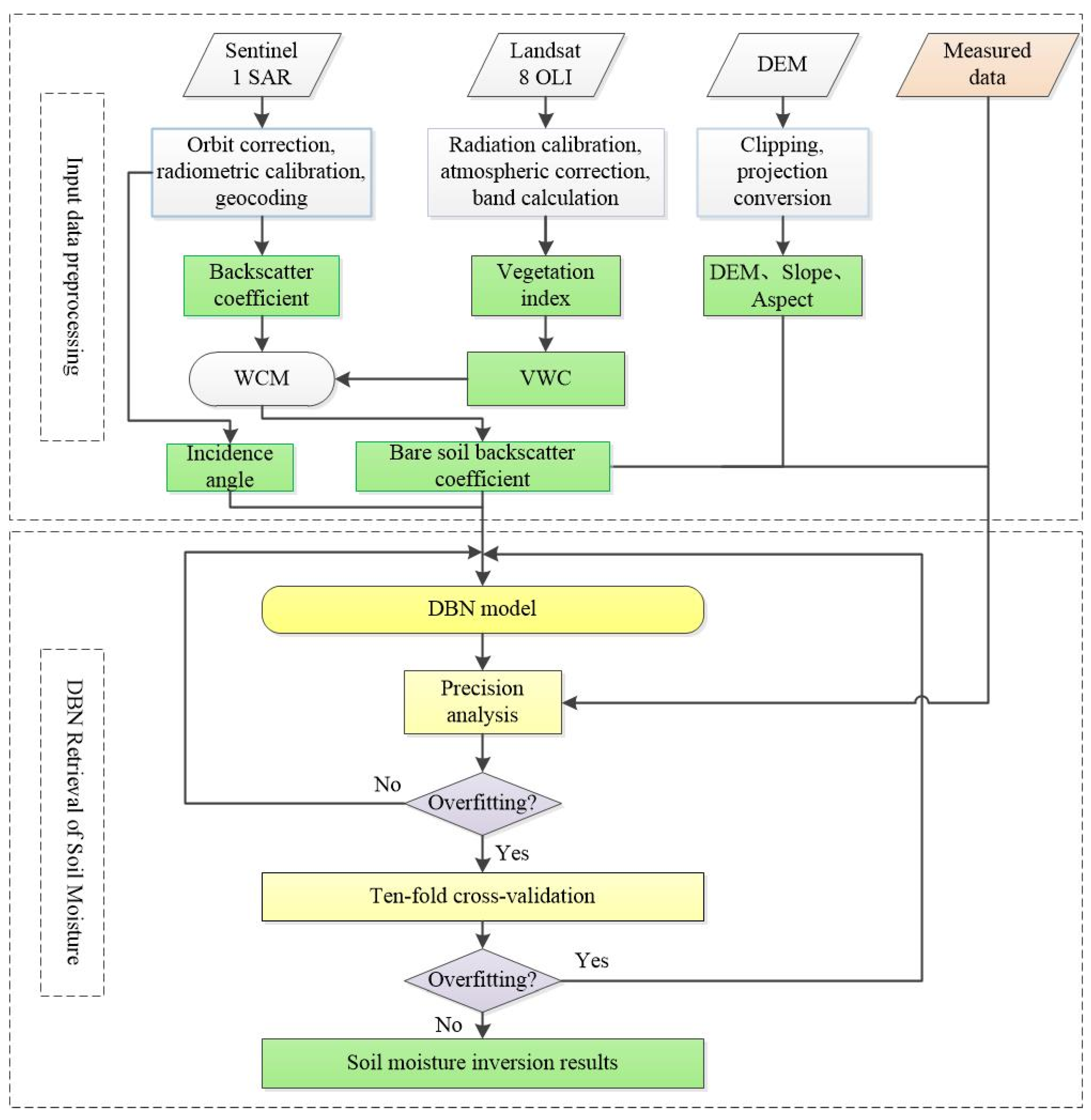
2.3.5. Technical Process

The workflow is shown in Figure 3.

• After preprocessing the Sentinel-1 data, extract the backscatter coefficient and incident angle information.
• Obtain the NDVI after preprocessing Landsat-8 OLI data, and calculate VWC according to Equation (1).
• Combine the backscatter coefficient and VWC and calculate the bare soil backscatter coefficient according to the water cloud model to eliminate the vegetation cover effect on the backscatter.

Use the incident angle, bare soil backscatter coefficient, terrain elevation, latitude, and longitude information obtained in the previous steps as the DBN model input data, and use the measured data as the label data to establish the DBN soil moisture inversion model. Use the accuracy evaluation index to evaluate the model accuracy and use the ten-fold cross-validation technique to evaluate the model stability.

3. Results and Analysis

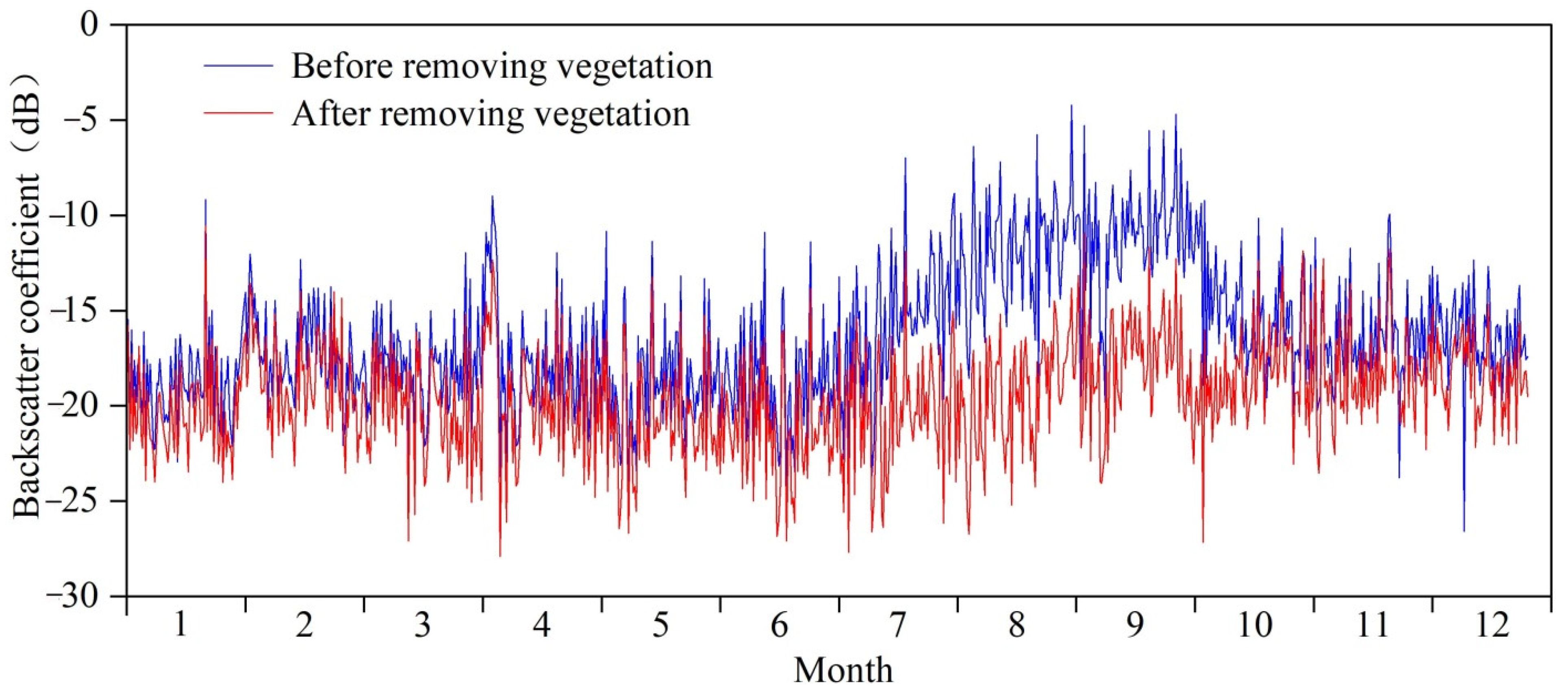
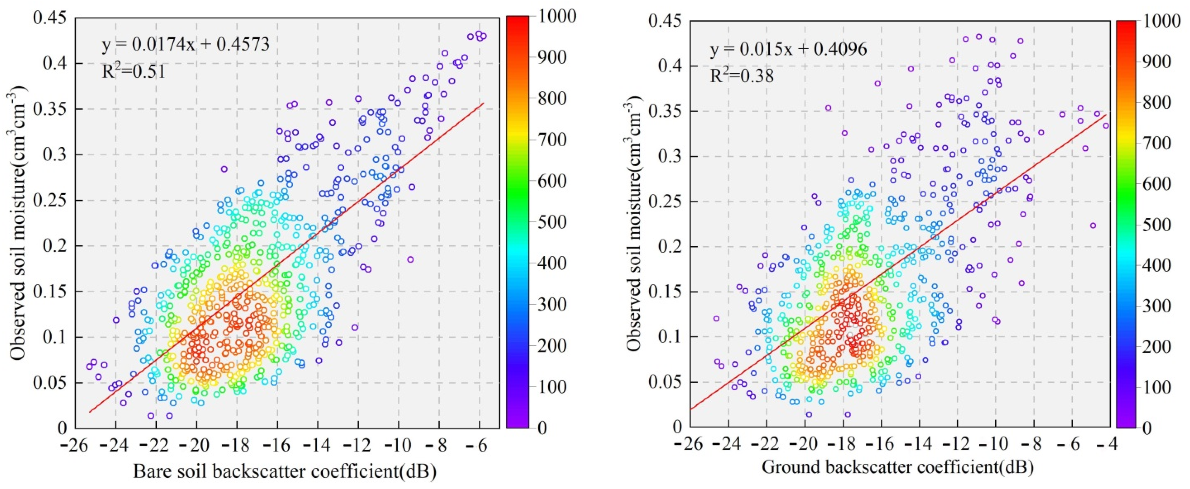
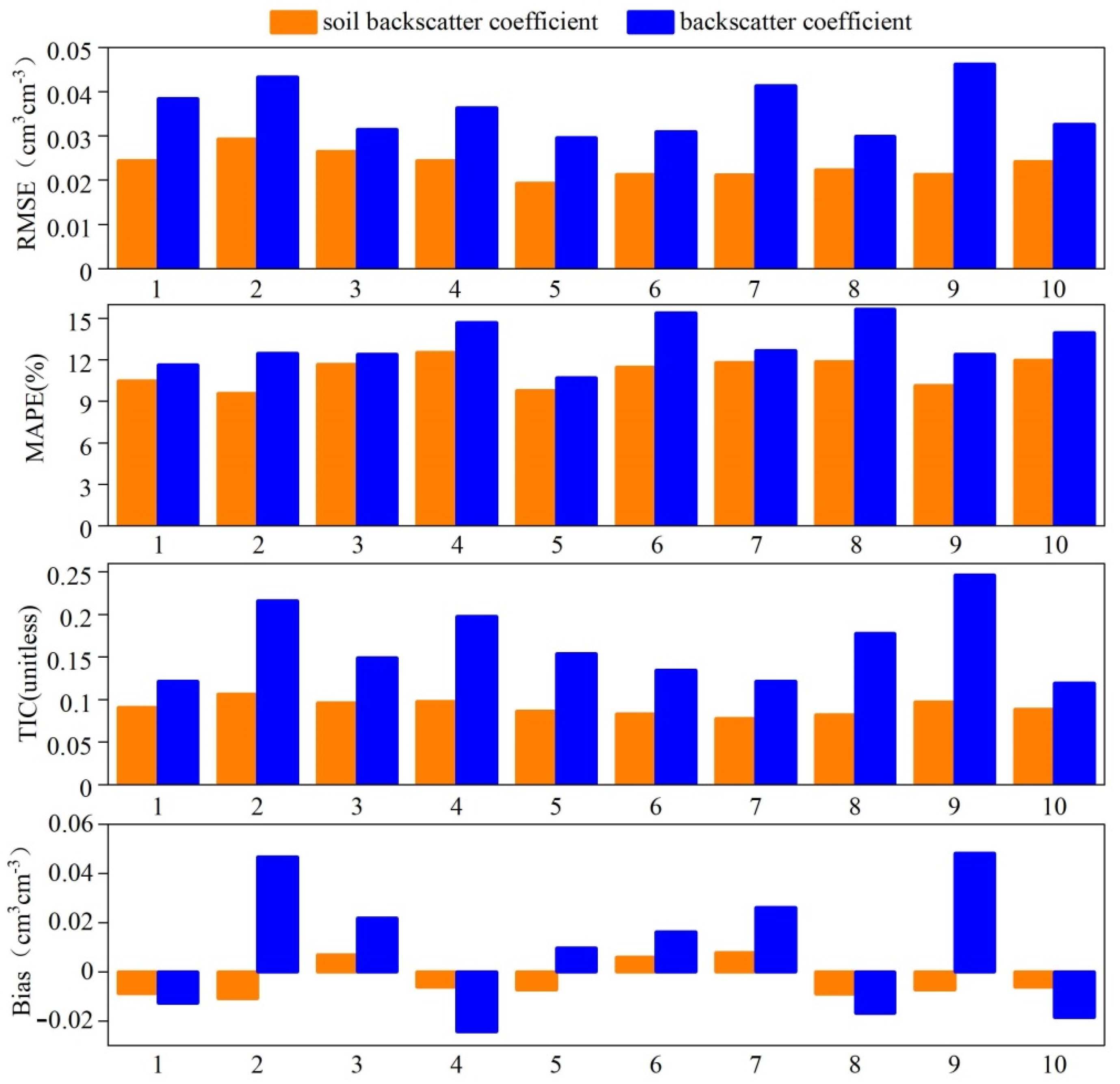
3.1. Calculation of the Bare Soil Backscatter Coefficient and Analysis of Its Correlation with Soil Moisture

According to the water cloud model, the backscatter coefficient values, from before and after the vegetation effect was eliminated, were obtained for the Naqu area in 2016. The results are shown in Figure 4. The results showed that the vegetation coverage effect increased the backscatter value. The vegetation effect on the backscatter was more significant during the lush vegetation period from July to September, and the backscatter coefficient increased significantly. The backscatter coefficient average value was −16.27 before removing vegetation, the bare soil backscatter coefficient average value was −19.51 after removing vegetation, and the average value of the backscatter coefficient from July to September before and after eliminating the vegetation was −12.04 and −18.81, respectively. The bare soil backscatter value decreased overall after eliminating the vegetation cover effect, but the reduction was different in different time periods. The main reason is that the vegetation varies with the climate and seasons in different periods. The small gap period was the period of cold and dry air when vegetation was sparse and withered, during which the ground backscatter value was close to the bare soil backscatter, so the difference was small before and after vegetation was eliminated. However, the difference was greater in the period of vigorous vegetation growth, and the vegetation contribution to the backscatter was greater; hence, the backscatter coefficients before and after eliminating the vegetation cover effect were further apart.

The correlation analysis between the backscatter coefficient before and after removing the vegetation effects and the soil moisture measured value is shown in Figure 5. The results showed that the correlation between the soil backscatter coefficient and soil moisture was significantly improved after eliminating the vegetation effect, and the R² increased from 0.38 to 0.51. The scattered points of bare soil backscatter coefficient and soil moisture were more concentrated, and the aggregation effect was significantly increased in soil moisture high-value areas. The vegetation elimination significantly improved the fit between the backscatter value and soil moisture. Vegetation increased the contribution of backscatter to the ground in the soil moisture high-value areas, which influenced the mapping relationship between soil backscatter and soil moisture. Correlation analysis fully showed that vegetation cover was an important factor affecting the backscatter coefficient inversion of soil moisture. Eliminating the vegetation cover effect will further clarify the relationship between soil moisture and soil backscatter, and help improve the soil moisture retrieval accuracy.

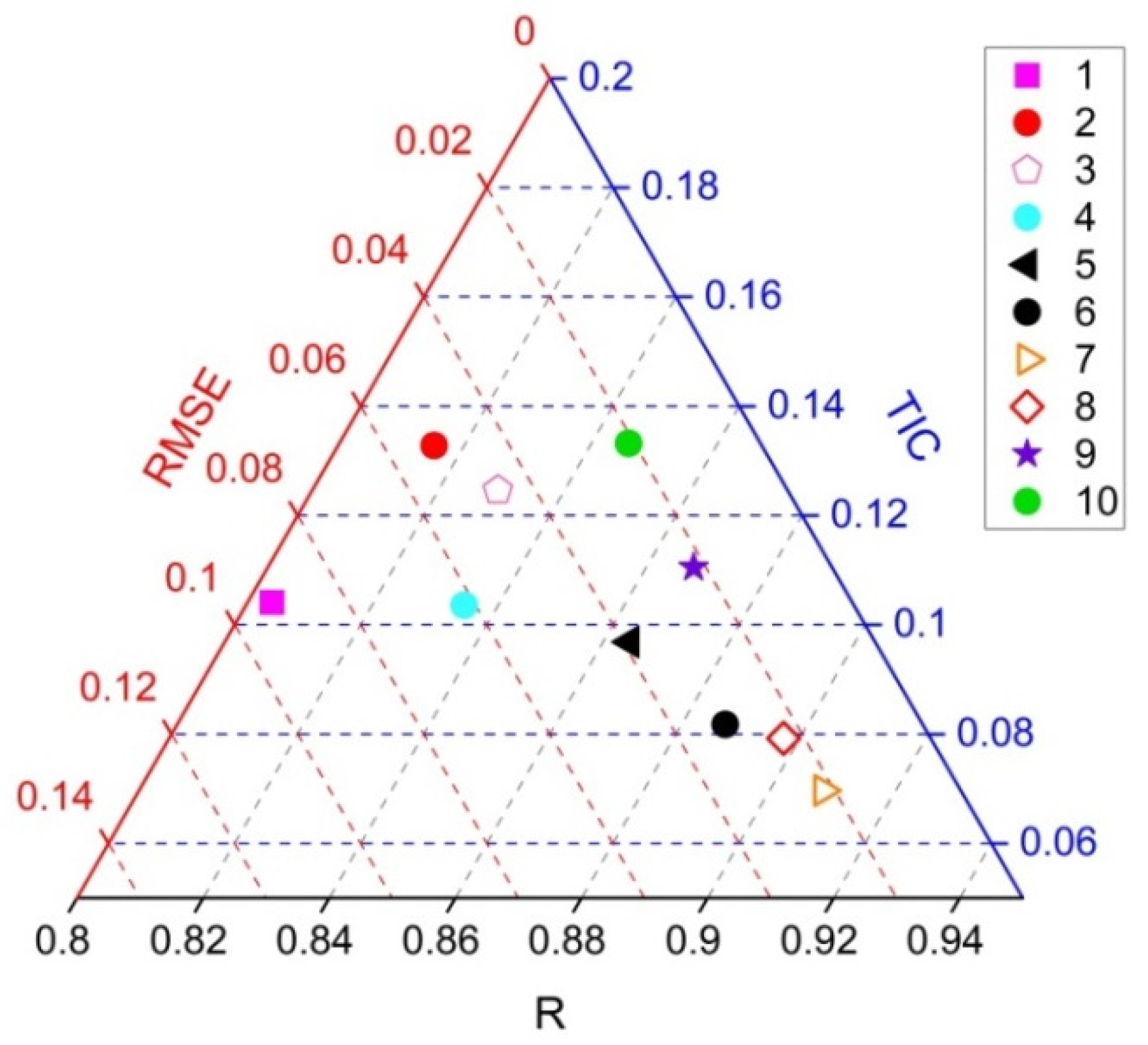
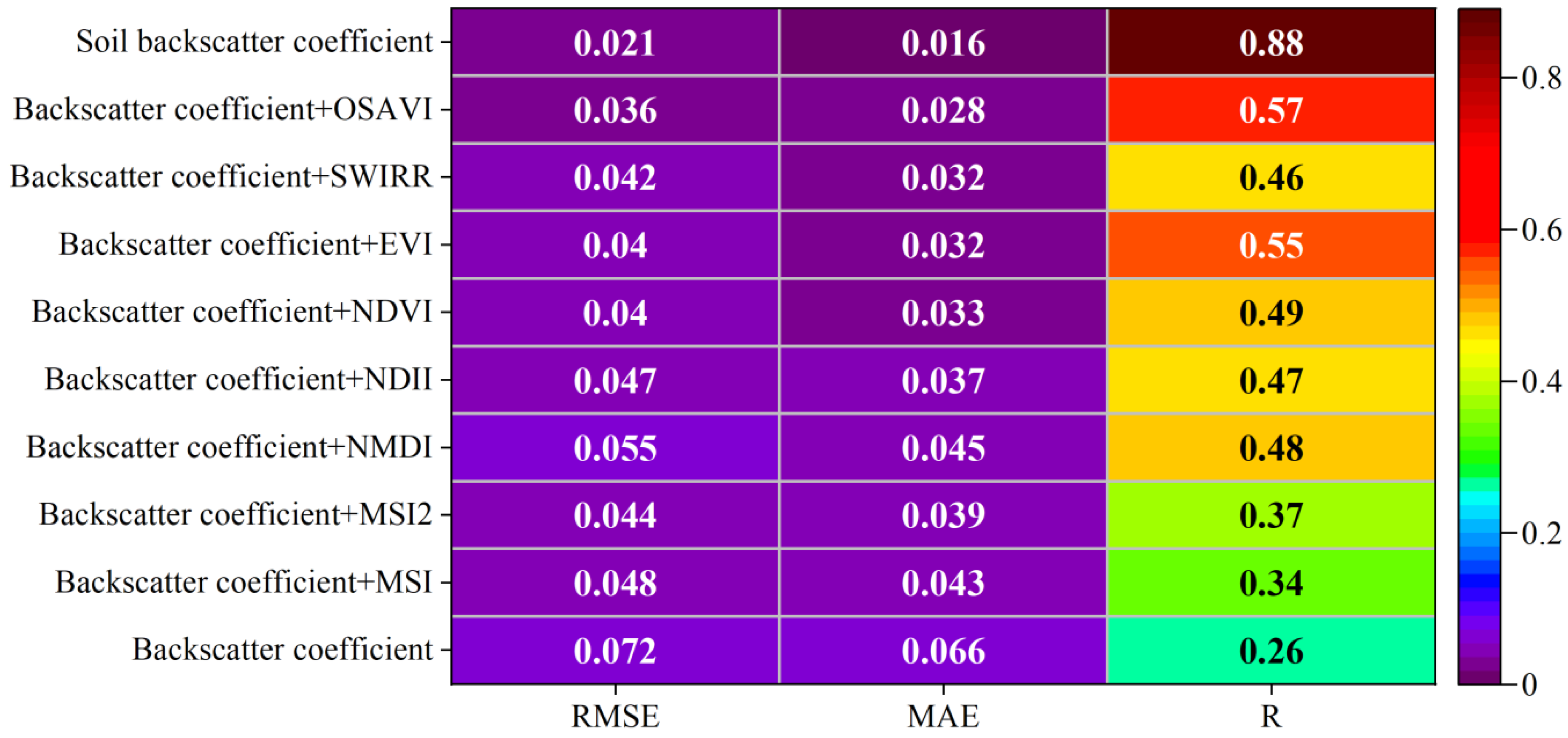
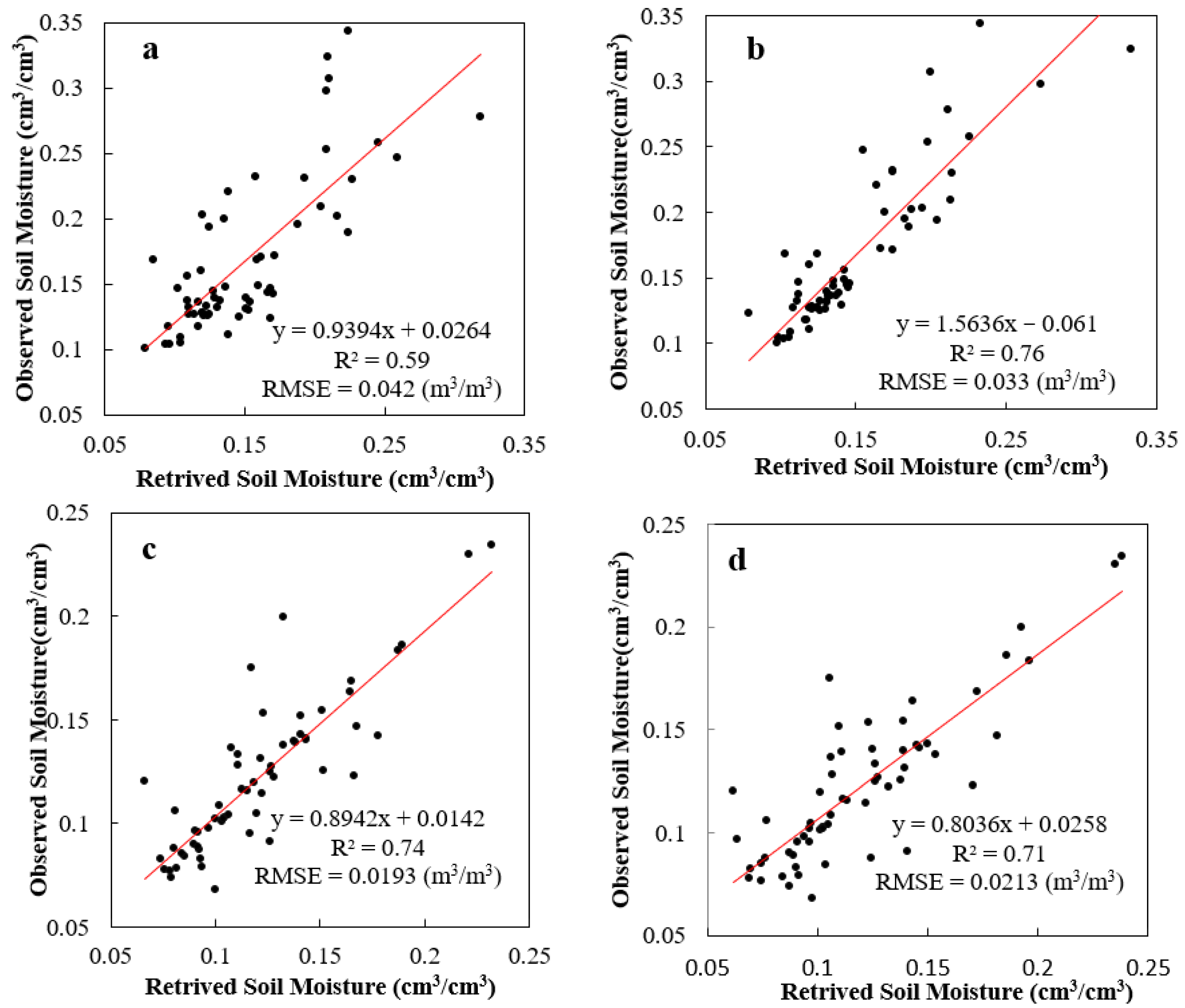
3.2. Accuracy Assessment of Soil Moisture Inversion by Deep Belief Network Model

The bare soil backscatter coefficient, radar incident angle, DEM, slope, and aspect were used as training data, and the measured soil moisture data were used as label data to establish a DBN soil moisture inversion model. Through the experiments, we found that compared to the Sigmoid function, the ReLu function as the activation function was less likely to cause the gradient vanishing during backpropagation, and the convergence speed was better. The ReLu function gave some neurons a value of zero, which was helpful to prevent the overfitting phenomenon. We began to use MSE as the loss function, but because it is a square operation, the difference was amplified when the soil moisture real value was significantly different from the predicted value, and the error would easily cause gradient explosion when the error was backpropagated. Therefore, we used the SmoothL1 loss function to effectively prevent the gradient explosion when the model was running. In addition, the number of RBM layers had a significant impact on the prediction result in the model; they were adjusted to determine the optimal accuracy of the prediction result (Figure 6). We observed the changes in R² and bias by increasing the number of RBM; R² represented the fitting performance of the model predicted value, and bias was the degree of deviation between the predicted value and the real value. The results showed that the overall change of R² was small, between 0.6 and 0.8, but the bias of the RBM prediction results was more than 0.015 before the third layer, and the deviation was large. After the fourth layer, the deviation was between −0.005 and 0.005, and the deviation changes tended to stabilize. When the RBM was seven layers, R² was 0.78 at the maximum value, and the deviation value was also small at 0.007, so the deep belief network soil moisture inversion model performance was most precise when the RBM was set to seven layers.

The model was tested and evaluated by three error evaluation indicators: the correlation coefficient (R), inequality coefficient (TIC), and root mean square error (RMSE) (Figure 7). The results showed that the comprehensive prediction performance of the model was reduced when there were too many or too few RBM layers. The R-value between the model predicted result and the measured value gradually increased along with the increase in RBM layers, and the TIC and RMSE gradually decreased. The accuracy tended to stabilize when the RBM reached six to eight layers. The RMSE value changed less and the error was minimized between the predicted value and the real value when the RBM was increased to nine layers, but the R-value was significantly reduced. The R-value was further reduced when the RBM was 10 layers to 0.06 and the TIC increased, which showed that the prediction results accuracy had decreased. Through the analysis of the accuracy changes of different RBM layer models, it was concluded that the model prediction result had the best accuracy when the RBM was seven layers. Therefore, this study selected the DBN model with seven RBM layers as the soil moisture inversion model.

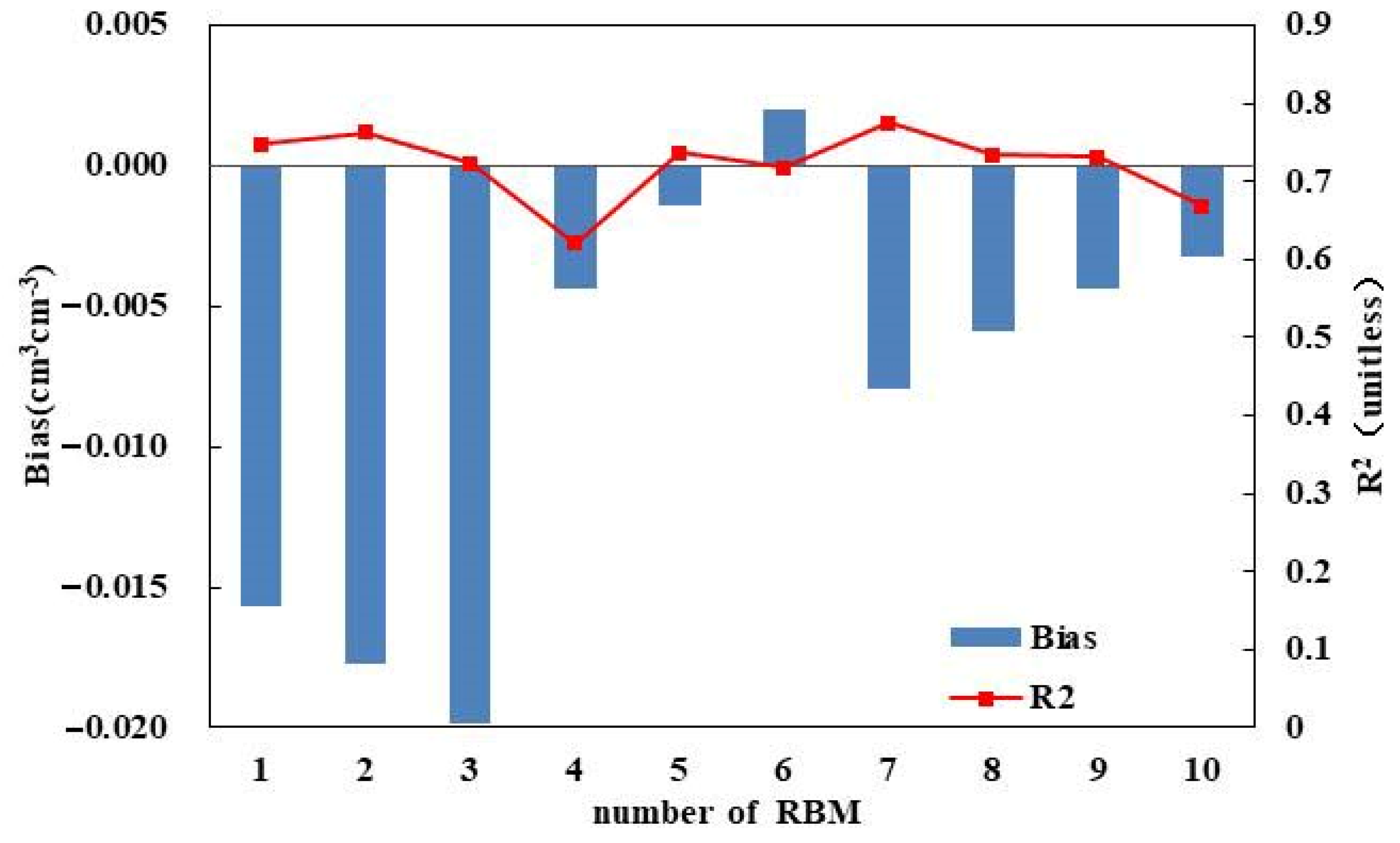
3.3. Ten-Fold Cross-Validation

Ten-fold cross-validation showed that multiple error evaluation indicators tended to be stable and have small fluctuations (Figure 8); it showed that the model performance was relatively stable after training, and there was no error fluctuation with data changes. Compared with the ground backscatter coefficient, the inversion result accuracy was improved and more stable when the bare soil backscatter coefficient was used as the training data. Therefore, human intervention to increase the correlation between input data and prediction results before creating the DBN network model improved the performance of the DBN soil moisture retrieval model.

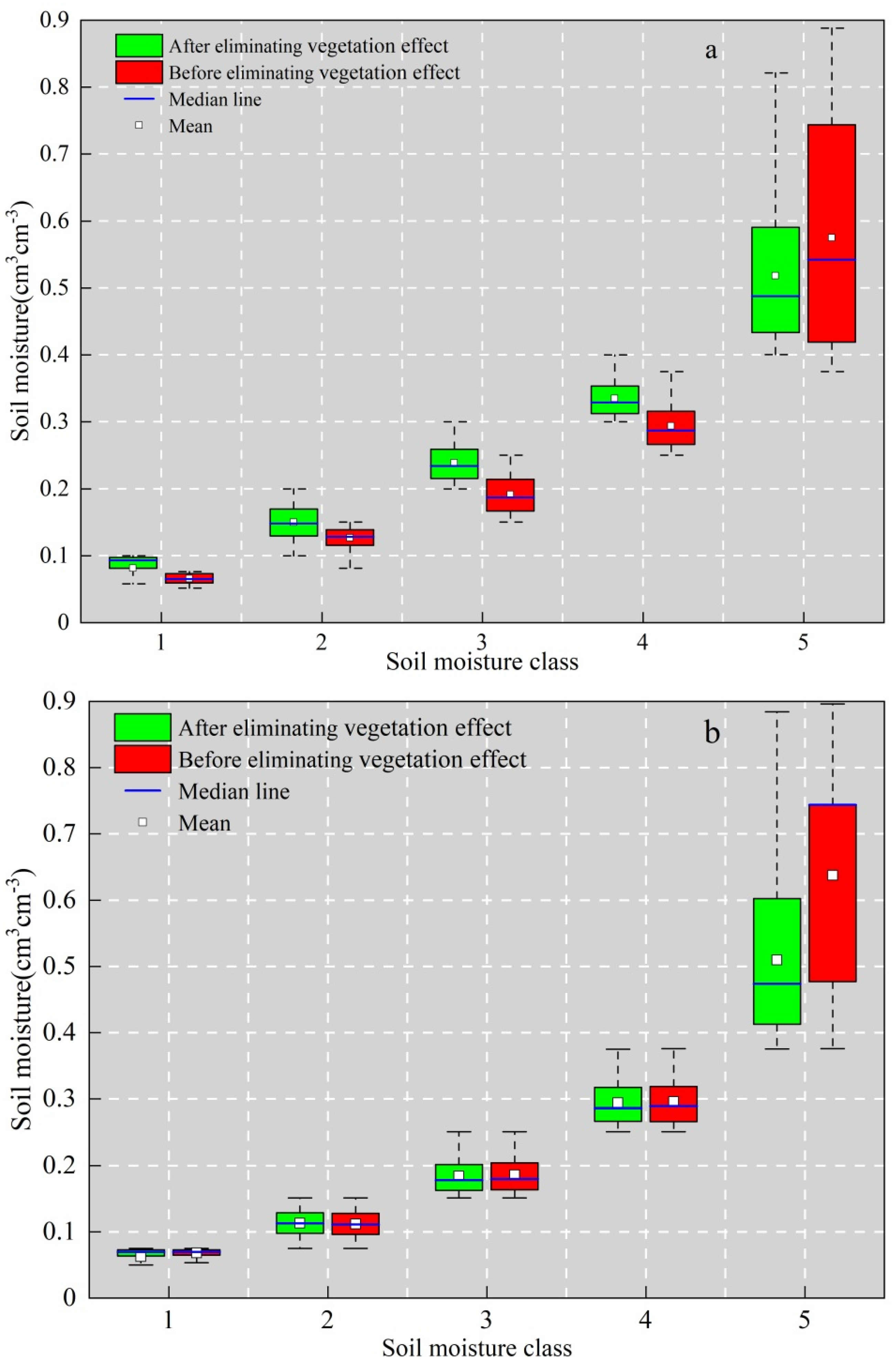
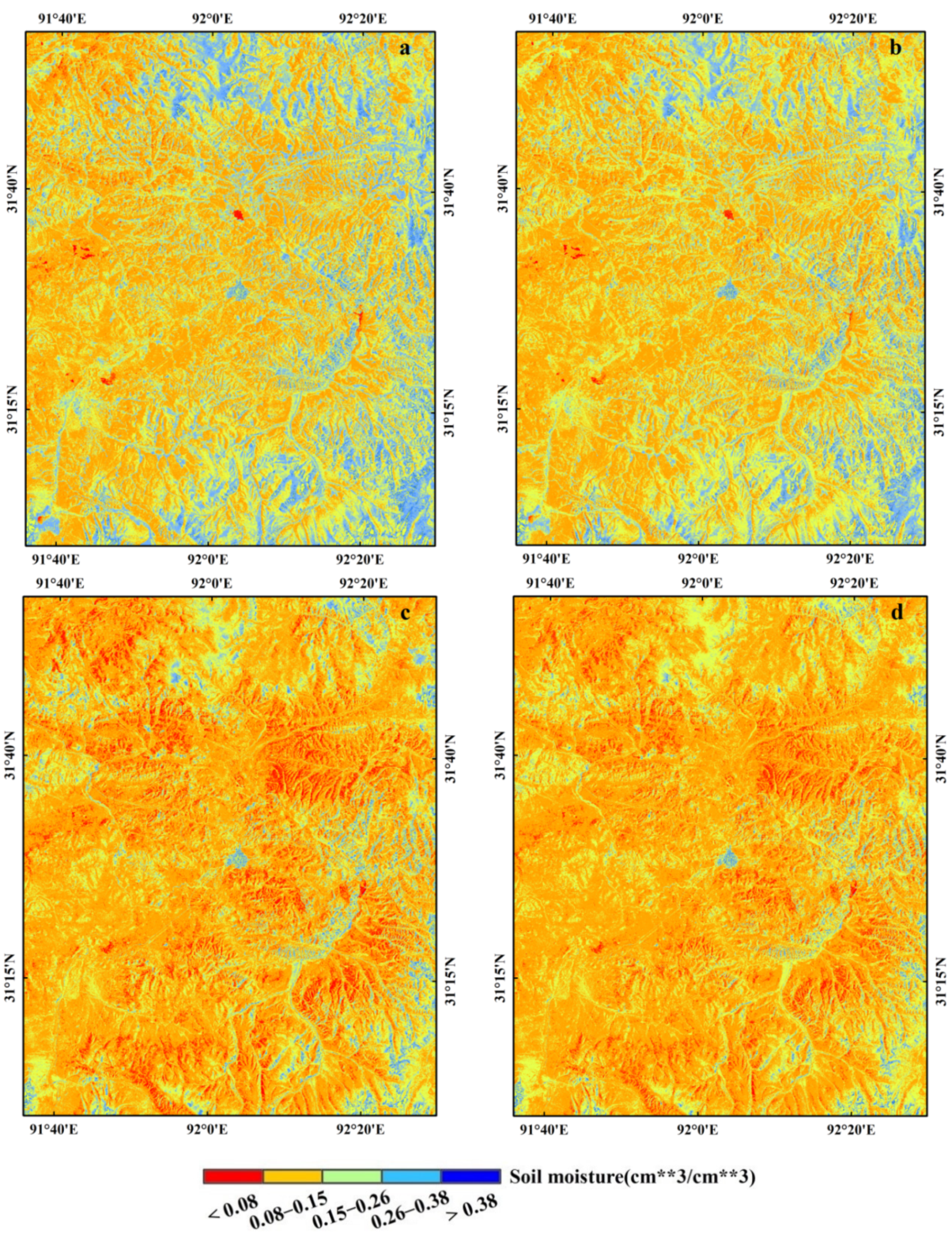
3.4. Analysis of Soil Moisture Inversion Results

The DBN soil moisture inversion model was used to predict the soil moisture in the Naqu area of the Tibetan Plateau (Figure 9). To train the soil moisture inversion model, the backscatter coefficient before and after removing the vegetation cover influence and the angle of incidence and terrain factor were used, and we analyzed the vegetation coverage effect on the soil moisture inversion results’ accuracy. We retrieved one phase of soil moisture data in July when the vegetation coverage was high and another in December when the vegetation coverage was low, respectively, and analyzed the differences in the inversion results before and after the removal of vegetation coverage. The results showed that the soil moisture prediction values were different before and after the elimination of vegetation cover in July. Vegetation coverage made the soil moisture prediction higher especially in the eastern soil moisture high-value areas. The vegetation withered and the ground surface was bare in December, so the ground backscatter basically represented the bare soil backscatter status during that period. Therefore, the difference was small in the soil moisture inversion results before and after the removal of vegetation cover, and the soil moisture value decreased overall in December. The soil moisture overall spatial distribution pattern was high in the east and low in the central and western regions in the study area. Compared with the elevation information in Figure 1, most of the high soil moisture areas were in high-altitude areas, and these areas had more vegetation coverage, less evapotranspiration, and easy access to precipitation replenishment, so the ground soil moisture was relatively high [23]. The soil moisture was lower in central and western regions because most areas were bare soil, where evapotranspiration was stronger and the vegetation coverage was lower. The spatial distribution comparative analysis shows that the DBN soil moisture inversion model prediction results based on the bare soil backscatter coefficient were more reliable after removing the vegetation cover.

The measured data were used to further verify the soil moisture results of the model based on the backscatter coefficient and the bare soil backscatter coefficient. The fitted scatter plot is shown in Figure 10. The inversion result fitting coefficient based on the backscatter coefficient (R² = 0.59, p < 0.01) was smaller than the inversion result fitting coefficient based on the bare soil backscatter coefficient (R² = 0.76, p < 0.01), and the RMSE decreased from 0.042 to 0.033, which showed that the vegetation cover caused the soil moisture inversion results to deviate in June. The inversion results’ fitting coefficients were (R² = 0.74, p < 0.01) and (R² = 0.71, p < 0.01) based on the ground backscatter coefficient and bare soil backscatter coefficient, and the RMSE values were 0.019 and 0.021, respectively; there was little difference in the soil moisture inversion results accuracy before and after the vegetation cover was eliminated in December. The comparative accuracy analysis of the two phases’ inversion results shows that the vegetation coverage reduced the soil moisture inversion accuracy, and the influence was more significant during the vigorous vegetation growth period.

The soil moisture inversion results’ classification statistics (Figure 11) show that the effects of vegetation coverage on different degrees of soil moisture values varied. The first two levels’ average value of SM inversion results after vegetation elimination was slightly greater than the inversion value before vegetation elimination; this difference increased at the third and fourth level and the mean difference was 0.041 and 0.043, respectively. The vegetation effect somewhat underestimated the soil moisture in this area. However, the fifth level SM average value increased by 0.056 after removal of vegetation, and the third-quarter value increased significantly, indicating that vegetation coverage caused the moisture to be overestimated in high soil moisture values areas. The soil moisture statistical results from one to four levels differed slightly, and the median and average values remained about the same before and after devegetation in December. However, the fifth level’s soil moisture value had a large difference before and after devegetation, and vegetation still caused an overestimation of soil moisture. Since the high soil moisture areas are at higher altitudes, the vegetation cover is mostly shrubs, and the high coverage vegetation increases the backscatter contribution. After a comprehensive comparative analysis, it was concluded that vegetation coverage underestimated the soil moisture inversion value in soil moisture low-value areas and overestimated the soil moisture inversion value in high-value areas.

4. Discussion

Vegetation coverage has a significant effect on the soil moisture inversion of the backscatter coefficient. Based on the ground backscattering coefficient and terrain elevation factor as the basic training data, combined with different vegetation indices, the DBN soil moisture inversion model prediction results were also different. The accuracy results are shown in Figure 12. The calculation methods of each vegetation index were detailed in [58]. When only the ground backscatter and elevation factors were considered, the inversion results’ accuracy was the lowest; the correlation coefficient R was 0.26 (p < 0.05), and the RMSE value was the highest at 0.072. While the prediction accuracy was improved when the backscatter coefficient and vegetation index were combined as model training data, the accuracy difference was small when combined with different vegetation indexes, with an R average of 0.47 (p < 0.05). The inversion results’ accuracy was higher when the vegetation index was EVI and OSAVI; the R-value was 0.55 and 0.57 (p < 0.05), respectively, which was an increase of 0.1 compared to the R average. Since the EVI and OSAVI indices consider more bands and reduce the influence of the atmosphere and vegetation canopy, it effectively improved the sensitivity of vegetation information in high vegetation coverage areas; the averages of RMSE and MAE were 0.044 and 0.036, respectively, and the soil moisture inversion results’ accuracy based on different vegetation indices had little difference. The bare soil backscatter coefficient inverse soil moisture results’ accuracy was significantly improved; the R-value increased to 0.88 (p < 0.05), and the RMSE and MAE values decreased to 0.021 and 0.016, respectively. Since NDVI is easily saturated in high vegetation coverage areas, it is mainly suitable for inversion soil moisture in low vegetation coverage areas. The comparative study further proved the significant influence of vegetation coverage on the backscatter coefficient inversion soil moisture, and if the combination of backscatter coefficient and vegetation index is simply used as the input data, it is difficult to effectively improve the inversion results’ accuracy. Therefore, the water cloud model was used to eliminate the vegetation backscatter contribution from the mechanism. Then we used the bare soil backscatter coefficient as the input data for the DBN to establish the relationship with soil moisture, which enabled the neural network characteristics to perform better and significantly improved the backscatter coefficient inversion soil moisture accuracy.

In the Naqu area of the Tibetan Plateau, many scholars have used different models for soil moisture inversion research, for example, Yang combined a vegetation water cloud model and cost distance function to estimate soil moisture [53]; the R² was 0.46 and RMSE was 0.08 in the accuracy analysis. Wang used the semiempirical Oh model to estimate the surface roughness parameters to improve the water cloud model before soil moisture inversion [51] and obtained a higher accuracy of soil moisture inversion results (R = 0.89 and RMSE = 0.058). However, the research model was more complicated and needed a large number of measured parameters to improve and calibrate the model. In most studies, the number of measured values was limited and had a greater impact on the results. Our study obtained a good inversion result (R = 0.88, RMSE = 0.021), by eliminating the vegetation cover influence on the backscatter. Combining this with the DBN model, the prediction result accuracy was further improved compared to the cost distance function prediction result. The mapping relationship was established between bare soil backscatter and soil moisture, which reduced the limitation of the measured parameters on the inversion results’ accuracy.

5. Conclusions

By combining the WCM and the DBN model and using Sentinel-1 synthetic aperture radar and Landsat-8 optical data to retrieve soil moisture in the Naqu area of the Tibetan Plateau, this paper draws the following main conclusions:

Using the ground backscatter coefficient and VWC, calculated according to NDVI, based on the water cloud model to eliminate the vegetation cover effect on the backscatter, and obtaining the bare soil backscatter coefficient was successful. The bare soil backscatter coefficients were combined with the incident angle and terrain factors as training data, and the ground-measured soil moisture data were used as the label data to establish a DBN soil moisture inversion model. The mapping relationship between soil backscatter and soil moisture was clarified. Studies have shown that vegetation has a great effect on ground backscatter. There are significant differences in backscatter values before and after removing vegetation cover. The bare soil backscatter coefficient average value compared to the ground backscatter coefficient average value was lower by 3.23 dB. Vegetation has a significant effect on backscatter, especially during high vegetation coverage periods. By comparing and analyzing the soil moisture inversion results before and after the removal of vegetation coverage in different vegetation coverage periods, it was concluded that the soil moisture accuracy based on the bare soil backscatter coefficient (R² = 0.50) was higher than that based on the ground backscatter coefficient (R² = 0.38), and more in line with the ground-measured data.

In the DBN soil moisture inversion model, choosing ReLu as the activation function did not cause the gradient to disappear, the convergence speed was also better, and it prevented the model from overfitting. In the model, SmoothL1 was used as the loss function, which effectively prevented the gradient explosion that can occur when the difference between the true value and the predicted value is large in the backpropagation process. Setting different RBM layers in the DBN neural network had a significant impact on the model performance. The experiment showed that the prediction result accuracy was best when the bare soil backscatter was used as the main input data to invert the soil moisture and the neural network had seven layers. In addition, the prediction results’ accuracy had less volatility, and the model was more stable.

The comparative analysis of soil moisture prediction results found that the DBN soil moisture inversion model used Sentinel-1 data to achieve good results in soil moisture inversion. Soil moisture was overestimated in high vegetation coverage areas and underestimated in low vegetation coverage areas when the model was based on ground backscatter inversion, and between the backscatter coefficient and vegetation index simple combination in the DBN model, it was difficult to improve the soil moisture inversion results’ accuracy. However, when the bare soil backscatter coefficient was used as training data after the physical model eliminated the vegetation coverage effect, its inversion results were consistent with the actual surface conditions, and the spatial details were expressed more clearly.

References

- Seneviratne, S.I.; Corti, T.; Davin, E.L.; Hirschi, M.; Jaeger, E.B.; Lehner, I.; Orlowsky, B.; Teuling, A.J. Investigating soil moisture–climate interactions in a changing climate: A review. Earth Sci. Rev. 2010, 99, 125–161. [Google Scholar] [CrossRef]
- Pangaluru, K.; Velicogna, I.; Geruo, A.; Mohajerani, Y.; Ciracì, E.; Cpepa, S.; Basha, G.; Rao, S. Soil moisture variability in India: Relationship with landsurface atmospheric fields using Maximum Covariance Analysis. Remote Sens. 2019, 11, 335. [Google Scholar] [CrossRef] [Green Version]
- Peng, J.; Loew, A.; Merlin, O.; Verhoest, N.E.C. A review of spatial downscaling of satellite remotely sensed soil moisture. Rev. Geophys. 2017, 55, 341–366. [Google Scholar] [CrossRef]
- McColl, K.A.; Alemohammad, S.H.; Akbar, R.; Konings, A.G.; Yueh, S.; Entekhabi, D. The global distribution and dynamics of surface soil moisture. Nat. Geosci. 2017, 10, 100–104. [Google Scholar] [CrossRef]
- Rossini, P.R.; Ciampitti, I.A.; Hefley, T.; Patrignani, A. A soil moisture-based framework for guiding the number and location of soil moisture sensors in agricultural fields. Vadose Zone J. 2021, e20159. [Google Scholar] [CrossRef]
- Rosenzweig, C.; Tubiello, F.N.; Goldberg, R.; Mills, E.; Bloomfield, J. Increased crop damage in the US from excess precipita-tion under climate change. Glob. Environ. Chang. 2002, 12, 197–202. [Google Scholar] [CrossRef] [Green Version]
- Berardi, M.; Difonzo, F.V. Strong solutions for Richards’ equation with Cauchy conditions and constant pressure gradient. Environ. Fluid Mech. 2020, 20, 165–174. [Google Scholar] [CrossRef]
- Albrieu, J.L.B.; Reginato, J.C.; Tarzia, D.A. Modeling water uptake by a root system growing in a fixed soil volume. Appl. Math. Model. 2015, 39, 3434–3447. [Google Scholar] [CrossRef]
- Fengnan, L.; Fukumoto, Y.; Zhao, X. A linearized finite difference scheme for the Richards equation under variable-flux bounda-ry conditions. J. Sci. Comput. 2020, 83, 1–21. [Google Scholar] [CrossRef]
- Keshavarz, M.R.; Vazifedoust, M.; Alizadeh, A. Drought monitoring using a Soil Wetness Deficit Index (SWDI) derived from MODIS satellite data. Agric. Water Manag. 2014, 132, 37–45. [Google Scholar] [CrossRef]
- Jin, R.; Li, X.; Liu, S.M. Understanding the Heterogeneity of Soil Moisture and Evapotranspiration Using Multiscale Observa-tions From Satellites, Airborne Sensors, and a GroundBased Observation Matrix. IEEE Geosci. Remote Sens. Lett. 2017, 14, 21322136. [Google Scholar] [CrossRef]
- Miller, G.R.; Baldocchi, D.D.; Law, B.E. Meyers An analysis of soil moisture dynamics using multi-year data from a network of micrometeorological observation sites. Adv. Water Resour. 2007, 30, 1065–1081. [Google Scholar] [CrossRef] [Green Version]
- Qin, X.D.; Pang, Z.G.; Jiang, W.; Feng, T.; Fu, J. Progress and development trend of soil moisture microwave remote sensing retrieval method. J. Geo-Inf. Sci. 2021, 23, 1728–1742. (In Chinese) [Google Scholar] [CrossRef]
- Kumar, S.T.; Bitar, A.A.; Sekhar, M.; Zribi, M.; Bandyopadhyay, S.; Kerr, Y. MAPSM: A Spatio-Temporal Algorithm for Merg-ing Soil Moisture from Active and Passive Microwave Remote Sensing. Remote Sens. 2016, 8, 990. [Google Scholar]
- Das, N.N.; Entekhabi, D.; Njoku, E.G. An Algorithm for Merging SMAP Radiometer and Radar Data for High-Resolution Soil-Moisture Retrieval. IEEE Trans. Geosci. Remote Sens. 2011, 49, 1504–1512. [Google Scholar] [CrossRef]
- Wilson, D.J.; Western, A.W.; Grayson, R.B. A terrain and data-based method for generating the spatial distribution of soil moisture. Adv. Water Resour. 2005, 28, 43–54. [Google Scholar] [CrossRef]
- Srivastava, P.K.; Han, D.; Ramirez, M.R.; Islam, T. Machine Learning Techniques for Downscaling SMOS Satellite Soil Moisture Using MODIS Land Surface Temperature for Hydrological Application. Water Resour. Manag. 2013, 27, 3127–3144. [Google Scholar] [CrossRef]
- Yang, K.; Zhu, L.; Chen, Y.; Zhao, L.; Qin, J.; Lu, H.; Tang, W.; Han, M.; Ding, B.; Fang, N. Land surface model calibration through microwave data assimilation for improving soil moisture simulations. J. Hydrol. 2016, 533, 266–276. [Google Scholar] [CrossRef]
- Kumar, P.; Prasad, R.; Gupta, D.K.; Mishra, V.N.; Vishwakarma, A.K.; Yadav, V.P.; Bala, R.; Choudhary, A.; Avtar, R. Estimation of winter wheat crop growth parameters using time series Sentinel-1A SAR data. Geocarto Int. 2017, 33, 942–956. [Google Scholar] [CrossRef]
- Paloscia, S.; Pettinato, S.; Santi, E.; Notarnicola, C.; Pasolli, L.; Reppucci, A. Soil moisture mapping using Sentinel-1 images: Algorithm and preliminary validation. Remote Sens. Environ. 2013, 134, 234–248. [Google Scholar] [CrossRef]
- Dobson, M.C.; Ulaby, F.T.; Hallikainen, M.T.; El-Rayes, M.A. Microwave Dielectric Behavior of Wet Soil-Part II: Dielectric Mixing Models. IEEE Trans. Geosci. Remote Sens. 1985, GE-23, 35–46. [Google Scholar] [CrossRef]
- Potin, P.; Rosich, B.; Miranda, N.; Grimont, P.; Shurmer, I.; O’Connell, A.; Krassenburg, M.; Gratadour, J.-B. Copernicus Sentinel-1 Constellation Mission Operations Status. In Proceedings of the IGARSS 2019—2019 IEEE International Geoscience and Remote Sensing Symposium, Yokohama, Japan, 28 July–2 August 2019; pp. 5385–5388. [Google Scholar] [CrossRef]
- Yadav, V.P.; Prasad, R.; Bala, R.; Vishwakarma, A.K. An improved inversion algorithm for spatio-temporal retrieval of soil moisture through modified water cloud model using C- band Sentinel-1A SAR data. Comput. Electron. Agric. 2020, 173, 105447. [Google Scholar] [CrossRef]
- Ma, C.; Li, X.; Wang, S.A. Global Sensitivity Analysis of Soil Parameters Associated With Backscattering Using the Advanced Integral Equation Model. IEEE Trans. Geosci. Remote Sens. 2015, 53, 5613–5623. [Google Scholar] [CrossRef]
- Bindlish, R.; Barros, A.P. Parameterization of vegetation backscatter in radar-based, soil moisture estimation. Remote Sens. Environ. 2001, 76, 130–137. [Google Scholar] [CrossRef]
- Ma, C.; Li, X.; Notarnicola, C.; Wang, S.; Wang, W. Uncertainty Quantification of Soil Moisture Estimations Based on a Bayesian Probabilistic Inversion. IEEE Trans. Geosci. Remote Sens. 2017, 55, 3194–3207. [Google Scholar] [CrossRef]
- Chen, K.S.; Wu, T.-D.; Tsay, M.-K.; Fung, A.K. Note on the multiple scattering in an IEM model. IEEE Trans. Geosci. Remote Sens. 2000, 38, 249–256. [Google Scholar] [CrossRef]
- Baghdadi, N.; Saba, E.; Aubert, M.; Zribi, M.; Baup, F. Evaluation of Radar Backscattering Models IEM, Oh, and Dubois for SAR Data in X-Band Over Bare Soils. IEEE Geosci. Remote Sens. Lett. 2011, 8, 1160–1164. [Google Scholar] [CrossRef]
- Attema, E.P.W.; Ulaby, F.T. Vegetation modeled as a water cloud. Radio Sci. 1978, 13, 357–364. [Google Scholar] [CrossRef]
- Zhou, P.; Ding, J.L.; Wang, F.; Guljamal, U.; Zhang, Z.G. Retrieval methods of soil water content in vegetation covering areas based on multi-source remote sensing data. J. Remote Sens. 2010, 14, 959–973. [Google Scholar]
- Baghdadi, N.; El Hajj, M.; Zribi, M.; Bousbih, S. Calibration of the Water Cloud Model at C-Band for Winter Crop Fields and Grasslands. Remote Sens. 2017, 9, 969. [Google Scholar] [CrossRef] [Green Version]
- Weiß, T.; Ramsauer, T.; Löw, A.; Marzahn, P. Evaluation of Different Radiative Transfer Models for Microwave Backscatter Estimation of Wheat Fields. Remote Sens. 2020, 12, 3037. [Google Scholar] [CrossRef]
- Kornelsen, K.C.; Coulibaly, P. Advances in soil moisture retrieval from synthetic aperture radar and hydrological applications. J. Hydrol. 2013, 476, 460–489. [Google Scholar] [CrossRef]
- Rodriguez-Fernandez, N.J.; Aires, F.; Richaume, P.; Kerr, Y.H.; Prigent, C.; Kolassa, J.; Cabot, F.; Jiménez, C.; Mahmoodi, A.; Drusch, M. Soil moisture retrieval using neural networks: Application to SMOS. IEEE Trans. Geosci. Remote Sens. 2015, 53, 5991–6007. [Google Scholar] [CrossRef]
- Lin, J.; Chen, X.M.; Zhang, Y.; Pang, G.X.; Zhang, X.H. Dynamic simulation of soil moisture in typical farmland of Taihu Lake based on BP neural network. J. Nanjing Agric. Univ. 2012, 35, 140–144. (In Chinese) [Google Scholar]
- Xu, H.; Yuan, Q.; Li, T.; Shen, H.; Zhang, L. Estimating Surface Soil Moisture from Satellite Observations Using Machine Learning Trained on In Situ Measurements in the Continental U.S. J. Hydrol. 2020, 580, 6166–6169. [Google Scholar]
- Vereecken, H.; Schnepf, A.; Hopmans, J.; Javaux, M.; Or, D.; Roose, T.; Vanderborght, J.; Young, M.; Amelung, W.; Aitkenhead, M.; et al. Modeling Soil Processes: Review, Key Challenges, and New Perspectives. Vadose Zone J. 2016, 15, 0131. [Google Scholar] [CrossRef] [Green Version]
- Xu, H.; Yuan, Q.; Li, T.; Shen, H.; Zhang, L.; Jiang, H. Quality improvement of satellite soil moisture products by fusing with in-situ measurements and GNSS-Restimates in the western continental U.S. Remote Sens. 2018, 10, 1351. [Google Scholar] [CrossRef] [Green Version]
- Li, T.; Shen, H.; Zeng, C.; Yuan, Q.; Zhang, L. Point-surface fusion of station measurements and satellite observations for mapping PM2.5 distribution in China: Methods and assessment. Atmos. Environ. 2017, 152, 477–489. [Google Scholar] [CrossRef] [Green Version]
- Abowarda, A.S.; Bai, L.; Zhang, C.; Long, D.; Li, X.; Huang, Q.; Sun, Z. Generating surface soil moisture at 30 m spatial res-olution using both data fusion and machine learning toward better water resources management at the field scale. Remote Sens. Environ. 2021, 255, 112301. [Google Scholar] [CrossRef]
- Song, K.; Niu, S. Soybean LAI estimation with in-situ collected hyper-spectral data based on BP-neural networks. In Proceedings of the 2007 3rd International Conference on Recent Advances in Space Technologies, Istanbul, Turkey, 14–16 June 2007; pp. 331–336. [Google Scholar]
- Yu, X.H. Can back propagation error surface not have local minima. IEEE Trans. Neural Netw. 1992, 3, 1019–1021. [Google Scholar] [CrossRef]
- Shen, H.; Li, T.; Yuan, Q.; Zhang, L. Estimating regional ground-level PM2.5 directly from satellite top-of-atmosphere reflec-tance using deep belief networks. J. Geophys. Res. Atmos. 2018, 13, 875–886. [Google Scholar]
- Diao, W.; Sun, X.; Zheng, X.; Dou, F.; Wang, H.; Fu, K. Efficient Saliency-Based Object Detection in Remote Sensing Images Using Deep Belief Networks. IEEE Geosci. Remote Sens. Lett. 2016, 13, 137–141. [Google Scholar] [CrossRef]
- Zeng, J.; Li, Z.; Chen, Q.; Bi, H. Method for Soil Moisture and Surface Temperature Estimation in the Tibetan Plateau Using Spaceborne Radiometer Observations. IEEE Geosci. Remote Sens. Lett. 2014, 12, 97–101. [Google Scholar] [CrossRef]
- Bai, X.; He, B.; Li, X.; Zeng, J.; Wang, X.; Wang, Z.; Zeng, Y.; Su, Z. First Assessment of Sentinel1A Data for Surface Soil Mois-ture Estimations Using a Coupled Water Cloud Model and Advanced Integral Equation Model over the Tibetan Plateau. Remote Sens. 2017, 9, 714. [Google Scholar] [CrossRef] [Green Version]
- Cui, Y.; Long, D.; Hong, Y.; Zeng, C.; Zhou, J.; Han, Z.; Liu, R.; Wan, W. Validation and reconstruction of FY-3B/MWRI soil moisture using an artificial neural network based on reconstructed MODIS optical products over the Tibetan Plateau. J. Hydrol. 2016, 543, 242–254. [Google Scholar] [CrossRef]
- Zhao, L.; Yang, K.; Qin, J.; Chen, Y.; Tang, W.; Lu, H.; Yang, Z.-L. The scale-dependence of SMOS soil moisture accuracy and its improvement through land data assimilation in the central Tibetan Plateau. Remote Sens. Environ. 2014, 152, 345–355. [Google Scholar] [CrossRef]
- Van Der Velde, R.; Su, Z.; Ma, Y. Impact of Soil Moisture Dynamics on ASAR σo Signatures and Its Spatial Variability Observed over the Tibetan Plateau. Sensors 2008, 8, 5479–5491. [Google Scholar] [CrossRef]
- Chan, S.; Bindlish, R.; Hunt, R.; Jackson, T.J.; Kimball, J. Soil Moisture Active Passive (SMAP) Ancillary Data Report: Vegetation Water Content. Pasadena Calif. 2013, 45, 53016. [Google Scholar]
- Wang, H.; Magagi, R.; Goïta, K.; Wang, K. Soil moisture retrievals using ALOS2-ScanSAR and MODIS synergy over Tibetan Plateau. Remote Sens. Environ. 2020, 251, 112100. [Google Scholar] [CrossRef]
- Han, M.; Lu, H.; Yang, K.; Shi, J. Improvement of Vegetation Water Content Estimation Over the Tibetan Plateau Using Field Measurements. In Proceedings of the 2018 IEEE 15th Specialist Meeting on Microwave Radiometry and Remote Sensing of the Environment (MicroRad), Cambridge, MA, USA, 27–30 March 2018; pp. 1–5. [Google Scholar] [CrossRef]
- Yang, M.; Wang, H.; Tong, C.; Zhu, L.; Deng, X.; Deng, J.; Wang, K. Soil Moisture Retrievals Using Multi-Temporal Sentinel-1 Data over Nagqu Region of Tibetan Plateau. Remote Sens. 2021, 13, 1913. [Google Scholar] [CrossRef]
- Entekhabi, D.; Reichle, R.H.; Koster, R.D.; Crow, W.T. Performance metrics for soil moisture retrievals and application requirements. J. Hydrometeorol. 2010, 11, 832–840. [Google Scholar] [CrossRef]
- Wu, C.; Cao, G.; Chen, K.; E, C.; Mao, Y.; Zhao, S.; Wang, Q.; Su, X.; Wei, Y. Remotely sensed estimation and mapping of soil moisture by eliminating the effect of vegetation cover. J. Integr. Agric. 2019, 18, 316–327. [Google Scholar] [CrossRef]
- Rodríguez, J.D.; Pérez, A.; Lozano, J.A. Sensitivity Analysis of k-Fold Cross Validation in Prediction Error Estimation. IEEE Trans. Pattern Anal. Mach. Intell. 2010, 32, 569–575. [Google Scholar] [CrossRef] [PubMed]
- Li, T.; Shen, H.; Yuan, Q.; Zhang, X.; Zhang, L. Estimating ground-level PM2. 5 by fusing satellite and station observations: A geo-intelligent deep learning approach. Geophys. Res. Lett. 2017, 44, 985–993. [Google Scholar] [CrossRef] [Green Version]
- Zhang, L.; Meng, Q.; Yao, S.; Wang, Q.; Zeng, J.; Zhao, S.; Ma, J. Soil Moisture Retrieval from the Chinese GF-3 Satellite and Optical Data over Agricultural Fields. Sensors 2018, 18, 2675. [Google Scholar] [CrossRef] [Green Version]