SPI-Based Hybrid Hidden Markov–GA, ARIMA–GA, and ARIMA–GA–ANN Models for Meteorological Drought Forecasting

Abstract

Drought is a severe environmental disaster that results in significant social and economic damage. As such, efficient mitigation plans must rely on precise modeling and forecasting of the phenomenon. This study was designed to enhance drought forecasting through developing and evaluating the applicability of three hybrid models—the hidden Markov model–genetic algorithm (HMM–GA), the auto-regressive integrated moving average–genetic algorithm (ARIMA–GA), and a novel auto-regressive integrated moving average–genetic algorithm–ANN (ARIMA–GA–ANN)—to forecast the standard precipitation index (SPI) in the Bisha Valley, Saudi Arabia. The accuracy of the models was investigated and compared with that of classical HMM and ARIMA based on a performance evaluation and visual inspection. Furthermore, the multi-class Receiver Operating Characteristic-based Area under the Curve (ROC–AUC) was applied to evaluate the ability of the hybrid model to forecast drought events. We used data from 1968 to 2008 to train the models and data from 2009 to 2019 for validation. The performance evaluation results confirmed that the hybrid models provided superior results in forecasting the SPI one month in advance. Furthermore, the results demonstrated that the GA-induced improvement in the HMM forecasts was matched by an approximate 16.40% and 23.46% decrease in the RMSE in the training and testing results, respectively, compared to the classical HMM model. Consequently, the RMSE values of the ARIMA–GA model were reduced by an average of 10.06% and 9.36% for the training and testing processes, respectively. Finally, the ARIMA–GA–ANN, which combined the strengths of the linear stochastic model ARIMA and a non-linear ANN, achieved a greater reduction values in RMSE by an average of 32.82% and 27.47% in comparison with ARIMA in the training and testing phases, respectively. The ROC–AUC results confirmed the capability of the developed models to distinguish between events and non-events with reasonable accuracy, implying the appropriateness of these models as a tool for drought mitigation and warning systems.

1. Introduction

Drought is a naturally occurring climate phenomenon widely considered to be the most complex and most costly natural disaster but is also the least understood [1,2]. Droughts, unlike other natural catastrophes such as hurricanes, floods, and tornadoes, develop slowly across broad areas and last for years, harming natural resources, the environment, and people [3]. They are typically difficult to detect until they have caused significant damage [4,5]. Such phenomena begin with a deficiency of rainfall, which affects streamflow and soil moisture and can be caused or exacerbated by meteorological or climatic variables, as well as human activity [6]. Droughts can be categorized as meteorological, which refers to a lack of precipitation below a pre-defined threshold level; hydrological, which corresponds to a decrease in streamflow; agricultural, which results in decreases in soil water content and, consequently, crop production; or socioeconomic, which refers to the economical adversity experienced by people as a result of a combination of all the aforementioned categories [7].

Drought monitoring and evaluation can be conducted using a variety of tools. The use of a drought index is one of the most widely used and effective techniques for analyzing drought conditions [8]. A thorough list of drought indices has been published by Yihdego et al. [9]. It is impractical to validate all of the indices to reach a common understanding, as there are over 150 of them. Most often, the Standardized Precipitation Index (SPI) is used. One of its advantages is that it can represent droughts on many time-scales and is a basic moving average that is easy to understand. Furthermore, the SPI features are consistent from one location to the next, and its computation depends only on precipitation data. The SPI is a valuable main drought index for risk analyses and decision making, as it is simple to understand and geographically consistent.

Forecasting future droughts in a given area is essential for supporting long-term drought risk assessments and water resource management strategies [10]. Drought forecasting techniques can be classified into physical [11], stochastic [12], probabilistic [13], and data-driven [14]. Data-driven techniques are more commonly used than physical and conceptual methods for several reasons. The first is that they have faster development time-frames and require less information [15,16], while the second is that data-driven models in drought forecasting are based on well-established techniques, including the auto-regressive integrated moving average (ARIMA) [17,18,19,20,21,22], Markov model [23,24], artificial neural network (ANN) [7,18,25], fuzzy logic (FL) [1,26], and support vector machine regression (SVMR) [17].

Traditional models for estimating hydrological processes, such as ARIMA, have been widely employed. Mishra and Desai [18] have used neural networks and ARIMA to forecast drought using the SPI, and their results demonstrated that the ANN may be used to anticipate droughts successfully. Recently, ANFIS models combining an ANN and fuzzy logic have been applied to simulate and model several water resource issues [14,27,28]. ARIMA and seasonal ARIMA (SARIMA) are two widely used stochastic models that describe hydrological time-series [29]. Abebe and Foerch [30] have investigated the capability of SARIMA for hydrological drought forecasting. Their results revealed that the ARIMA (0, 1, 1)(0, 1, 1)₁₂ was optimal over all the investigated models. Durdu [31] used ARIMA and SARIMA models to forecast the SPI and reported that these models may be used to forecast SPI at various time-scales with reasonable accuracy. In the late twentieth century, a hidden Markov model (HMM) was applied to stochastic hydrology, as part of a class of probabilistic statistical models. Verbist et al. [32] proposed an adequate drought indicator to extend the downscaled rainfall forecasts from HMM to anticipate drought conditions. For multi-decadal streamflow modeling, Bracken et al. [33] have used an HMM in conjunction with large-scale climatic indicators to capture the regime characteristics. Several studies have evaluated and developed a portion of the HMM (the Markov chain model) for drought forecasting based on the present drought class [23,24,34] despite the fact that few studies have used HMMs to report on drought forecasting [35,36].

Although all of these techniques have shown promise in increasing the accuracy of drought forecasts, hybrid models have recently been successful in forecasting time-series with remarkable precision [37,38,39]. Mishra et al. [40] have demonstrated that a hybrid model, consisting of ARIMA and an ANN for SPI forecasting, showed enhanced performance compared with classical models. Khan et al. [41] have integrated the Wavelet transformation, ARIMA, and an ANN to forecast meteorological droughts in the Langat River Basin in Malaysia using SPI based on 30-year rainfall data. They confirmed that the Wavelet–ARIMA–ANN model improved forecasting accuracy achieved by either of the models (ANN or Wavelet–ANN) used separately. Büyükşahin et al. [42] provided a new ARIMA–ANN hybrid method for forecasting time series in a more general framework. Their findings revealed that techniques for combining linear and non-linear models during the hybridization process are key factors in improving forecasting performance. Recently, Abbasi et al. [43] investigated the prediction of the drought in Urmia Lake basin using a hybrid model of the GA and ARIMA model. Their results showed that the GA–ARIMA model improved the forecasting accuracy.

Although previous studies on the use of a combination of heuristic techniques and optimization methods have been performed, there have been limited investigations into hybrid drought forecasting [29]. Therefore, we developed novel hybrid models consisting of a hidden Markov (HMM) model with a Genetic Algorithm and ARIMA with a Genetic Algorithm. Furthermore, a novel hybrid ARIMA–GA–ANN, which combines the strengths of the linear stochastic model ARIMA and a non-linear ANN, was proposed. The Genetic Algorithm was added to estimate the parameters of the HMM, as well as to optimize the parameters of the ARIMA model.

The weakness of the classical ARIMA model is the complexity of estimating its parameters. To handle this issue, a computerized model selection method must be included in the optimization process in order to obtain accurate predictions. Therefore, in this study, the GA is used to determine the best forecasting solution through optimization of the ARIMA model and selecting the optimal values for its parameters (p,d,q).

The HMM has been shown to be effective in time-series forecasting; however, one of its weaknesses is the Learning Problem, which has been mostly solved using the Baum–Welch method. As the Baum–Welch method is reliant on identifying the initial parameters, it generally creates a model that is not optimal in practice. Moreover, the HMM requires the construction of a large number of states, and solving a model with many states typically requires complicated computations and takes a long time. Therefore, in this study, we use a combination of HMM and GA (Hybrid HMM–GA) to address this problem. With regard to the ARIMA–GA–ANN model, the ARIMA–GA model was used to decide the best structure; then, the ANN (which is a non-lineal technique) was developed to model the errors and to obtain the non-lineal behavior.

The model performances were assessed according to several performance indicators and a visual comparison. According to a review of the existing literature, the proposed ARIMA–GA model has not been widely used for drought forecasting. In addition, the proposed HMM–GA has not been used in prior hydrological studies. In this study, the hybrid HMM–GA and HMM–GA–ANN models, using the SPI, represent a novel approach to forecast droughts and add to the existing knowledge. The remainder of this article is organized as follows: A brief description of the proposed approach and the study area is given in Section 2. The results are presented in Section 3. A discussion is given in Section 4. Finally, our conclusions are provided in Section 5.

2. Materials and Methods

2.1. Study Area Description and Data Set

Wadi Bisha is one of the largest valleys in the Arabian Peninsula, extending about 250 km from Wadi Al-Dawasir toward the north at the Sarat Abidah Mountains, and the length of the valley reaches 450 km (Figure 1). Wadi Bisha is famous for the abundance of water tributaries that nourish it, which is what led oases to spread between the two ends of the valley. This valley is considered the largest and most important in the Kingdom of Saudi Arabia due to the width of its watercourse, which reaches a width of 2 km. Therefore, the King Fahd Dam, one of the Middle East’s largest concrete dams, was built in 1997 with a storage volume of 325 million cubic meters and a catchment area of around 7600 km². This dam is in the Bisha Valley (17°30′–20°00′ N; 42°00′–43°00′ E) and was built for agriculture and irrigation management, as well as to mitigate floods and droughts, recharge groundwater aquifers, and provide the water treatment plant with water. More than 100 tributaries provide water to the whole valley, maintaining a constant flow into the reservoir. The annual rainfall distribution over the valley is significantly diverse by area, decreasing from 600 mm in the upper zone to 270 mm in the middle and 120 mm in the lower. A maximum annual rainfall of 677 mm was recorded at Abha Station in the southwest of the valley. The data sets used in the present study were made available by the Ministry of Environment, Water, and Agriculture, which is responsible for the operation of the King Fahd dam. The data sets, comprising monthly rainfall records of the stations and shown in Figure 1, were used as input data for the different models developed in this study.

2.2. Standardized Precipitation Index (SPI)

McKee [44] proposed the SPI, which has been approved as a drought index by the World Meteorological Organization, for identifying the characteristics of meteorological drought [45,46]. The SPI was calculated by fitting a gamma distribution to the cumulative precipitation distributions over a specific location [47,48]. As its computation is only dependent on precipitation, it is especially useful in data-scarce areas, where additional factors such as streamflow, evaporation, and soil moisture data may be unavailable. The SPI was calculated over a variety of timescales (3, 6, 9, 12, and 24 months) in order to provide insight into various types of droughts. In this study, the capability of the proposed models was assessed, in terms of short- to long-term drought modeling. SPI_3 and SPI_6 represent short- and medium-term moisture conditions, respectively, and provide a seasonal precipitation estimate. Intersessional precipitation patterns over a medium time period are indicated by the SPI_9 and SPI_12. Meanwhile, SPI_24 reflects longer-term droughts, which are generally characterized by significant changes in streamflow, reservoir storage, and groundwater levels. The magnitudes obtained from the SPI calculations were defined using the categorization scheme presented in

Table 1. Weather categorization based on the SPI index following McKee et al. [44].

SPI Values	Class	Probability (%)
≥2	Extremely wet	2.3
1.5–1.99	Very wet	4.4
1.0–1.49	Moderate wet	9.2
–0.99 to 0.99	Near normal	68.2
–1.0 to –1.49	Moderate dry	9.2
–1.5 to –1.99	Severely dry	4.4
≤–2	Extremely dry	2.3

[49]. In this study, an SPI software package created by the authors [50] was used to perform calculations in the study area. More details regarding the SPI calculation are presented in the Supplementary Material.

2.3. Genetic Algorithm

Genetic Algorithms (GAs) are heuristic search strategies used in a wide range of complex optimization issues. John Holland established the fundamental principles of GAs in the 1970s based on natural genetic evolutionary theory [51]. A basic GA procedure usually includes four steps: fitness evaluation, selection, genetic operations, and substitution. A basic GA loop has a population pool of chromosomes that includes the encoded layout of possible alternatives for all GA processes, excluding the fitness evaluation. The population is created at random, and the best solutions are found by evaluating the objective function in the decoded structure of the chromosomes. The GA evolutionary process begins when the population pool has been created, and a mating pool is established at the start of the generations by choosing specific chromosomes. The offspring fitness results are also assessed, and then some chromosomes in the population are replaced with offspring, according to the substitution pattern. The generation process is iterated until terminating criteria are met and the best chromosomes (or optimal solutions) emerge in the final population.

2.4. Hidden Markov Model (HMM)

The Markov chain is a stochastic process that relies on probability theory, which can be employed to describe the influences between consecutive records of random variables and to predict their future properties, depending on the current conditions [52]. The HMM is also a stochastic model, which has a limited arrangement of states that have a (typically multi-dimensional) probability distribution linked to them. The transition between these states is controlled by transition probabilities. Outcomes or observations are produced in any of these states, according to the related probability distribution. A classical continuous HMM is characterized by its parameter vector λ = [A,B,π], where A denotes the transition probability matrix of the states, B is the emission matrix, and π represents the initial distribution of the states. The implementation of an HMM involves the definition of three model parameters: the number of states (N), number of distinct observation symbols in each state (M), and the length of the observation sequence (L_sq), as well as three likelihood measurements for the entire parameter range of the model, which have been provided in [53,54]. The state sequence would be $\left\{n_{s_1}, n_{s_2},\dots \dots , n_{s_{Lsq}}\right\}$, and the observation sequence can be written as $\left\{D_{s_1}, D_{s_2},\dots \dots , D_{s_{Lsq}}\right\}$. The following equations are used to determine the model parameters:

Transition probability,

$$A=\left\{a_{ij}\right\},$$

(1)

$$a_{ij}=P\left[n_{s_{t+1}}=j/n_{s_t}=i\right], \mathrm{subject} \mathrm{to} 1 \le i,j\le N \mathrm{and} {{\displaystyle \sum }}_{j=1}^N{a}_{ij=1}$$

(2)

Emission matrix,

$$B=\{bi (D_m\left)\right\},$$

(3)

$$b_i\left(D_m\right)=P\left[D_m\left(t\right)/n_s \left(t\right)=i\right] 1 \le i \le N; 1\le D_m \le \mathrm{M}$$

(4)

where $D_m$ is the mth symbol in the observation vector.

The initial state distribution is

$${\pi }_i=P\left[n_{s_1}=i\right] 1 \le \mathrm{i} \le \mathrm{N}.$$

(5)

From the definitions above, it is clear that a complete specification of an HMM involves three model parameters (N, M and L_sq) and three sets of probability parameters [A,B,π].

2.5. Hybrid HMM–GA Model

In this study, a GA was employed to solve the single-objective optimization problem, to optimize the HMM parameters, and to improve the performance and efficiency of drought forecasting. The initial values of the parameters (Initial Transition Probability Matrix, Initial Emission Probability Matrix, and steady-state probability) were determined using a classical HMM. The trained HMM then became an initial matrix for optimizing the HMM parameters during the GA simulation. The pre-defined parameters were taken as an initial population as input to the GA. Here, the fitness function for the GA optimization was a minimization function that reduced the RMSE (Equation (16)). The RMSE represents the model’s fit to the data sets and illustrates how closely related the observed data are to the forecasted values. The matrix determined by a classical HMM was an advantage of the proposed model during initialization, for which the first phase was used to determine the parameters. The size of the chromosome was equal to the number of parameters to be optimized. Selection, Crossover, and Mutation were the three operators in the GA.

2.6. ARIMA Model

Auto Regressive Moving Average (ARMA) is the most useful type of stochastic model, which has numerous benefits including exponential smoothing, higher forecast capacity, and the potential to provide more insight into time-related changes. Only stationary data may be used with the ARMA model; if the original data are non-stationary, a difference has to be provided in the time-series, and the resultant model is known as the ARIMA model [55]. A typical non-seasonal ARIMA model is characterized by three parameters, (p, d, q), where d represents the order of difference in the time-series Y_t, and p and q represent the orders of the auto-regressive and moving averages, respectively. The general ARIMA model may be written as:

$${\phi }_p\left(B\right){\nabla }^d{Y}_{t }={\theta }_{q }\left(B\right){\epsilon }_t$$

(6)

where ${\phi }_p\left(B\right)$ and ${\theta }_{q }\left(B\right)$ are polynomials of p and q, and ${\phi }_p\left(B\right)$ and ${\theta }_{q }\left(B\right)$ are written as follows:

$${\phi }_p\left(B\right)=1-{\phi }_{1 }B-{\phi }_{2 }{B}^2-\cdots -{\phi }_p B^p {\phi }_p\left(B\right){\nabla }^d{Y}_{t }={\theta }_{q }\left(B\right){\epsilon }_t$$

(7)

$${\theta }_{q }\left(B\right)=1-{\theta }_{1 }B-{\theta }_{2 }{B}^2-\cdots -{\theta }_q B^q$$

(8)

Moreover, ${\epsilon }_t$ is a sequence of errors that are normally and independently distributed, and $B$ is the lag operator $B^i{Y}_t$ = $Y_{t-i}$.

2.7. Seasonal ARIMA (SARIMA) Model

Box et al. [54] modified the ARIMA model to address the seasonality, resulting in the SARIMA model, which is defined as ARIMA (p, d, q)(P,D,Q)_S, in which (P,D,Q)_S represents the seasonal component. The SARIMA model can be defined as follows:

$${\phi }_p\left(B\right) {\varnothing }_P \left(B_s\right) {\nabla }^d {\nabla }_s^D {\mathit{Y}}_{\mathit{t}}={\mathit{\Theta }}_{\mathit{Q}} \left({\mathit{B}}_{\mathit{s}}\right) {\theta }_q \left(B\right) {\epsilon }_t$$

(9)

where

φ_p (B) = 1−φ₁ B−….−φ_p B^p

(10)

φ_p (B) = 1−φ₁ B−….−φ_p B^p

(11)

∅_P (Bs) = 1−∅₁ B^s−…−∅_P B^sP

(12)

Θ_Q (B^s) = 1−Θ₁ B^s−…−Θ_Q B^sQ

(13)

where B represents the backward shift operator, s represents the seasonal lag, and ε_t represents a series of normalized independent errors. Furthermore, ∅ and φ represent the parameters of seasonal and non-seasonal AR, and Θ and θ represent the parameters of seasonal and non-seasonal MA, respectively.

2.8. Hybrid SARIMA–GA Model

The development and application of the ARIMA model mostly include model identification, parameter estimation, diagnosis checking, and forecasting using the selected models. In the identification phase, the time-series was examined for stationarity, and then the temporal correlation of this series was recognized by assessing its auto-correlation function (ACF) and partial ACF (PACF) in order to estimate preliminary values for p, q, P, and Q to assume several candidate models based on these values [55]. In the estimation phase, the model’s parameters were estimated using least squares, and, in the final phase, the diagnostic checking of goodness of fit was carried out. The optimum model was selected using the Akaike Information Criterion (AIC):

AIC = −2 log L + 2 m

(14)

where m = p + q + P + Q, and L is the likelihood function. The model with the lowest AIC was chosen.

In the classical ARIMA model, based on the ACF and PACF, several candidate models are investigated, and the model with the minimum AIC is selected. This procedure does not guarantee the model with optimal parameters; however, in the proposed ARIMA–GA model, the genetic algorithm approach can speed up the search in prospective ARMA models’ space to find the best model based on the objective function rather than testing various individual models derived from the ACF and PACF. The objective function of the proposed GA–ARIMA model is to select the best model by minimizing the AIC. The number of AR and MA parameters (pmax + qmax) are considered the starting population, where each parameter is an individual in the population, which consists of distinct sets of solutions, and each solution set is referred to as a chromosome. Each value in the solution set consists of a number of genes. Consider a population size matrix (Mp), which yields a population matrix of Mp (pmax + qmax) elements. As a result, the genes will create within the specified range, and the first generation will be generated at random in real values. If the maximum number of generations is reached or the specified fitness value is achieved, the stop criterion is met, and the GA is ended; otherwise, the algorithm is reiterated until the fitness value is achieved.

2.9. Artificial Neural Network (ANN)

ANN implementations have been addressed in several hydrological problems [56]. The ability to simulate non-linear interactions, as well as conceptual stability, robustness, and ease of implementation, are some of the primary advantages of ANN. The three significant components of the ANN model include model configuration (parameters and architecture), input data, and output data layers (Figure 2). The input dataset is used in the first layer, which is connected to the hidden layers via a network of neurons. Depending on the level of data mining, there could be one or more hidden layers during the modeling process. The number of optimum hidden layers and associated neuron weights might then be determined using the input–output dataset during the training phase. Although there are no universally recognized criteria for determining the optimal number of input variables, neurons, or hidden layers, data processing has been demonstrated to improve the effectiveness of the ANN model. Multi-layer perceptron (MLP), radial basis function (RBF) networks, and recurrent neural networks (RNNs) are examples of artificial neural networks that have been implemented in the literature.

2.10. Hybrid ARIMA–GA–ANN Model

Since the ARIMA is a linear approach and assuming that the generated errors (residuals) using this technique still preserve the non-linear behavior, the ANN is developed to model the residuals series and to obtain the non-linear behavior, and the result of this is added to the final forecasts. Therefore, the hybrid ARIMA–GA–ANN model consists of an ARIMA–GA model for the linear part of the time series data and an ANN model for the non-linear part. The non-linear series is constituted by the residuals produced after fitting the ARIMA–GA model to the original data, where:

Y_t = LP_t + NP_t

where Y_t is the original time series, LP_t is linear part based on the ARIMA–GA model, and NP_t is the non-linear part based on the ANN model. The hybrid ARIMA–GA–ANN model thus takes advantage of the ARIMA and ANN models in recognizing different patterns.

2.11. Performance Evaluation of the Developed Models

The following performance metrics were used to assess the forecast performance of the aforementioned models. These performance indicators included absolute variance fraction (R²) [57,58], mean square error (RMSE), mean absolute deviation (MAD), and the Nash–Sutcliffe co-efficient (E), as follows:

$$R^2=1-\frac{{{\displaystyle \sum }}_{\mathrm{i}=1}^{\mathrm{n}}{\left(SP{I}_{oi}-SP{I}_{fi}\right)}^2}{{{\displaystyle \sum }}_{\mathrm{i}=1}^{\mathrm{n}}{\left(SP{I}_{oi}\right)}^2}$$

(15)

$$RMSE=\sqrt{\frac{1}{n}{\displaystyle \sum }_{i=1}^n{\left(SP{I}_{oi}-SP{I}_{fi}\right)}^2}$$

(16)

$$\mathrm{MAD}=\frac{{{\displaystyle \sum }}_{\mathrm{i}=1}^{\mathrm{n}}\left|SP{I}_{oi}-SP{I}_{fi}\right|}{n}$$

(17)

$$E=1-\frac{{{\displaystyle \sum }}_{\mathrm{i}=1}^{\mathrm{n}}{\left(SP{I}_{oi}-SP{I}_{fi}\right)}^2}{{{\displaystyle \sum }}_{\mathrm{i}=1}^{\mathrm{n}}{\left(SP{I}_{oi}-{\overline{SPI}}_{\mathrm{o}}\right)}^2}$$

(18)

where SPI_o and SPI_f represent the calculated and forecast values, respectively, and n represents the number of observations.

Furthermore, Relative Operating Characteristic (ROC), which is a graph, was constructed for evaluating the accuracy of drought forecasting models in discriminating between events and non-events, i.e., the resolution of the forecast (Supplementary Materials).

2.12. Methodology

The following steps were performed for this study based on the methodologies mentioned above (Figure 3). A GUI was developed using the Matlab software in order to simulate the data and forecasting models in this study.

• First of all, the quality of the rainfall records was examined through absolute homogeneity tests in order to select homogeneous climate data series. These tests included the Buishand range test, Von Neumann ratio test, and the standard normal homogeneity test. More details about these tests are available in the Supplementary Material.
• The SPI values were then calculated at various time-scales (SPI_3, SPI_6, SPI_9, SPI_12, and SPI_24) for the investigated stations, using the equations presented in the Supplementary Material. For each SPI time-series, the ata sets were split into two sets: training (76% of data) and testing (24% of data) sets. ARIMA, ARIMA–GA, ARIMA–GA–ANN, HMM, and HMM–GA were then used to forecast each SPI time.
• Model training was then performed in order to obtain the best parameters of the models. The proposed hybrid forecasting models were then tested, and the model performance was evaluated using the evaluation criteria in Equations (15)–(18).
• Finally, the historical calculated SPI data were compared with the forecast values from HMM–GA, ARIMA–GA, ARIMA–GA–ANN, and the classical ARIMA and HMM models.

3. Results

For this study, two evolutionary models—ARIMA–GA and HMM–GA—were developed to forecast SPI at multiple time-scales, and the results were compared with classical ARIMA and HMM models to evaluate their performance improvement. After computation of the SPI, the data set was divided into two periods: Training data (from 1968 to 2008) and validation data (from 2009 to 2019).

3.1. Computation of SPI at Multiscale

Complete meteorological drought magnitudes in the Bisha Valley were evaluated using the SPI at various time-scales. Figure 4 shows sample SPI results from Abha Station in the southern part of the catchment area. It was impractical to identify the start and end of a drought using SPI-1, as it fluctuates significantly, so we applied the SPI at 3, 6, 9, 12, and 24 months to recognize drought events. Figure 4 presents variations in drought characteristics for Abha Station in terms of frequency, length, and SPI magnitude. Various significant droughts were detected in the study area. The first was in 1977 and was classified as an extreme event. The second lasted through 2003–2007 and was classified as a severe event for the entire valley. Basic statistical properties of the SPI series at the selected stations are given in

Table 2. Basic statistical properties of SPI at selected stations in Bisha Valley for the reference period 1968–2019.

Stations	SPI	Mean	SD	Min	Max	Skewness	Kurtosis
Abha	SPI_3	0.02	1.05	−2.55	2.78	0.131	2.87
	SPI_6	0.07	1.04	−2.92	2.57	0.317	3.24
	SPI_9	0.08	1.04	−3.30	2.38	0.423	2.78
	SPI_12	0.08	1.04	−3.79	2.22	0.476	3.51
	SPI_24	0.05	1.03	−4.79	2.02	0.241	2.83
Bisha	SPI_3	−0.03	1.01	−1.78	2.78	0.42	2.76
	SPI_6	0.01	1.03	−2.11	2.57	−0.28	2.61
	SPI_9	0.05	1.04	−2.26	2.38	−0.43	2.85
	SPI_12	0.07	1.03	−2.30	2.22	−0.02	3.28
	SPI_24	0.04	1.02	−4.00	2.02	−0.54	3.52
Alnamas	SPI_3	0.06	1.01	−1.88	2.66	0.32	2.64
	SPI_6	0.01	1.05	−2.31	2.46	−0.26	2.78
	SPI_9	0.10	1.05	−2.29	2.45	−0.37	2.84
	SPI_12	0.07	1.03	−2.34	2.32	−0.12	3.39
	SPI_24	0.04	1.06	−4.15	2.12	−0.34	3.22
Mahaeil	SPI_3	0.06	1.06	−2.18	2.22	−0.42	2.83
	SPI_6	0.09	1.05	−2.53	1.81	−0.30	3.65
	SPI_9	0.06	1.05	−2.85	1.68	−0.37	3.27
	SPI_12	0.05	1.04	−3.05	1.36	−0.27	3.52
	SPI_24	0.03	1.03	−4.14	1.28	−0.15	2.99
Sarat Obida	SPI_3	0.05	1.01	−2.55	2.17	−0.03	3.48
	SPI_6	0.03	1.00	−2.92	2.06	−0.17	3.16
	SPI_9	0.10	0.99	−3.30	1.63	−0.45	3.39
	SPI_12	0.07	0.99	−3.79	1.58	−0.07	2.68
	SPI_24	0.04	1.01	−4.79	1.68	−0.16	3.06
Sabt Alayia	SPI_3	0.01	1.10	−2.19	1.87	−0.06	2.79
	SPI_6	0.05	1.09	−2.39	1.63	−0.18	3.03
	SPI_9	0.07	1.09	−2.45	1.42	−0.42	3.68
	SPI_12	0.07	1.08	−2.59	1.30	−0.37	3.65
	SPI_24	0.04	1.06	−2.84	1.14	−0.32	2.79

.

3.2. ARIMA and Hybrid ARIMA–GA Models

Based on the calculated SPI, we employed the ARIMA model to forecast droughts. As the SPI results at the stations demonstrated similar patterns, we took Abha Station as an example. According to the KPSS test, the investigated series were non-stationary; therefore, a first-order difference was required to satisfy the modeling requirements. The estimated ACF and PACF showed that auto-correlation decayed exponentially as the lag k increased, indicating that the differenced SPI_3 series was stationary. Figure 5 reveals significant spikes in the PACF curve at the first and fourth lags, suggesting that the process may have been an integration of AR and MA. In the classical ARIMA model, a collection of ARIMA (p, 1, q) models with various values of p and q would be assessed, and the model with the lowest AIC would be regarded as the best fit. Five types of tentatively ARIMA models for SPI_3 with varied values of p and q are selected, and the validity of the model is tested by using AIC. It is found that ARIMA (1, 1, 1) is the best model for forecasting SPI_3 data series. Once model co-efficient estimation is finalized, the future values of the SPI_3 are forecasted based on the historical data values and estimated model co-efficients. This process is repeated for all SPI time scales (SPI_6, SPI_9, SPI_12, and SPI_24) to select the best model in each case as presented in

Table 3. Akaike information criterion (AIC) of Abha Station for ARIMA and ARIMA–GA models.

SPI Time Series	Model	AIC
SPI_3	ARIMA (1,1,1)	1083.47
	SARIMA (1,1,1)(1,0,1)12	1073.58
	SARIMA–GA (5,1,1)(1,0,5)12	976.94
SPI_6	SARIMA (1,1,1)(1,0,1)12	521.44
	SARIMA–GA (1,1,1)(5,0,5)12	503.89
SPI_9	SARIMA (1,1,1)(1,0,1)12	295.44
	SARIMA–GA (5,1,5)(1,0,1)12	258.72
SPI_12	SARIMA–GA (1,1,1)(1,0,1)12	−10.52
	SARIMA–GA (1,1,1)(1,0,5)12	−50.51
SPI_24	SARIMA (1,1,1)(1,0,1)12	−401.88
	SARIMA–GA (1,1,1)(1,0,5)12	−447.16

. However, in this approach, it was not sufficient to select a candidate model as the best global one. Therefore, the GA was employed to optimize the model parameters in order to achieve the best overall model and to compare it with classical ARIMA. For the GA, the population size was selected as 250, with a crossover rate of 0.8, mutation rate of 0.01, and 200 iterations. To optimize the orders of an ARIMA model using the GA, four parts in each chromosome were needed to reflect the orders of AR, MA, seasonal AR, and seasonal MA. Once the fitness requirements had been determined, the GA-based model identification was achieved, and a diagnostic check was performed (Figure 6). A comparison of the classical ARIMA models and GA-based models is presented in Table 3.

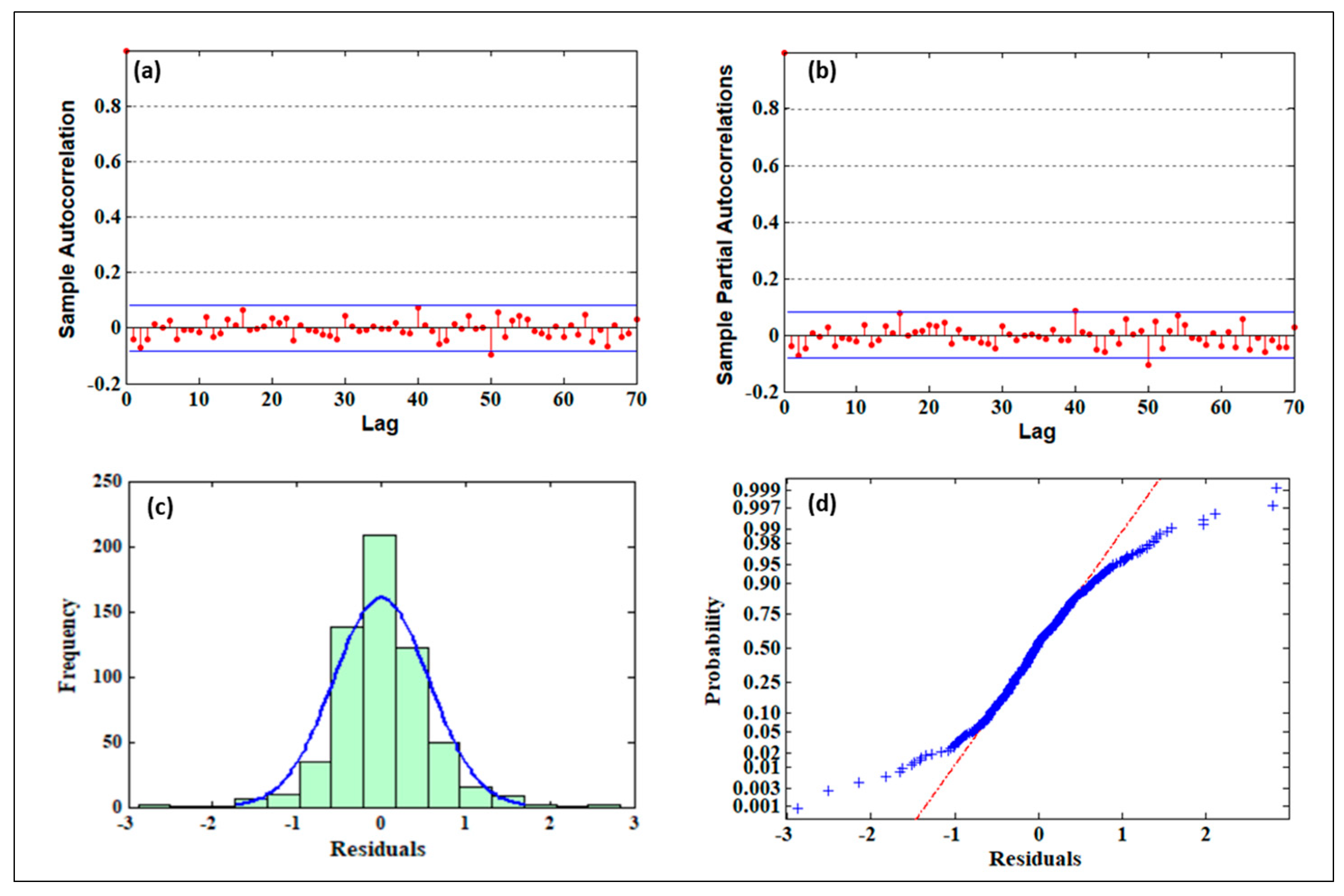
After finishing the parameter estimation, additional procedures confirmed that the generated residuals were independent, had normal probability distributions, and were of constant variance (conditional heteroscedasticity). The uncorrelatedness of residuals was investigated using a correlogram (Figure 6a,b) and the Ljung–Box Q-test for residual auto-correlation. Figure 5 shows that most of the residual ACF and PACF values were inside the confidence zone, indicating that there was insignificant correlation between them. Furthermore, at a significance level of 0.01, the Ljung–Box Q-test confirmed that the residuals were not auto-correlated. Figure 6c,d depict the histogram and normal probability plots of the SPI_3 residuals, respectively. According to the histogram, the residuals were generally centered on zero and almost normally distributed. Furthermore, they existed on a diagonal line that reflected their normality, as shown by the normal probability plot. The Engle test for residual heteroscedasticity failed to reject the null hypothesis of no conditional heteroscedasticity, confirming that the model was well-fitted. The above tests confirmed that the investigated model was appropriate for the associated SPI time-series.

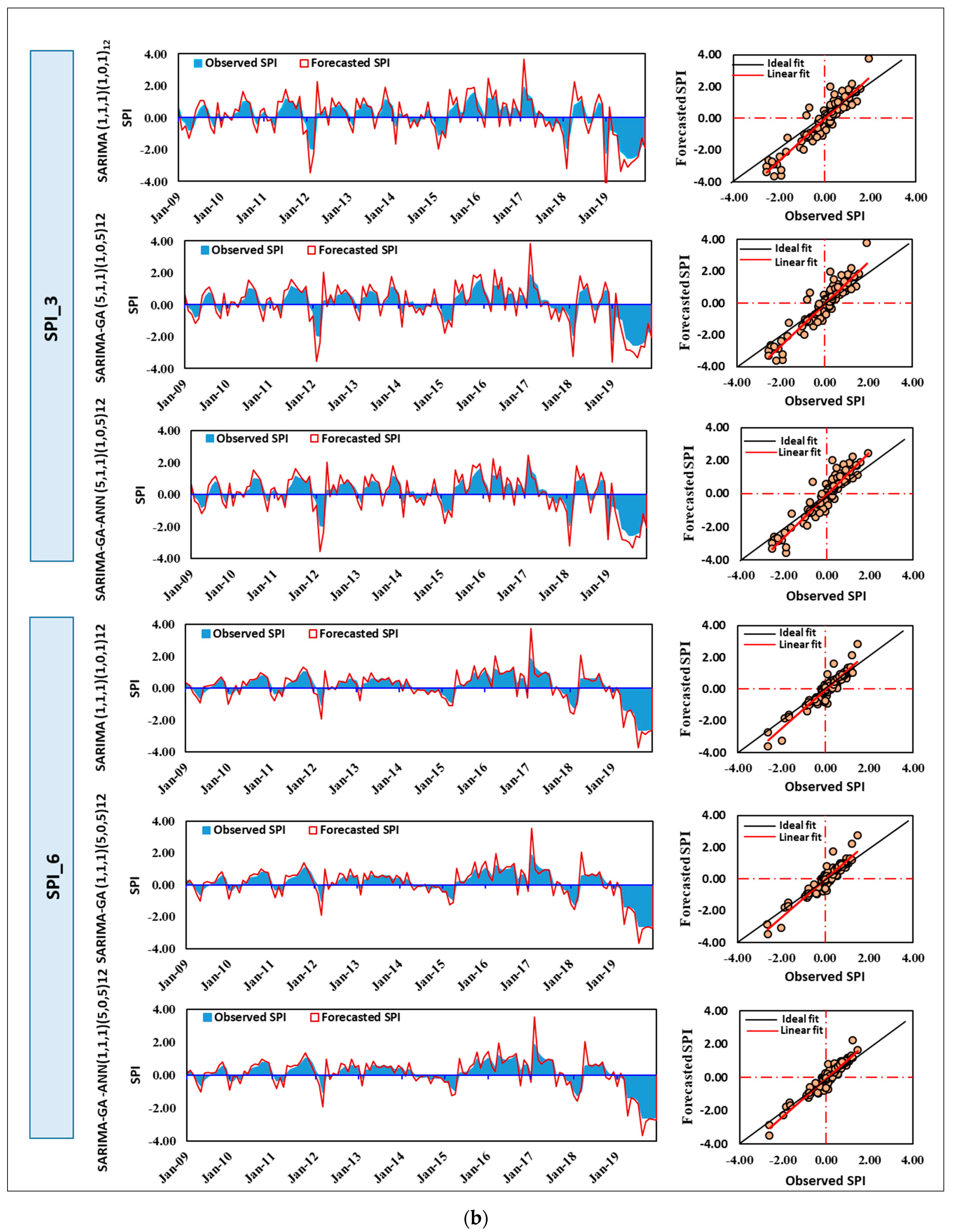
All of the previous steps were also applied to the drought indices SPI_6, SPI_9, SPI_12, and SPI_24, the results of which are presented in Table 3. After selecting the best model using GA-based ARIMA, drought forecasting was performed for the period 2009–2019, and the results were compared with historical records. Figure 7 presents a comparative analysis of historical and forecasted SPI in the testing period, while

Table 4. Performance criteria of the developed models for SARIMA and SARIMA–GA models.

	SPI Time Series	Model	R2	RMSE	MAD	E
Training	SPI_3	SARIMA (1,1,1)(1,0,1)12	0.821	0.559	0.457	0.624
		SARIMA–GA (5,1,1)(1,0,5)12	0.886	0.521	0.417	0.747
		SARIMA–GA–ANN (5,1,1)(1,0,5)12	0.932	0.483	0.398	0.752
	SPI_6	SARIMA (1,1,1)(1,0,1)12	0.868	0.315	0.274	0.827
		SARIMA–GA (1,1,1)(5,0,5)12	0.928	0.304	0.224	0.884
		SARIMA–GA–ANN (1,1,1)(5,0,5)12	0.949	0.282	0.193	0.914
	SPI_9	SARIMA (1,1,1)(1,0,1)12	0.872	0.239	0.243	0.859
		SARIMA–GA (5,1,5)(1,0,1)12	0.932	0.226	0.183	0.926
		SARIMA–GA–ANN (5,1,5)(1,0,1)12	0.956	0.177	0.167	0.954
	SPI_12	SARIMA (1,1,1)(1,0,1)12	0.886	0.175	0.204	0.877
		SARIMA–GA (1,1,1)(1,0,5)12	0.936	0.164	0.134	0.952
		SARIMA–GA–ANN (1,1,1)(1,0,5)12	0.963	0.145	0.112	0.961
	SPI_24	SARIMA (1,1,1)(1,0,1)12	0.893	0.171	0.181	0.894
		SARIMA–GA (1,1,1)(1,0,5)12	0.948	0.099	0.101	0.976
		SARIMA–GA–ANN (1,1,1)(1,0,5)12	0.976	0.051	0.086	0.983
Testing	SPI_3	SARIMA (1,1,1)(1,0,1)12	0.822	0.669	0.478	0.502
		SARIMA–GA (5,1,1)(1,0,5)12	0.873	0.561	0.438	0.642
		SARIMA–GA–ANN (5,1,1)(1,0,5)12	0.911	0.502	0.403	0.733
	SPI_6	SARIMA (1,1,1)(1,0,1)12	0.853	0.443	0.298	0.719
		SARIMA–GA (1,1,1)(5,0,5)12	0.914	0.395	0.248	0.779
		SARIMA–GA–ANN (1,1,1)(5,0,5)12	0.925	0.301	0.205	0.779
	SPI_9	SARIMA (1,1,1)(1,0,1)12	0.848	0.395	0.264	0.710
		SARIMA–GA (5,1,5)(1,0,1)12	0.908	0.327	0.204	0.788
		SARIMA–GA–ANN (5,1,5)(1,0,1)12	0.913	0.241	0.176	0.864
	SPI_12	SARIMA–GA (1,1,1)(1,0,1)12	0.867	0.276	0.193	0.804
		SARIMA–GA (1,1,1)(1,0,5)12	0.921	0.235	0.123	0.876
		SARIMA–GA–ANN (1,1,1)(1,0,5)12	0.933	0.167	0.095	0.921
	SPI_24	SARIMA (1,1,1)(1,0,1)12	0.862	0.22	0.161	0.819
		SARIMA–GA (1,1,1)(1,0,5)12	0.926	0.182	0.081	0.910
		SARIMA–GA–ANN (1,1,1)(1,0,5)12	0.945	0.157	0.061	0.957

summarizes the evaluation results of ARIMA and ARIMA–GA in forecasting the SPI at Abha Station. The classical ARIMA model had obviously lower accuracy than the evolutionary ARIMA–GA models in the training and testing phases. In the case of SPI_3, for the training phase, the performance measures of the SARIMA model were R² = 0.821, RMSE = 0.529, MAD = 0.4577, and E = 0.624. For the testing phase, R² = 0.822, RMSE = 0.669, MAD = 0.478, and E = 0.502. Considering the performance indices, the SARIMAA–GA model had better accuracy than the SARIMA model, where the training performance measures were R² = 0.876, RMSE = 0.520, MAD = 0.417, and E = 0.747. The values for the testing period were R² = 0.873, RMSE = 0.556, MAD = 0.438, and E = 0.642.

3.3. Hybrid ARIMA–GA–ANN Model

The ANN model was fitted to the residuals obtained after fitting the ARIMA–GA model. The input nodes represent the previously lagged residuals of the observations, while the output nodes are the forecasted values for the future. On the basis of the back-propagation training approach, a three-layer ANN model was constructed, with hidden nodes using the widely used sigmoid activation function and the output layer using the linear function. Since the number of nodes within the hidden layer of the constructed ANN model impacts significantly the performance of the model, the optimum number of neurons in this layer was achieved through a trial-and-error technique by varying the number of neurons. The training process would be completed when the RMSE of all tested datasets were reduced to a minimum. The best performance during the testing period was obtained with nine nodes in the hidden layer. By combining the output of the ANN and the output of the selected linear ARIMA–GA model, the hybrid ARIMA–GA–ANN models was obtained, and the results were compared with historical records. In the case of SPI_3, the performance indices showed that the SARIMA–GA–ANN model had better accuracy than the SARIMA–GA model, where the training performance measures were R² = 0.932, RMSE = 0.483, MAD = 0.398, and E = 0.752. The values for the testing period were R² = 0.911, RMSE = 0.502, MAD = 0.403, and E = 0.733.

3.4. HMM and Hybrid HMM–GA Models

The SPI data used in the ARIMA model were taken as the training and testing data for the HMM. The initial transition probability matrix, initial emission probability matrix, and steady-state probability were determined using a classical HMM. The trained HMM was then passed as an initial matrix for optimizing the HMM parameters during the simulation process in the GA. The pre-defined parameters were taken as an initial population as input to the GA during the simulation. Optimal selection of the HMM parameters was achieved using the GA to optimize the RMSE with a population size of 250, a crossover rate of 0.8, a mutation rate of 0.01, and 200 iterations. The average number of states was around 7, which seemed to support the calculated categories of drought in the study area. In this phase, the number of states remained roughly constant, while the fitness value continued to rise, indicating that the model found a local optimum and was still evolving. Once the global best-performing HMM model was selected through this process, the forecasted values of the selected model were estimated, and the forecasted and measured values were compared.

Figure 8 illustrates the measured and forecasted SPI and scatterplot for the HMM and HMM–GA models during the testing phase. The results indicated that the HMM–GA model achieved further improvements by reducing scatter in the forecast inflow. The performance criteria showed that the HMM–GA model performed better than the HMM. In the case of the training phase for SPI_3, the performance measures for the HMM (

Table 5. Performance criteria of the developed HMM and HMM–GA models.

	SPI	Model	R2	RMSE	MAD	E
Training	SPI_3	HMM	0.892	0.414	0.338	0.688
		HMM–GA	0.926	0.385	0.309	0.823
	SPI_6	HMM	0.915	0.262	0.203	0.885
		HMM–GA	0.938	0.233	0.166	0.946
	SPI_9	HMM	0.923	0.212	0.180	0.919
		HMM–GA	0.951	0.177	0.135	0.991
	SPI_12	HMM	0.935	0.173	0.151	0.938
		HMM–GA	0.953	0.125	0.099	0.978
	SPI_24	HMM	0.943	0.127	0.134	0.957
		HMM–GA	0.975	0.073	0.075	0.984
Testing	SPI_3	HMM	0.863	0.495	0.354	0.637
		HMM–GA	0.917	0.411	0.324	0.787
	SPI_6	HMM	0.896	0.328	0.221	0.769
		HMM–GA	0.928	0.265	0.184	0.834
	SPI_9	HMM	0.915	0.292	0.195	0.760
		HMM–GA	0.937	0.238	0.151	0.843
	SPI_12	HMM	0.93	0.204	0.143	0.860
		HMM–GA	0.966	0.142	0.091	0.937
	SPI_24	HMM	0.945	0.163	0.119	0.876
		HMM–GA	0.972	0.098	0.060	0.974

) were R² = 0.892, RMSE = 0.414, MAD = 0.338, and E = 0.668. For the testing phase, they were R² = 0.863, RMSE = 0.495, MAD = 0.354, and E = 0.637. In view of the performance indices, the HMM–GA model had better accuracy than the HMM model as illustrated in Table 5, with performance measures of R² = 0.920, RMSE = 0.385, MAD = 0.309, and E = 0.823 during training. For the testing period, these values were R² = 0.917, RMSE = 0.495, MAD = 0.354, and E = 0.787.

4. Discussion and Comparison of the Forecasting Models

We compared the hydrological performance of five drought forecasting models: ARIMA, ARIMA–GA, ARIMA–GA–ANN, HMM, and HMM–GA. The comprehensive analysis, performed in the evaluation of the five models (Table 4 and Table 5), revealed variation in their performance. The statistical indices used to evaluate the models (R², RMSE, MAD, and E) revealed that both ARIMA–GA–ANN and HMM–GA outperformed the other three models with very closely results and produced the highest R², the minimum RMSE, and maximum E. The ARIMA and HMM models exhibited a slight decrease in performance from the training phase to the testing phase; however, the drop in performance measures produced by HMM was comparatively high.

According to the statistical indices in Table 4 and Table 5, the models with GA performed considerably better than those without, and the GA improved the forecasting accuracy in both the training and testing phases. Consequently, the RMSE values of ARIMA–GA were reduced by an average of 10.06% and 9.36%, respectively, in comparison with ARIMA, in the training and testing phases. In addition, the R² values of ARIMA–GA increased by 6.68% and 6.64%, respectively, compared to ARIMA, in training and testing. Furthermore, modeling of the residuals of the ARIMA-GA model using ANN enhanced the forecasting accuracy of the hybrid ARIMA–GA with an average reduction of 20% in RMSE. The RMSE values of HMM–GA were reduced by 16.40% and 23.46%, respectively, compared with HMM, for training and testing. However, the R² values of HMM–GA model increased by an average of 2.93% and 3.71%, respectively, compared to HMM in training and testing.

These results confirmed the GA-induced improvement in both ARIMA and HMM due to the ability of the GA to find the parameters for the optimal solution of the two models. A paired Student’s t-test was performed to assess the statistical difference between the observed values and those forecasted by the four models. This test compared the means of the calculated and forecasted SPI, in order to determine whether the two vectors were statistically different. The h value for all tests was zero, and p values are presented in

Table 6. Results of the paired sample t-test applied to the observed and the forecasted values of the standardized precipitation index.

Model	Training				Testing
	SARIMA	SARIMA–GA	HMM	HMM–GA	SARIMA	SARIMA–GA	HMM	HMM–GA
	p
SPI_3	0.805	0.945	0.895	0.945	0.226	0.233	0.948	0.911
SPI_6	0.845	0.896	0.945	0.896	0.099	0.137	0.905	0.977
SPI_9	0.901	0.925	0.971	0.925	0.154	0.166	0.870	0.877
SPI_12	0.916	0.942	0.986	0.942	0.229	0.201	0.958	0.804
SPI_24	0.927	0.976	0.997	0.976	0.548	0.559	0.858	0.904

. All tests failed to reject the null hypothesis that the calculated SPI data and forecasted SPI data, for all time-scales, came from independent random samples with normal distributions and equal means. The ROC curves (Figure 9) represent the probability of detection (PoD) as a function of the false alarm rate (FAR) (see Supplementary Material). The ROC curves were significantly above the no-skill line for all drought categories and all SPI indices, confirming the ability of the proposed models.

Table 7. Area under the ROC curves for ARIMA–GA and HMM–GA models.

Model	SPI	SPI < –1	SPI < –1.5	SPI < –2
ARIMA–GA	SPI_3	0.635	0.657	0.685
	SPI_6	0.686	0.693	0.729
	SPI_9	0.712	0.736	0.778
HMM–GA	SPI 3	0.707	0.749	0.792
	SPI 6	0.793	0.809	0.857
	SPI 9	0.797	0.826	0.867

illustrates that the areas under the ROC curves, for the ARIMA–GA and HMM–GA models, were more than 0.5, confirming the ability of the proposed models to recognize events and non-events. Furthermore, Table 7 shows that HMM–GA was more skilled than ARIMA–GA and that the two models had the potential to be more skilled for extreme occurrences with higher SPI thresholds. An additional statistical evaluation was carried out to further investigate the model performance using the Taylor diagram (Figure 10), which describes the statistical characteristics of the models and their relative positions from the observed data set during the training and testing phases based on the RMSE and the triangle inequality comparison. Figure 10 confirms that both ARIMA–GA–ANN and HMM–GA models outperformed the other models, as it was the closest to the reference line (RMSE) and observed data sets in both training and testing phases for all SPI time-scales.

Further evaluation of the proposed models’ accuracy in drought forecasting at various lead time was performed.

Table 8. Performance measures for comparison of observed and forecasted data for SPI 3 and SPI6 for different lead times.

Model	SPI_3				SPI_6
	1-Month Lead		6-Month Lead		1-Month Lead		6-Month Lead
	R2	RMSE	R2	RMSE	R2	RMSE	R2	RMSE
SARIMA	0.822	0.669	0.503	0.823	0.853	0.443	0.522	0.786
SARIMA–GA	0.873	0.561	0.522	0.746	0.914	0.395	0.703	0.652
SARIMA–GA–ANN	0.911	0.502	0.634	0.721	0.925	0.301	0.761	0.563
HMM	0.863	0.495	0.613	0.663	0.896	0.328	0.563	0.584
HMM–GA	0.917	0.411	0.679	0.631	0.928	0.265	0.776	0.467

presents the forecasting results of SPI_3 and SPI_6 at 1-month and 6-month lead time. The forecasts of 6 months’ lead time, which included the outputs from forecasts of lead times of 1–5 months [15,36], confirmed that the forecast accuracy of all models decreased as the lead time increased.

The findings of our study supported the results of previous studies [40,41,59,60], which reported that employing a hybrid drought forecasting model enhanced the forecasting accuracy of the stand-alone model. For instance, Salisu and Shabriet [59] have proposed a hybrid Wavelet–ARIMA model and explored its ability to forecast drought using SPI data from January 1954 to December 2008. The comparison of their results revealed that the Wavelet was able to improve the forecasting accuracy of the hybrid model, as the mean square error decreased by an average value of 43%. Xu et al. [60] have proposed a hybrid ARIMA–support vector regression (SVR) model to forecast the SPI on multiple scales. Their results revealed that the proposed hybrid ARIMA–SVR model outperformed the classical ARIMA models. Mishra et al. [40] proposed integrating ARIMA with an ANN, and their results illustrated that the proposed hybrid model has the potential to provide much more reliable forecasting of the SPI series, compared with classical ANN and ARIMA models. Khan et al. [41] have combined the strengths of the wavelet transformation, ARIMA, and ANN in a new method for drought forecasting. Their results revealed that the ANN model achieved an average R-value of 0.423; however, the wavelet-based ANN model had an R-value of 0.415. Furthermore, they reported that wavelet–ANN–ARIMA achieved R values of 0.914 for the forecasted SPI. The aforementioned discussion and the findings of this study confirmed that our work added insight into the use of hybrid HMM–GA and ARIMA–GA to forecast meteorological drought.

5. Conclusions

In this study, we examined the potential of the ARIMA, ARIMA–GA, ARIMA–GA–ANN, HMM, and HMM–GA models for 1-month- and 6-months-ahead SPI forecasting. The models were evaluated using historical monthly rainfall data in the Bisha Valley, Saudi Arabia. Four statistical measures were used to assess their performance, and a Taylor diagram was presented to assess the correspondence between the calculated SPI and the output of each model. Generally, the results demonstrated that the ARIMA–GA–ANN and HMM–GA models provided more accurate forecasting compared to classical ARIMA and HMM. The performance of the models confirmed that the HMM–GA model was more capable than the ARIMA model of forecasting the SPI. Indeed, employing GA as an additional optimization algorithm in the HMM and ARIMA models improved the performance of both models significantly. Furthermore, considerable improvement of forecasting accuracy was achieved by combining the advantage of the linear ARIMA–GA model and non-linear ANN model. Based on the results and discussion, the main conclusion of this study is that integrating HMM and ARIMA with GA and ANN resulted in a highly valuable tool for meteorological drought forecasting.