
Modeling of Combined Lead Fast Reactor and Concentrating Solar Power Supercritical Carbon Dioxide Cycles to Demonstrate Feasibility, Efficiency Gains, and Cost Reductions


Abstract
:1. Introduction
- Monnerie et al. (2011): In search of an alternative to the typical fossil fuel-based process, reports on synthesizing hydrogen with complimentary solar-nuclear technologies being utilized as consistent heat sources for chemical decomposition of sulphuric acid to aid in simple, low-temperature electrolysis [17].
- Curtis J.D. (2015): Massachusetts Institute of Technology thesis reports cycle configuration, performance, and development of complimentary solar-nuclear systems with a focus on shale oil extraction and production from kerogen deposits [18].
- Wang et al. (2020): Implements a combined solar and nuclear plant discussing a sCO Brayton recompression cycle layout with an emphasis on a cycle design’s performance to varying solar irradiance and demonstration of feasibility [19].
2. Materials and Methods
2.1. Cycle Component Modeling
2.1.1. Turbines and Compressors
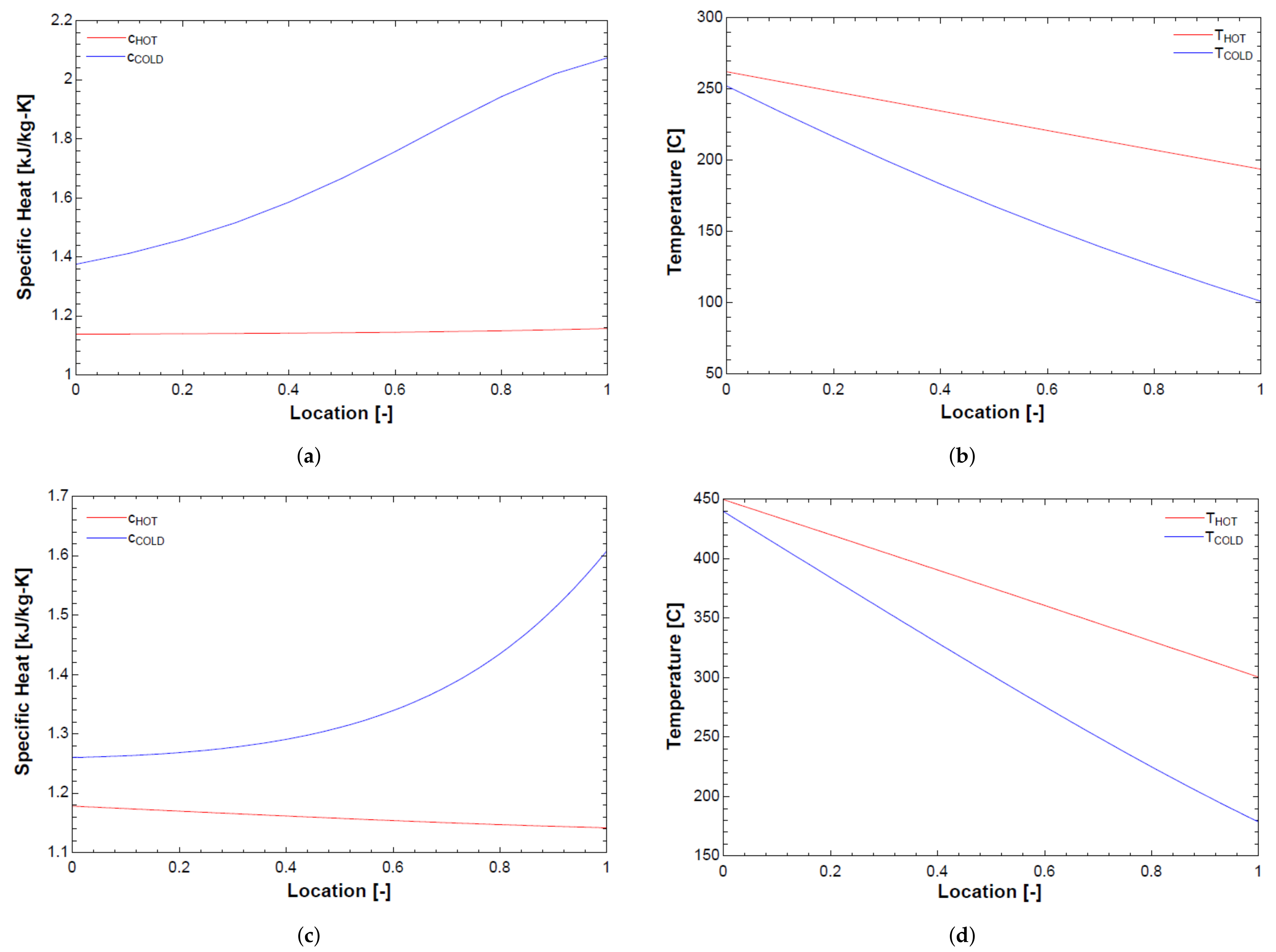
2.1.2. Black Box and Counter-Flow Heat Exchangers
2.1.3. Lead-Cooled Fast Reactor
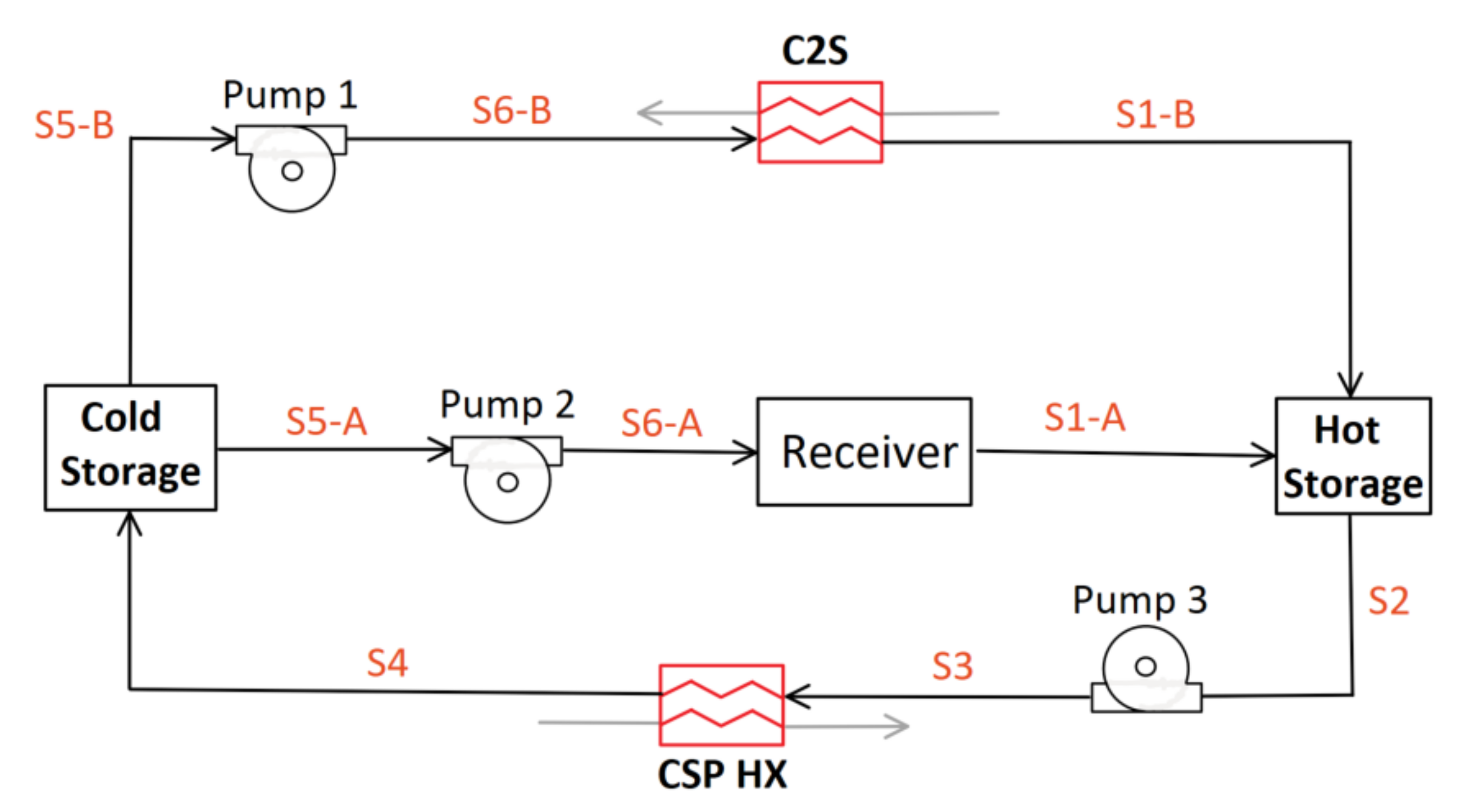
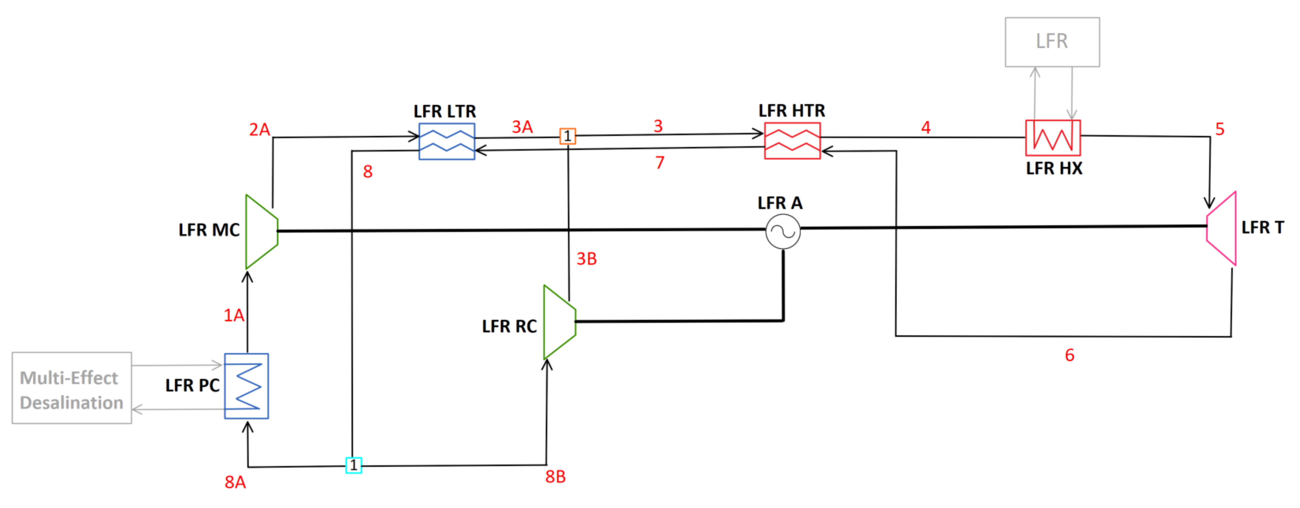
2.1.4. Concentrating Solar Power Cycle
2.2. Standardization of Cycle Modeling
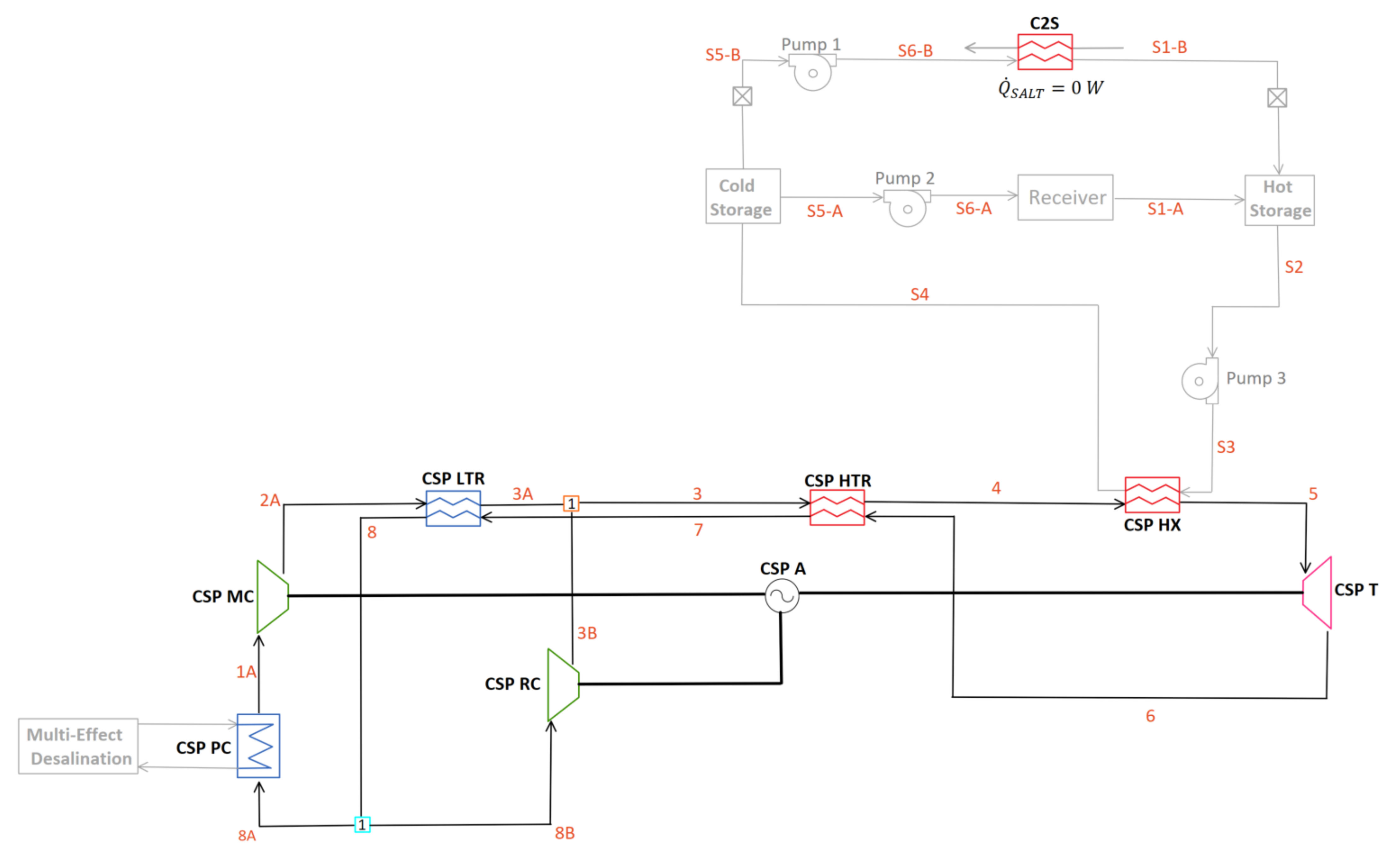
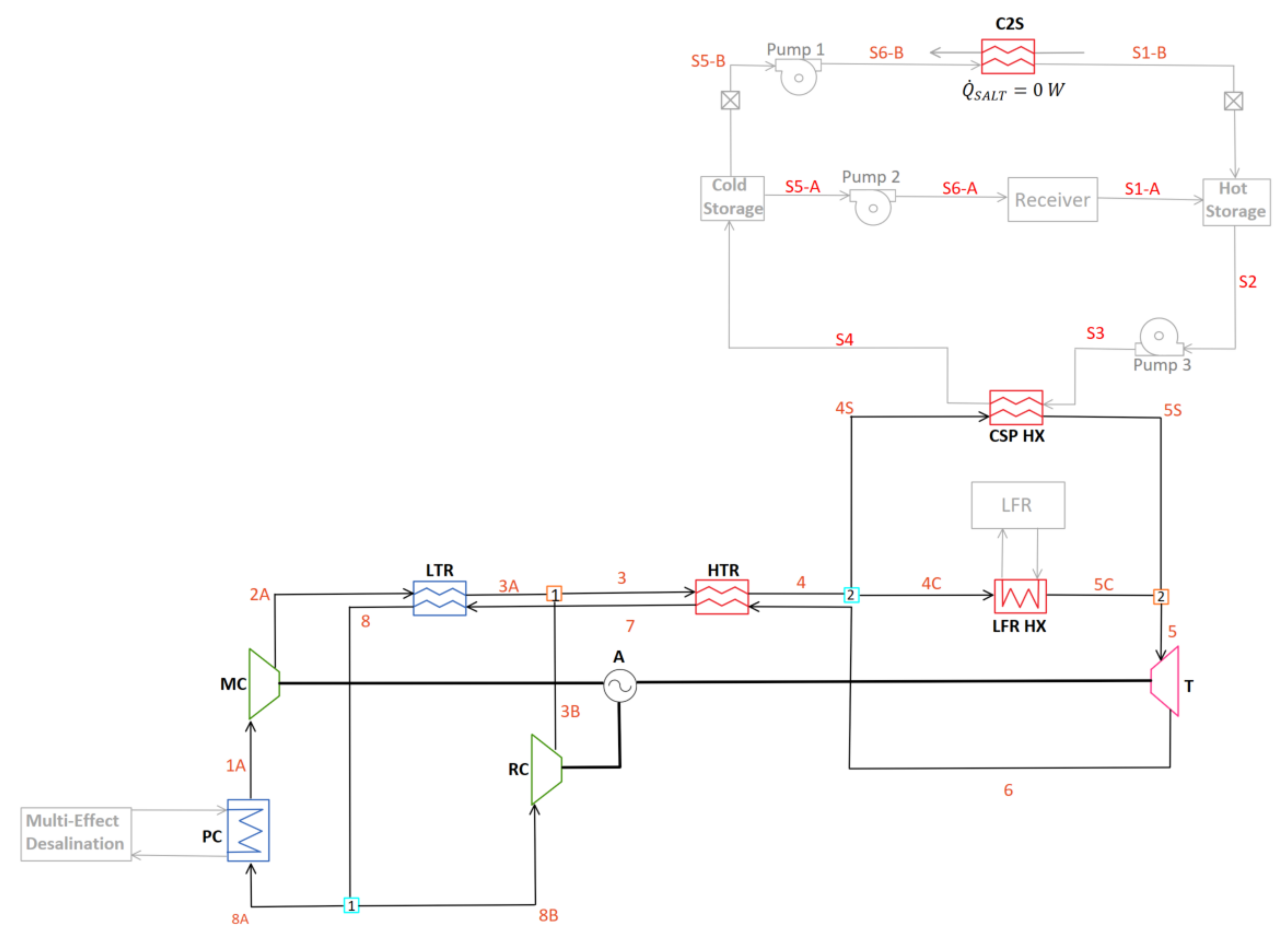
2.3. Non-Charging Cycle Configurations
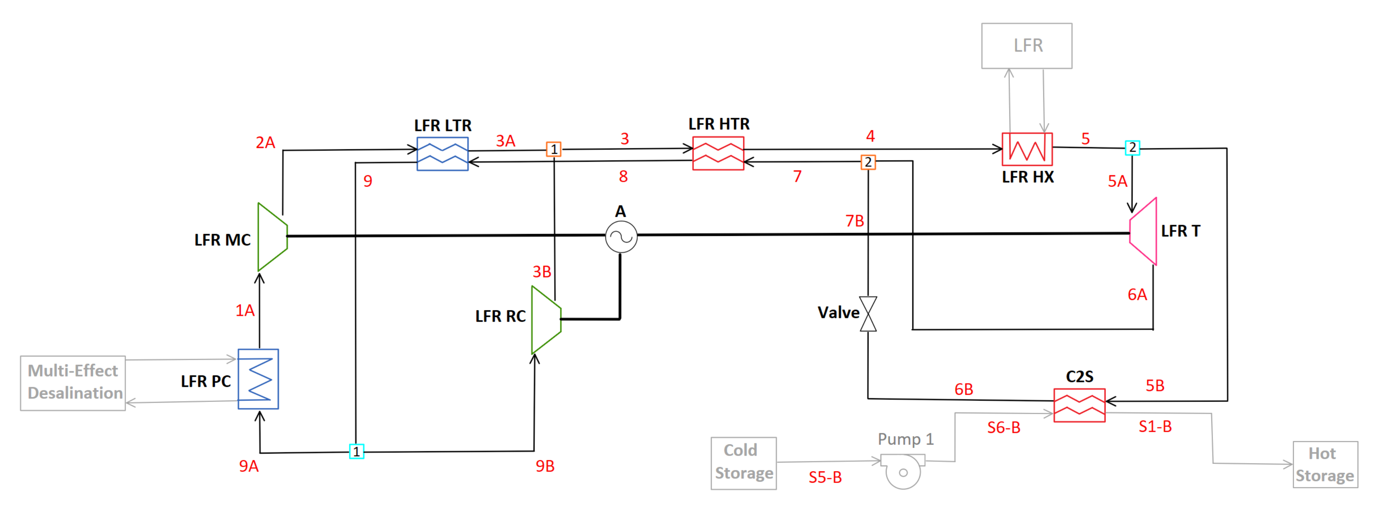
2.3.1. Two-Cycle Configuration: C-LFR-ON and C-CSP-ON
2.3.2. C-1HTR1T-ON
- C: Lowest cold TES temperature possible due to the sCO cold inlet constrained from the LFR to C and the addition of C approach temperature;
- C: Upper bound temperature on cold TES storage;
- C: Unconstrained LFR cold inlet temperature allows a lower cold TES of C to be achieved. This allows for a larger temperature drop across the CSP HX, increasing dispatchability.
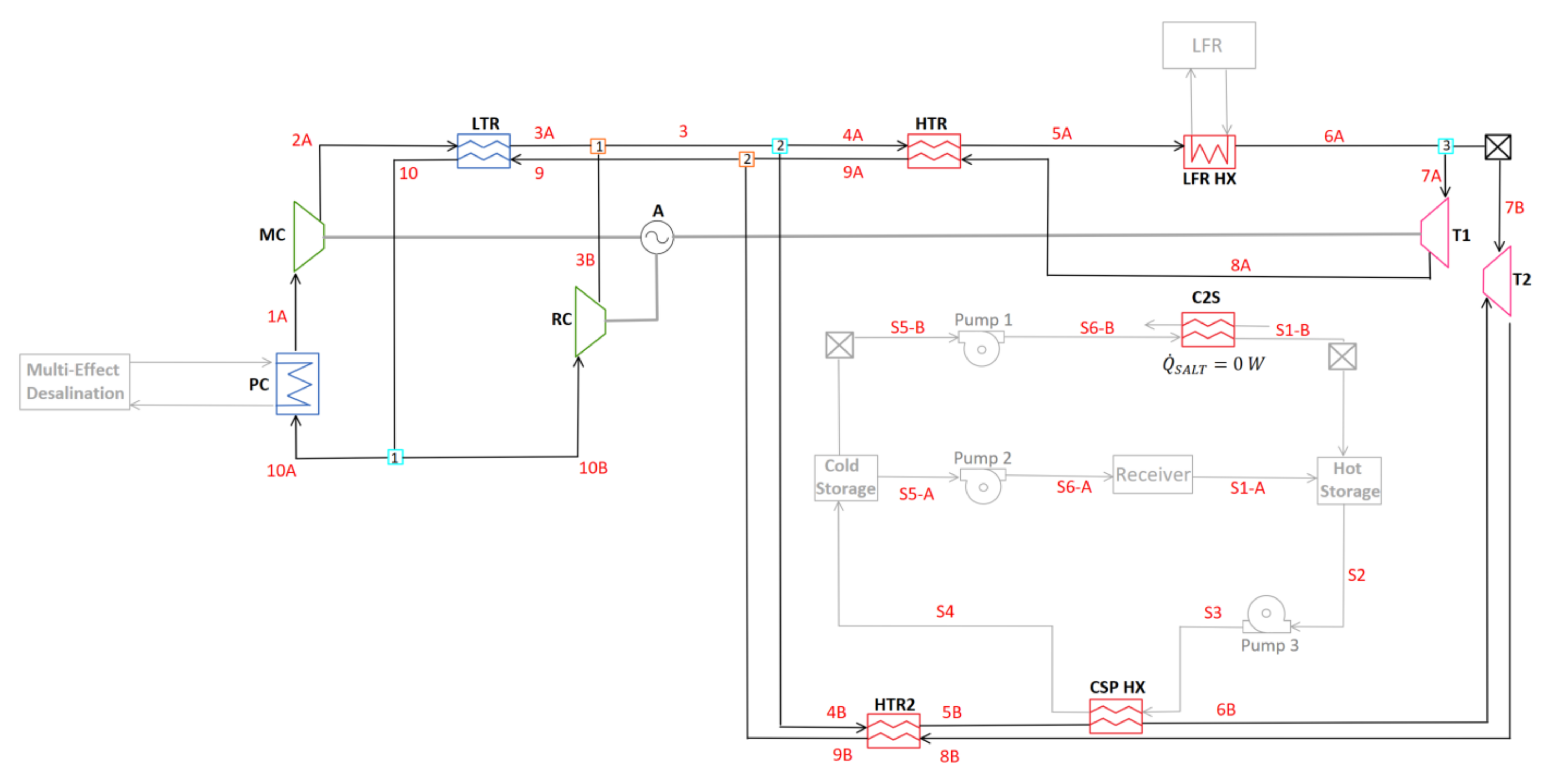
2.3.3. C-2HTR3T-ON
2.4. Thermal Energy Storage Charging Techniques
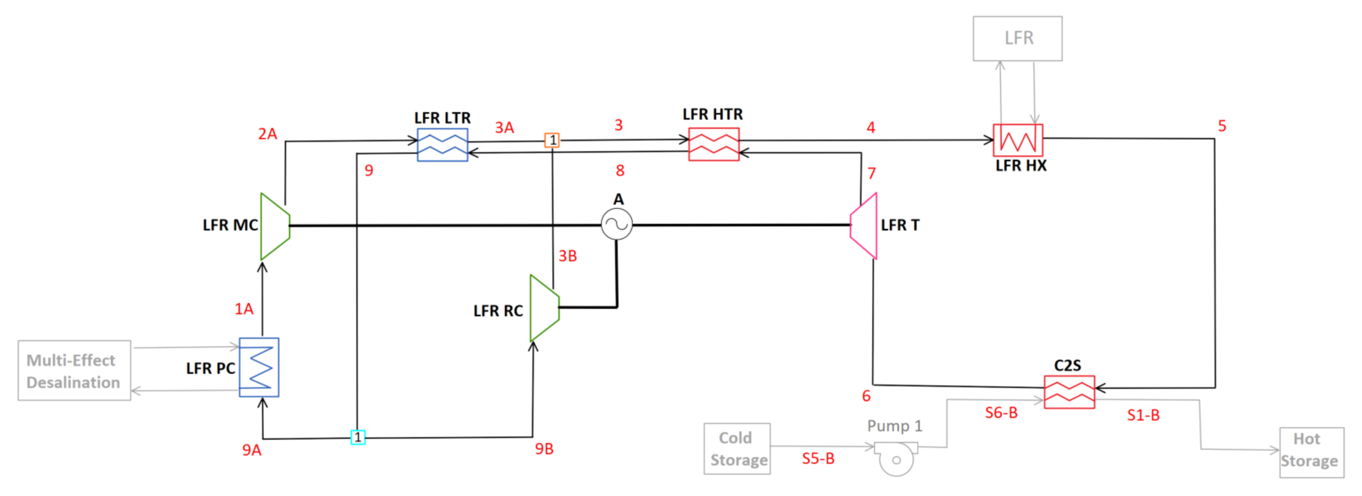
2.4.1. C-LFR-PRE
2.4.2. C-LFR-POST
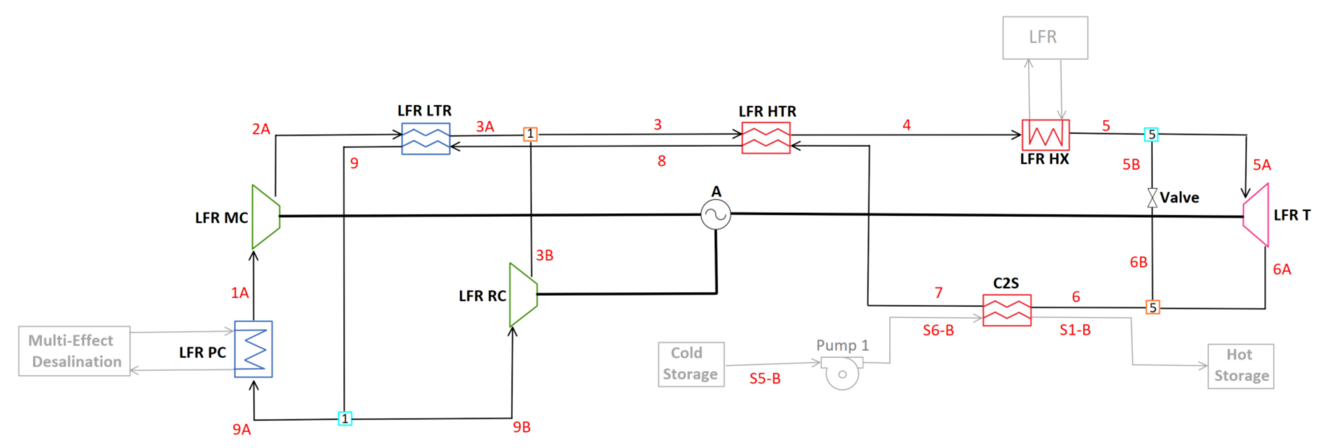
2.4.3. C-LFR-PAR
2.4.4. C-LFR-CIRC
3. Results and Discussion
3.1. Non-Charging Cycle Configurations
3.1.1. Two-Cycle Configuration: C-LFR-ON and C-CSP-ON
3.1.2. C-1HTR1T-ON
3.1.3. C-2HTR3T-ON
3.2. Thermal Energy Storage Charging Techniques
3.2.1. C-LFR-PRE
3.2.2. C-LFR-PAR
3.2.3. C-LFR-CIRC
4. Conclusions
- Two-cycle configuration C-LFR-ON and C-CSP-ON: Offers the highest cycle efficiency because of the freedom of the two cycles to operate independently when generating electrical power. The cycles individually are simple recompression but there is a lack of component synergies.
- C-1HTR1T-ON: Single-cycle configuration that is the least complex, and therefore cost efficient and compact, with heat additions from the CSP and LFR in parallel. With both CSP and LFR discharging, combined cycle efficiency is reduced by 0.8 percentage points compared to the two-cycle configuration.
- C-2HTR3T-ON: Single-cycle configuration that has dedicated turbines and HTRs for the LFR and CSP. This cycle makes a compromise between complexity with reduced cycle component redundancy, flexibility for dissimilar inlet temperatures on the CSP and LFR inlet, and median efficiency. The efficiency is only marginally higher than C-1HTR1T-ON, but heat storage efficiency when using the LFR to charge the salt is improved due to flexibility on setting the CSP and LFR inlet temperatures. As the additional turbines are likely present in practice anyway, this cycle is not anticipated to significantly increase cost and complexity over C-1HTR1T-ON. The relative merits of C-2HTR3T-ON and C-1HTR1T-ON are therefore similar. It is noted that for the unconstrained case C-2HTR3T achieves almost identical performance to the two-cycle configuration, with an efficiency of 46.1%, and hence the drop in performance relative to using separate cycles is attributable to the constraint on LFR inlet temperature being more limiting.
- C-LFR-POST: Charging technique with the turbine subsequent to C2S heat exchanger. Infeasible due to lower thermodynamic efficiency.
- C-LFR-PRE: Charging technique with the turbine prior to C2S heat exchanger with a valve that bypasses the turbine, demands a high outlet temperature for the LFR to be effective. Due to LFR outlet temperature limitations, this configuration has the next lowest heat storage efficiency.
- C-LFR-PAR: Charging technique that splits the flow directly after the LFR with the turbine and C2S heat exchanger in parallel. The heat storage efficiency is higher than C-LFR-PRE.
- C-LFR-CIRC: Flexible technique with a heat storage efficiency being highly dependent on cold TES temperature and LFR inlet temperature. Able to achieve heat storage efficiency to near 100% by eliminating losses associated with the turbines and compressors. For C-1HTR1T-ON, the heat storage efficiency is limit to 90% because the inlet temperatures to the LFR and CSP are constrained to be the same. The additional chiller and circulator components in the dedicated circulation loop increase complexity and cost.
Author Contributions
Funding
Data Availability Statement
Acknowledgments
Conflicts of Interest
Nomenclature
| Abbreviations | |
| A | Alternator |
| CSP | Concentrating solar power |
| C2S | sCO-to-Salt heat exchanger |
| EES | Engineering Equation Solver |
| HTR | High-temperature recuperator |
| HX | Heat exchanger |
| LFR | Lead-fast reactor |
| LTR | Low-temperature recuperator |
| MC | Main compressor |
| NREL | National Renewable Energy Laboratory |
| P | Pump |
| PC | Pre-cooler |
| RC | Re-compressor |
| sCO | Supercritical carbon dioxide |
| T | Turbine |
| TES | Thermal energy storage |
| Variables [Units] | |
| Capacitance ratio [-] | |
| Capacitance rate [MW/C] | |
| Temperature difference [C] | |
| Approach temperature of heat exchanger [C] | |
| Effectiveness of heat exchanger [-] | |
| Isentropic efficiency [-] | |
| h | Enthalpy [J/kg] |
| Mass flow rate [kg/s] | |
| Number of transfer units [-] | |
| P | Pressure [MPa] |
| Heat transfer rate [W] | |
| T | Temperature [C] |
| Conductivity of heat exchanger [MW/C] | |
| v | Volumetric flow rate [/kg] |
| Power [MW] | |
| y | Splitter fraction [-] |
References
- Turchi, C.S.; Ma, Z.; Neises, T.W.; Wagner, M.J. Thermodynamic study of advanced supercritical carbon dioxide power cycles for concentrating solar power systems. J. Sol. Energy Eng. 2013, 135, 041007. [Google Scholar] [CrossRef]
- Ahn, Y.H.; Bae, S.J.; Kim, M.S.; Cho, S.K.; Baik, S.J.; Lee, J.I.; Cha, J.E. Cycle layout studies of S-CO2 cycle for the next generation nuclear system application. In Proceedings of the The Korean Nuclear Society Autumn Meeting, Pyongchang, Korea, 29–31 October 2014. [Google Scholar]
- Wang, K.; Li, M.J.; Guo, J.Q.; Li, P.; Liu, Z.B. A systematic comparison of different S-CO2 Brayton cycle layouts based on multi-objective optimization for applications in solar power tower plants. Appl. Energy 2018, 212, 109–121. [Google Scholar] [CrossRef]
- Wright, S.A.; Pickard, P.S.; Fuller, R.; Radel, R.F.; Vernon, M.E. Supercritical CO2 Brayton Cycle Power Generation Development Program and Initial Test Results. In Proceedings of the ASME Power Conference, Albuquerque, NM, USA, 21–23 July 2009. [Google Scholar] [CrossRef]
- U.S. Department of Energy. Sunshot Vision Study. Available online: http://www1.eere.energy.gov/solar/sunshot/vision_study.html (accessed on 20 August 2021).
- Supercritical Carbon Dioxide Pilot Plant Test Facility. Available online: https://netl.doe.gov/project-information?p=FE0028979 (accessed on 30 August 2021).
- Brayton Energy. Available online: https://www.energy.gov/eere/solar/project-profile-brayton-energy (accessed on 30 August 2021).
- Iverson, B.D.; Conboy, T.M.; Pasch, J.J.; Kruizenga, A.M. Supercritical CO2 Brayton cycles for solar-thermal energy. Appl. Energy 2013, 111, 957–970. [Google Scholar] [CrossRef] [Green Version]
- Ho, C.K.; Carlson, M.; Garg, P.; Kumar, P. Cost and Performance Tradeoffs of Alternative Solar-Driven S-CO2 Brayton Cycle Configurations. In Proceedings of the ASME 2015 9th International Conference on Energy Sustainability collocated with the ASME 2015 Power Conference, the ASME 2015 13th International Conference on Fuel Cell Science, Engineering and Technology, and the ASME 2015 Nuclear Forum, San Diego, CA, USA, 28 June–2 July 2015; 2015. Available online: https://asmedigitalcollection.asme.org/ES/proceedings-pdf/ES2015/56840/V001T05A016/4448498/v001t05a016-es2015-49467.pdf (accessed on 30 August 2021).
- Neises, T. Steady-state off-design modeling of the supercritical carbon dioxide recompression cycle for concentrating solar power applications with two-tank sensible-heat storage. Sol. Energy 2020, 212, 19–33. [Google Scholar] [CrossRef]
- Dostal, V. A Supercritical Carbon Dioxide Cycle for Next Generation Nuclear Reactors. Ph.D. Thesis, Massachusetts Institute of Technology, Cambridge, MA, USA, 2004. [Google Scholar]
- Luo, D.; Huang, D. Thermodynamic and exergoeconomic investigation of various SCO2 Brayton cycles for next generation nuclear reactors. Energy Convers. Manag. 2020, 209, 112649. [Google Scholar] [CrossRef]
- Wright, S.A.; Conboy, T.M.; Rochau, G.E. Break-even Power Transients for two Simple Recuperated S-CO2 Brayton Cycle Test Configurations; Technical Report; Sandia National Lab. (SNL-NM): Albuquerque, NM, USA, 2011. [Google Scholar]
- Cha, J.E.; Bae, S.W.; Lee, J.; Cho, S.K.; Lee, J.I.; Park, J.H. Operation results of a closed supercritical CO2 simple Brayton cycle. In Proceedings of the 5th International Symposium-Supercritical CO2 Power Cycles, San Antonio, TX, USA, 28–31 March 2016; pp. 28–31. [Google Scholar]
- Held, T.J. Suipercritical CO2 Cycles for Gas Turbine Combined Cycle Power Plants. In Proceedings of the Power Gen International, Las Vegas, NV, USA, 8–10 December 2015. [Google Scholar]
- Fetvedt, J. Development of the sCO2 Allam Cycle. In Proceedings of the Supercritical CO2 Power Cycles Symposium, San Antonio, TX, USA, 29–31 March 2016. [Google Scholar]
- Monnerie, N.; Schmitz, M.; Roeb, M.; Quantius, D.; Graf, D.; Sattler, C.; De Lorenzo, D. Potential of hybridisation of the thermochemical hybrid-sulphur cycle for the production of hydrogen by using nuclear and solar energy in the same plant. Int. J. Nucl. Hydrog. Prod. Appl. 2011, 2, 178–201. [Google Scholar] [CrossRef]
- Curtis, D.J. Nuclear Renewable Oil Shale Hybrid Energy Systems: Configuration, Performance, and Development Pathways. Ph.D. Thesis, Massachusetts Institute of Technology, Cambridge, MA, USA, 2015. [Google Scholar]
- Wang, G.; Wang, C.; Chen, Z.; Hu, P. Design and performance evaluation of an innovative solar-nuclear complementarity power system using the S–CO2 Brayton cycle. Energy 2020, 197, 117282. [Google Scholar] [CrossRef]
- Turchi, C.S.; Vidal, J.; Bauer, M. Molten salt power towers operating at 600–650 C: Salt selection and cost benefits. Sol. Energy 2018, 164, 38–46. [Google Scholar] [CrossRef]
- Klein, S.; Nellis, G. Thermodynamics; Cambridge University Press: Cambridge, MA, USA, 2011. [Google Scholar] [CrossRef]
- Seidel, W. Model Development and Annual Simulation of the Supercritical Carbon Dioxide Brayton Cycle for Concentrating Solar Power Applications. Ph.D. Thesis, University of Wisconsin-Madison, Madison, WI, USA, 2010. [Google Scholar]
- Pacheco, J.E.; Ralph, M.E.; Chavez, J.M.; Dunkin, S.R.; Rush, E.E.; Ghanbari, C.M.; Matthews, M.W. Results of Molten Salt Panel and Component Experiments for Solar Central Receivers: Cold Fill, Freeze/thaw, Thermal Cycling and Shock, and Instrumentation Tests. 1995. Available online: https://www.osti.gov/servlets/purl/46671 (accessed on 30 August 2021).
- Span, R.; Wagner, W. A New Equation of State for Carbon Dioxide Covering the Fluid Region from the Triple-Point Temperature to 1100 K at Pressures up to 800 MPa. J. Phys. Chem. Ref. Data 1996, 25, 1509–1596. [Google Scholar] [CrossRef] [Green Version]
- Nellis, G.; Klein, S. Heat Transfer; Cambridge University Press: Cambridge, MA, USA, 2008. [Google Scholar] [CrossRef]
- Dyreby, J.J. Modeling the Supercritical Carbon Dioxide Brayton Cycle with Recompression. Ph.D. Thesis, University of Wisconsin-Madisom, Madison, WI, USA, 2014. [Google Scholar]
- Smith, C.; Cinotti, L. 6—Lead-cooled fast reactor. In Handbook of Generation IV Nuclear Reactors; Pioro, I.L., Ed.; Woodhead Publishing Series in Energy; Woodhead Publishing: Sawston, UK, 2016; pp. 119–155. [Google Scholar] [CrossRef]
- Alemberti, A.; Smirnov, V.; Smith, C.F.; Takahashi, M. Overview of lead-cooled fast reactor activities. Prog. Nucl. Energy 2014, 77, 300–307. [Google Scholar] [CrossRef]
- Mehos, M.; Turchi, C.; Vidal, J.; Wagner, M.; Ma, Z.; Ho, C.; Kolb, W.; Andraka, C.; Kruizenga, A. Concentrating Solar Power Gen3 Demonstration Roadmap; Technical Report; National Renewable Energy Lab. (NREL): Golden, CO, USA, 2017. [Google Scholar]
- Hamilton, W.T.; Husted, M.A.; Newman, A.M.; Braun, R.J.; Wagner, M.J. Dispatch optimization of concentrating solar power with utility-scale photovoltaics. Optim. Eng. 2020, 21, 335–369. [Google Scholar] [CrossRef]


| Parameter | Variable | Design Point Value |
|---|---|---|
| Efficiencies | ||
| Main Compressor | 0.91 (-) | |
| Re-Compressor | 0.89 (-) | |
| Turbine | 0.90 (-) | |
| Pumps 1–3 | 0.90 (-) | |
| Approach Temperatures | ||
| Low-Temperature Recuperator | 10 (C) | |
| High-Temperature Recuperator | 10 (C) | |
| Concentrating Solar Power Heat Exchanger | 10 (C) | |
| Pressures | ||
| Pressure Ratio | 3.27 (-) | |
| High Side Pressure | 28.8 (MPa) | |
| Heat into System | ||
| Lead-Cooled Fast Reactor Heat Transfer | 950 (MW) | |
| Concentrating Solar Power Heat Transfer | 750 (MW) | |
| Temperature | ||
| Main Compressor Inlet | 40 (C) | |
| Lead-Cooled Fast Reactor sCO High Temperature | ,,, | 595 (C) |
| Pumps | ||
| Pressure Rise across Pump | 3.726 (MPa) | |
| Pump Low Side Pressure | 3 (MPa) |
| Cycle Label | Description |
|---|---|
| Non-Charging | |
| C-LFR-ON | Two-cycle configuration with LFR as heat source. |
| C-CSP-ON | Two-cycle configuration with CSP as heat source. |
| C-1HTR1T-ON | CSP and LFR heat sources in parallel with one turbine. |
| C-2HTR3T-ON | CSP and LFR loops each with dedicated HTR and turbine. |
| Charging | |
| C-LFR-PRE | Turbine is prior to the C2S. |
| C-LFR-POST | Turbine is after the C2S. |
| C-LFR-PAR | Turbine is parallel to the C2S. |
| C-LFR-CIRC | Circulator bridges the LFR and C2S. |
| C-LFR-ON | C-CSP-ON | C-1HTR1T-ON | C-2HTR3T-ON | ||||||||
|---|---|---|---|---|---|---|---|---|---|---|---|
| Definition | Variable | U | C | N/A | N/A | U | C | C | U | C | C |
| Cycle Efficiency (%) | 47.08 | 45.28 | 45.58 | 45.93 | 44.9 | 44.22 | 44.22 | 46.10 | 44.34 | 44.35 | |
| LFR Inlet Temperature (C) | 415.1 | 400 | · | · | 380 | 400 | 400 | 415.2 | 400 | 400 | |
| Cold TES Temperature (C) | · | · | 390 | 440 | 390 | 410 | 440 | 390 | 390 | 440 | |
| Alternator Power (MW) | 447.3 | 430.2 | 339.1 | 340.6 | 763.9 | 752.3 | 752.6 | 783.7 | 753.7 | 754 | |
| PC Heat Transfer (MW) | 502.7 | 519.8 | 418.5 | 420.2 | 937.4 | 949.2 | 949.3 | 917.6 | 947.6 | 947.9 | |
| MC Power (MW) | 115 | 118.9 | 95.73 | 96.13 | 214.5 | 194.8 | 194.8 | 209.9 | 216.8 | 216.9 | |
| RC Power (MW) | 116.6 | 77.3 | 97.22 | 97.71 | 217.4 | 285.7 | 285.7 | 213.5 | 140.8 | 140.8 | |
| T1 Power (MW) | 678.9 | 626.4 | 532.1 | 534.5 | 1196 | 1233 | 1233 | 679.3 | 626.3 | 626.3 | |
| T2 Power (MW) | · | · | · | · | · | · | · | 527.8 | 485 | 485.4 | |
| MC Mass Flow Fraction (-) | 0.7 | 0.7844 | 0.6996 | 0.6994 | 0.7 | 0.6333 | 0.6333 | 0.6993 | 0.7846 | 0.7846 | |
| LFR Mass Flow Fraction (-) | · | · | · | · | 0.4485 | 0.4928 | 0.4929 | 0.5478 | 0.5486 | 0.5484 | |
| LTR UA Value (MW/C) | 54.68 | 22.84 | 45.4 | 45.53 | 102 | 91.63 | 91.64 | 134.4 | 41.56 | 41.57 | |
| LTR Capacitance Ratio (-) | 0.9867 | 0.8473 | 0.9858 | 0.9854 | 0.9867 | 0.9066 | 0.9066 | 0.9853 | 0.847 | 0.847 | |
| LTR Heat Transfer Rate (MW) | 656.8 | 366.5 | 548.3 | 551.4 | 549.2 | 614.9 | 615.1 | 1204 | 667.1 | 667.3 | |
| LTR Effectiveness (-) | 0.92 | 0.8742 | 0.9201 | 0.9202 | 0.92 | 0.9485 | 0.9485 | 0.9414 | 0.8741 | 0.8741 | |
| HTR UA Value (MW/C) | 48.29 | 42.71 | 34.58 | 34.72 | 78.22 | 82.3 | 82.34 | 48.32 | 42.69 | 42.69 | |
| HTR Capacitance Ratio (-) | 0.8657 | 0.8143 | 0.8593 | 0.8594 | 0.8595 | 0.8754 | 0.8755 | 0.8661 | 0.8142 | 0.8142 | |
| HTR Heat Transfer Rate (MW) | 998.1 | 1161 | 665.4 | 667.7 | 679.2 | 742.6 | 743 | 545.7 | 636.8 | 636.6 | |
| HTR Effectiveness (-) | 0.9544 | 0.9627 | 0.9436 | 0.9436 | 0.9445 | 0.9441 | 0.9441 | 0.9542 | 0.9627 | 0.9627 | |
| HTR2 UA Value (MW/C) | · | · | · | · | · | · | · | 34.29 | 31.61 | 31.63 | |
| HTR2 Capacitance Ratio (-) | · | · | · | · | · | · | · | 0.8594 | 0.8074 | 0.8074 | |
| HTR2 Heat Transfer Rate (MW) | · | · | · | · | · | · | · | 298.1 | 363.4 | 363.8 | |
| HTR2 Effectiveness (-) | · | · | · | · | · | · | · | 0.9436 | 0.9561 | 0.9561 | |
| CSPHX UA Value (MW/C) | · | · | 71.34 | 26.92 | 33.72 | 73.4 | 35.05 | 70.88 | 44.92 | 23.13 | |
| CSPHX Capacitance Ratio (-) | · | · | 0.9924 | 0.701 | 0.8104 | 0.9957 | 0.8034 | 0.9926 | 0.9138 | 0.6454 | |
| CSPHX Heat Transfer Rate (MW) | · | · | 757.6 | 760.8 | 751.3 | 751.5 | 751.9 | 751.3 | 751.3 | 751.9 | |
| CSPHX Effectiveness (-) | · | · | 0.945 | 0.945 | 0.945 | 0.9381 | 0.9374 | 0.9450 | 0.9493 | 0.9493 | |
| C-LFR-PRE | C-LFR-PAR | C-LFR-CIRC | |||||
|---|---|---|---|---|---|---|---|
| Definition | Variable | C | C | C | C | C | C |
| Cold TES Temperature (C) | 390 | 390 | 440 | 390 | 410 | 440 | |
| LFR Inlet Temperature (C) | 400 | 400 | 400 | 400 | 400 | 400 | |
| Heat Storage Efficiency (%) | 34.53 | 45.30 | 45.30 | 99.92 | 89.66 | 74.29 | |
| Alternator Power (MW) | 0 | 0 | 0 | · | · | · | |
| PC Heat Transfer (MW) | 622 | 519.6 | 519.6 | · | · | · | |
| MC Power (MW) | 142.3 | 118.9 | 118.9 | · | · | · | |
| RC Power (MW) | 21.89 | 77.28 | 77.28 | · | · | · | |
| Turbine Power (MW) | 164.2 | 196.2 | 196.2 | · | · | · | |
| Chiller Heat Transfer (MW) | · | · | · | 0.7245 | 98.25 | 244.2 | |
| MC Mass Flow Fraction (-) | 0.9389 | 0.7844 | 0.7844 | · | · | · | |
| C2S Mass Flow Fraction (-) | · | 0.6867 | 0.6867 | · | · | · | |
| Valve Mass Flow Fraction (-) | 0.7378 | · | · | · | · | · | |
| LTR UA Value (MW/C) | 6.99 | 22.83 | 22.83 | · | · | · | |
| LTR Capacitance Ratio (-) | 0.6754 | 0.8473 | 0.8743 | · | · | · | |
| LTR Heat Transfer Rate (MW) | 93.05 | 366.4 | 366.4 | · | · | · | |
| LTR Effectiveness (-) | 0.6384 | 0.8742 | 0.8742 | · | · | · | |
| HTR UA Value (MW/C) | 41.69 | 42.69 | 42.69 | · | · | · | |
| HTR Capacitance Ratio (-) | 0.7531 | 0.8143 | 0.8143 | · | · | · | |
| HTR Heat Transfer Rate (MW) | 1567 | 1160 | 1160 | · | · | · | |
| HTR Effectiveness (-) | 0.9695 | 0.9627 | 0.9627 | · | · | · | |
| C2S UA Value (MW/C) | 9.04 | 8.037 | 14.24 | 48.29 | 43.16 | 35.63 | |
| C2S Capacitance Ratio (-) | 0.4735 | 0.7556 | 0.9339 | 0.8755 | 0.8599 | 0.8294 | |
| C2S Heat Transfer Rate (MW) | 328 | 430.4 | 430.4 | 949.3 | 851.8 | 705.8 | |
| C2S Effectiveness (-) | 0.9368 | 0.8275 | 0.8307 | 0.9511 | 0.9459 | 0.9355 | |
| C2S Approach Temperature (C) | 10 | 35 | 26.27 | 10 | 10 | 10 | |
Publisher’s Note: MDPI stays neutral with regard to jurisdictional claims in published maps and institutional affiliations. |
© 2021 by the authors. Licensee MDPI, Basel, Switzerland. This article is an open access article distributed under the terms and conditions of the Creative Commons Attribution (CC BY) license (https://creativecommons.org/licenses/by/4.0/).
Share and Cite
White, B.T.; Wagner, M.J.; Neises, T.; Stansbury, C.; Lindley, B. Modeling of Combined Lead Fast Reactor and Concentrating Solar Power Supercritical Carbon Dioxide Cycles to Demonstrate Feasibility, Efficiency Gains, and Cost Reductions. Sustainability 2021, 13, 12428. https://doi.org/10.3390/su132212428
White BT, Wagner MJ, Neises T, Stansbury C, Lindley B. Modeling of Combined Lead Fast Reactor and Concentrating Solar Power Supercritical Carbon Dioxide Cycles to Demonstrate Feasibility, Efficiency Gains, and Cost Reductions. Sustainability. 2021; 13(22):12428. https://doi.org/10.3390/su132212428
Chicago/Turabian StyleWhite, Brian T., Michael J. Wagner, Ty Neises, Cory Stansbury, and Ben Lindley. 2021. "Modeling of Combined Lead Fast Reactor and Concentrating Solar Power Supercritical Carbon Dioxide Cycles to Demonstrate Feasibility, Efficiency Gains, and Cost Reductions" Sustainability 13, no. 22: 12428. https://doi.org/10.3390/su132212428
APA StyleWhite, B. T., Wagner, M. J., Neises, T., Stansbury, C., & Lindley, B. (2021). Modeling of Combined Lead Fast Reactor and Concentrating Solar Power Supercritical Carbon Dioxide Cycles to Demonstrate Feasibility, Efficiency Gains, and Cost Reductions. Sustainability, 13(22), 12428. https://doi.org/10.3390/su132212428