
Sensitivity of Riparian Buffer Designs to Climate Change—Nutrient and Sediment Loading to Streams: A Case Study in the Albemarle-Pamlico River Basins (USA) Using HAWQS

 ,
, 


Abstract
:1. Introduction
Objectives, Scope, and Novel Contribution
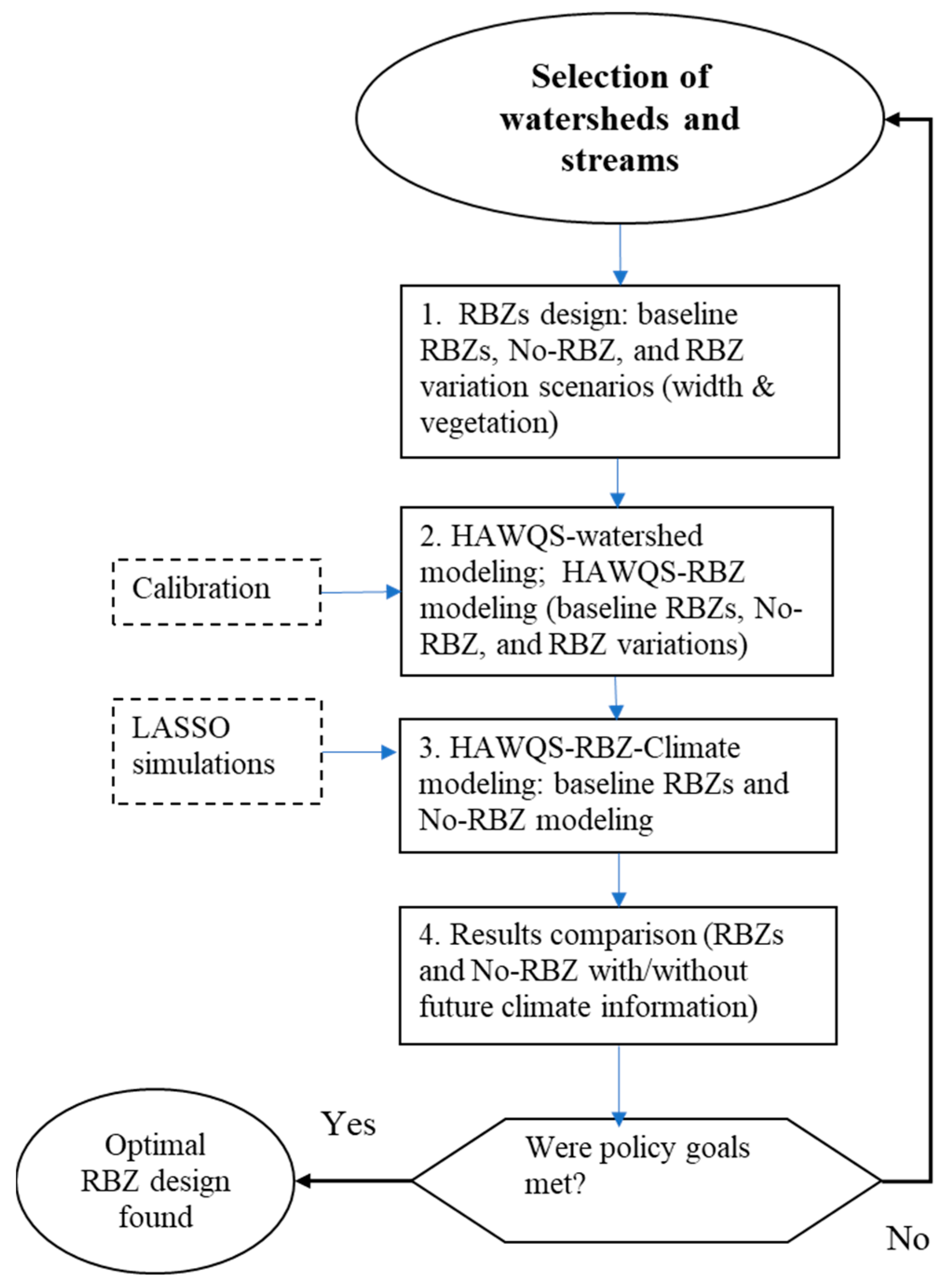
2. Material and Methods
2.1. Watershed Selection
2.2. RBZs Design
2.3. HAWQS Watershed Modeling and Calibration
2.4. HAWQS–RBZ Modeling
2.5. LASSO—Climate Modeling
- Definition of a study area: U.S. EPA Region and U.S. state level data were available (excluding Alaska, Hawaii, or the American Territories).
- Selection of a data source: bias corrected spatially downscaled (BCSD) and localized constructed analogs (LOCA) datasets were available. Each of these datasets represented downscaled information (i.e., translated into higher-resolution information that can be used as input to local or regional impact analyses, from the Coupled Model Intercomparison Project 5 (CMIP5) General Circulation Models (GCMs)) [54,56,57]. The LOCA dataset requires finer spatial resolution at 1/16° than that of BCSD at 1/8°; however, no one data source is better or more accurate than the other [54].
- Selection of an emission pathway: The moderate and rising emission scenarios known as the representative concentration pathways (RCP), RCP4.5 and RCP8.5, were available. RCP8.5 refers to the rising radiative forcing pathway (i.e., cumulative measure of human emissions of greenhouse gases (GHGs) from all sources expressed in Watts per square meter (W/m2)), leading to 8.5 W/m2 in 2100, and the RCP 4.5 refers to moderate stabilization without overshoot pathway to 4.5 W/m2 at stabilization after 2100 [56,58]. These two are the most frequently appearing RCPs in the literature.
- Selection of climate variables: climate variables (air temperature and precipitation) for five seasons (annual, winter, spring, summer, and fall) and three timeframes (2021–2050, 2041–2070, and 2070–2099) were available.
- Climate model selection strategies: Four climate model selection strategies were available within the LASSO tool that included LASSO, four corners, middle corners, and double median. Each strategy offers a subset of future climate projection models.
- Climate projection simulation and analysis: Given the numbers of data sources, RCPs, seasons, timeframes, and selection strategies, we used the “scenario discovery” [59] approach to obtain a manageable number of representative projections of precipitation (i.e., wettest and driest precipitation) and air temperature (i.e., hottest and coldest temperature) that served as input into the HAWQS modeling analysis. In this approach, we started a LASSO climate simulation for the State of NC by choosing a combination of LOCA, RCP8.5, the LASSO strategy for all the three timeframes, and five seasons (Table A4). The LASSO strategy was selected at first because it corresponded to the lowest risk tolerance, meaning it included the largest amount of information as compared to other strategies and was recommended by the LASSO tool [54]. We downloaded the spatial data, maps, and scatterplot graphics, compared future climate projection results to each other, and determined the extreme mean values of precipitation (i.e., wettest and driest precipitation) and air temperature (i.e., hottest and coldest temperature) for NC and VA.
2.6. HAWQS–RBZ Climate Modeling
3. Results
3.1. RBZ Designs and WQI Parameters
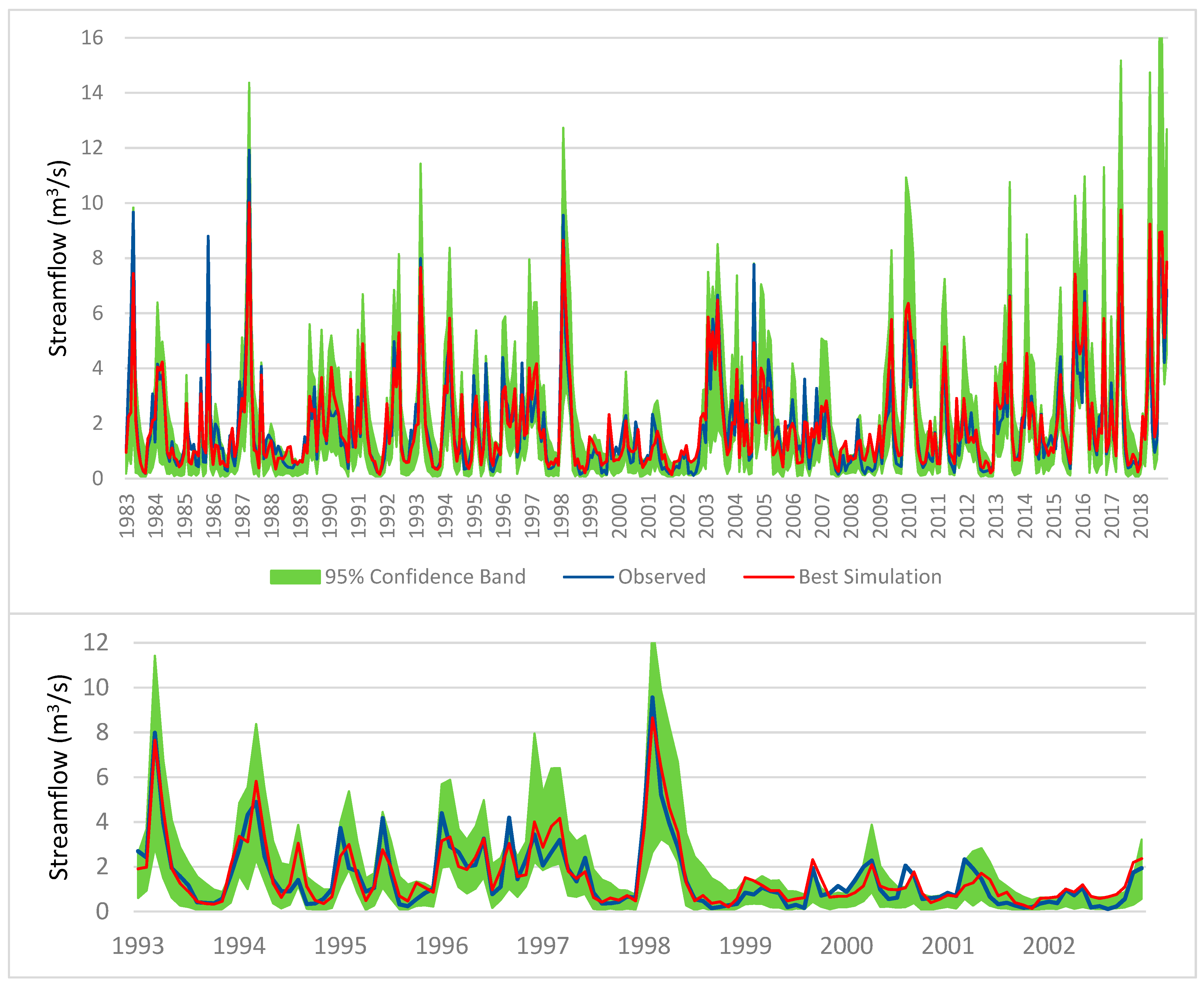
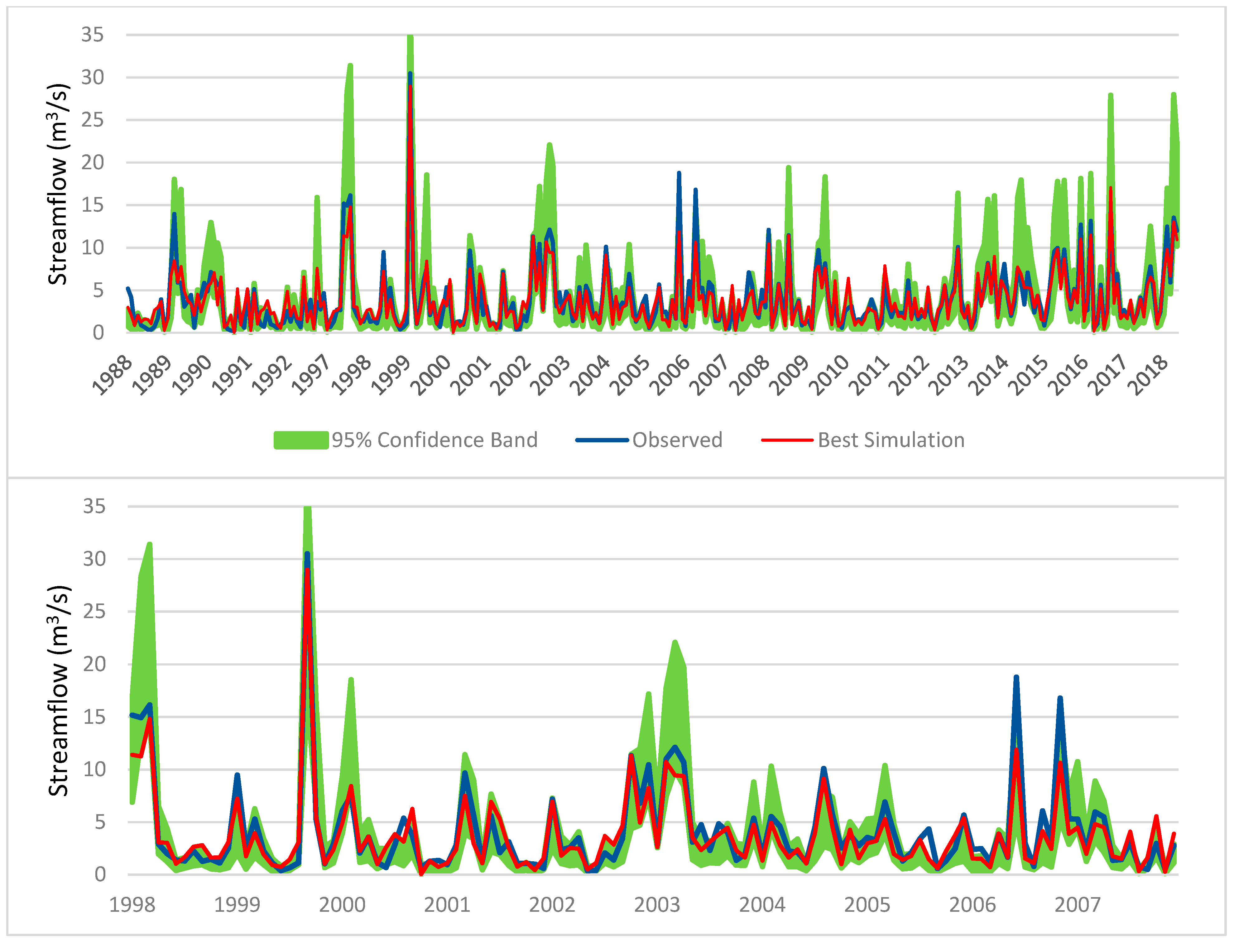
3.2. HAWQS Watershed Model Calibration
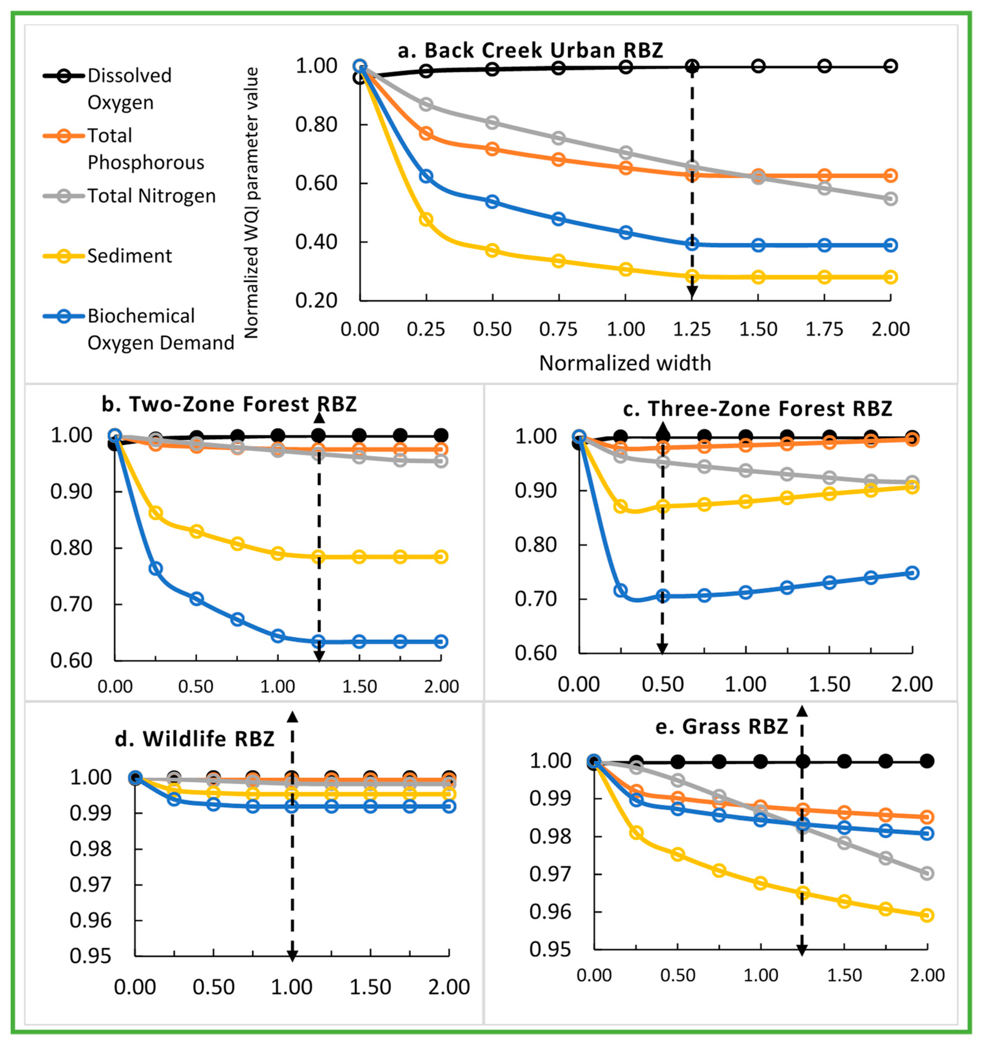
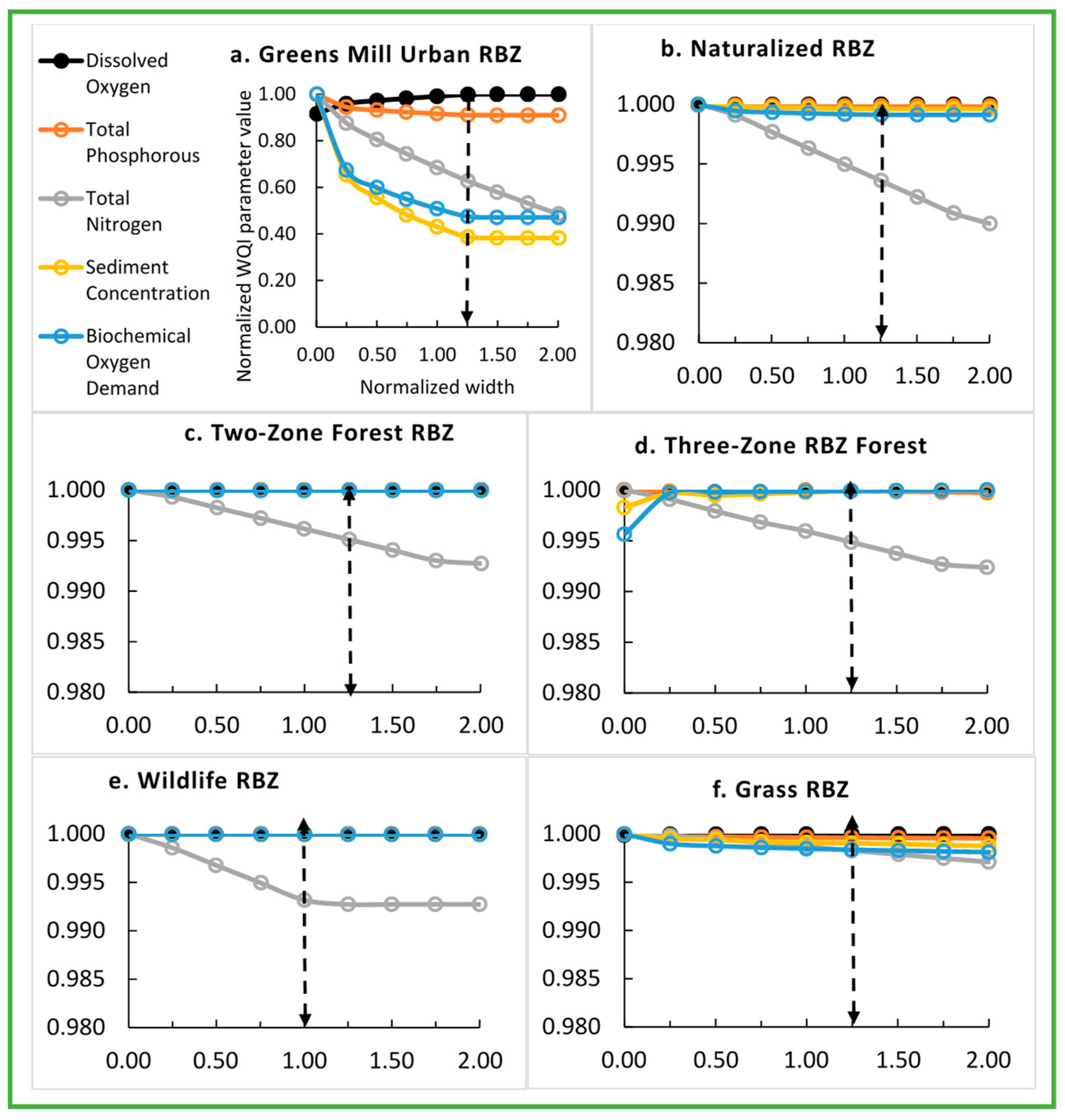
3.3. RBZ Sensitivity to WQI Parameters
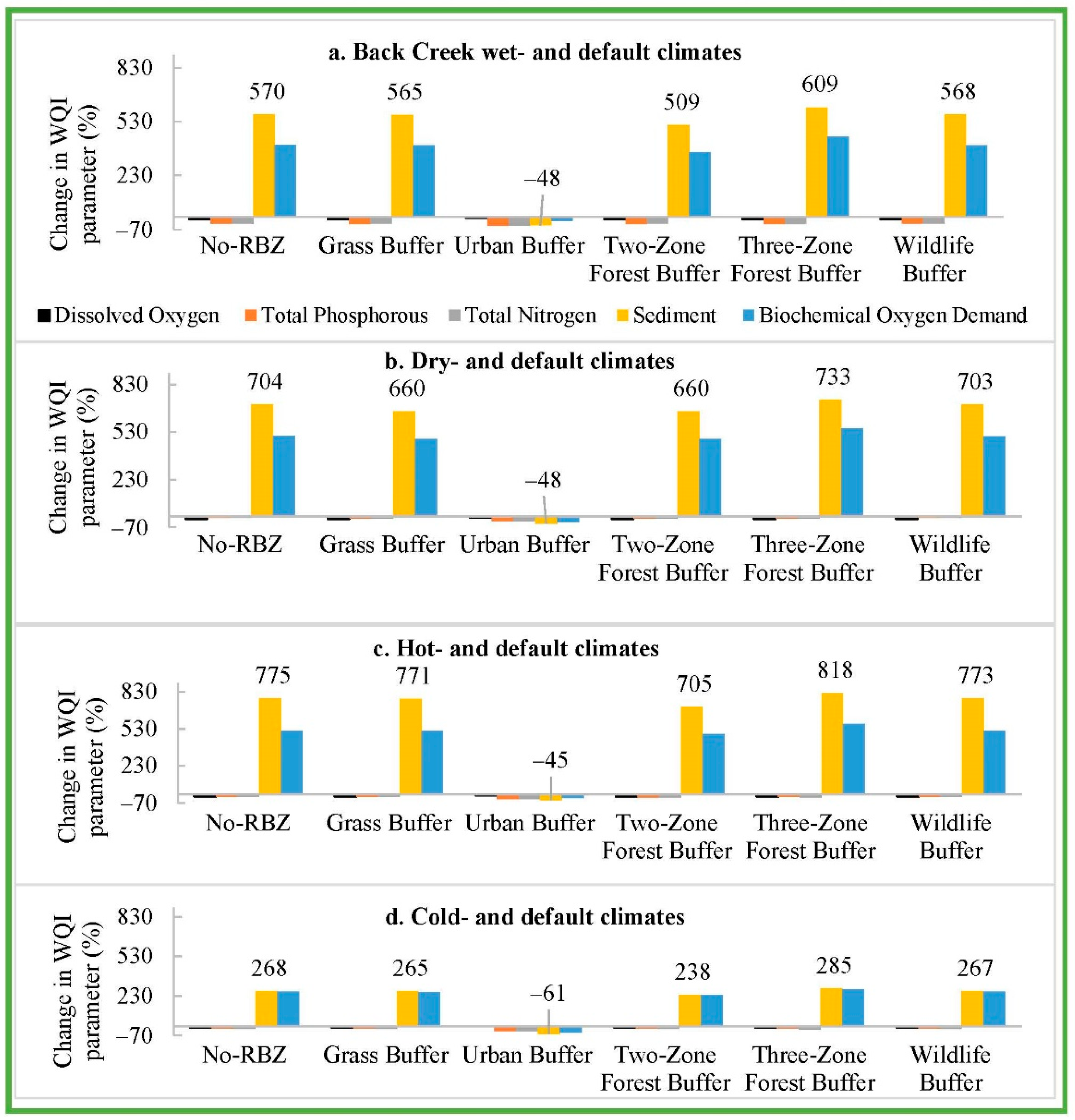
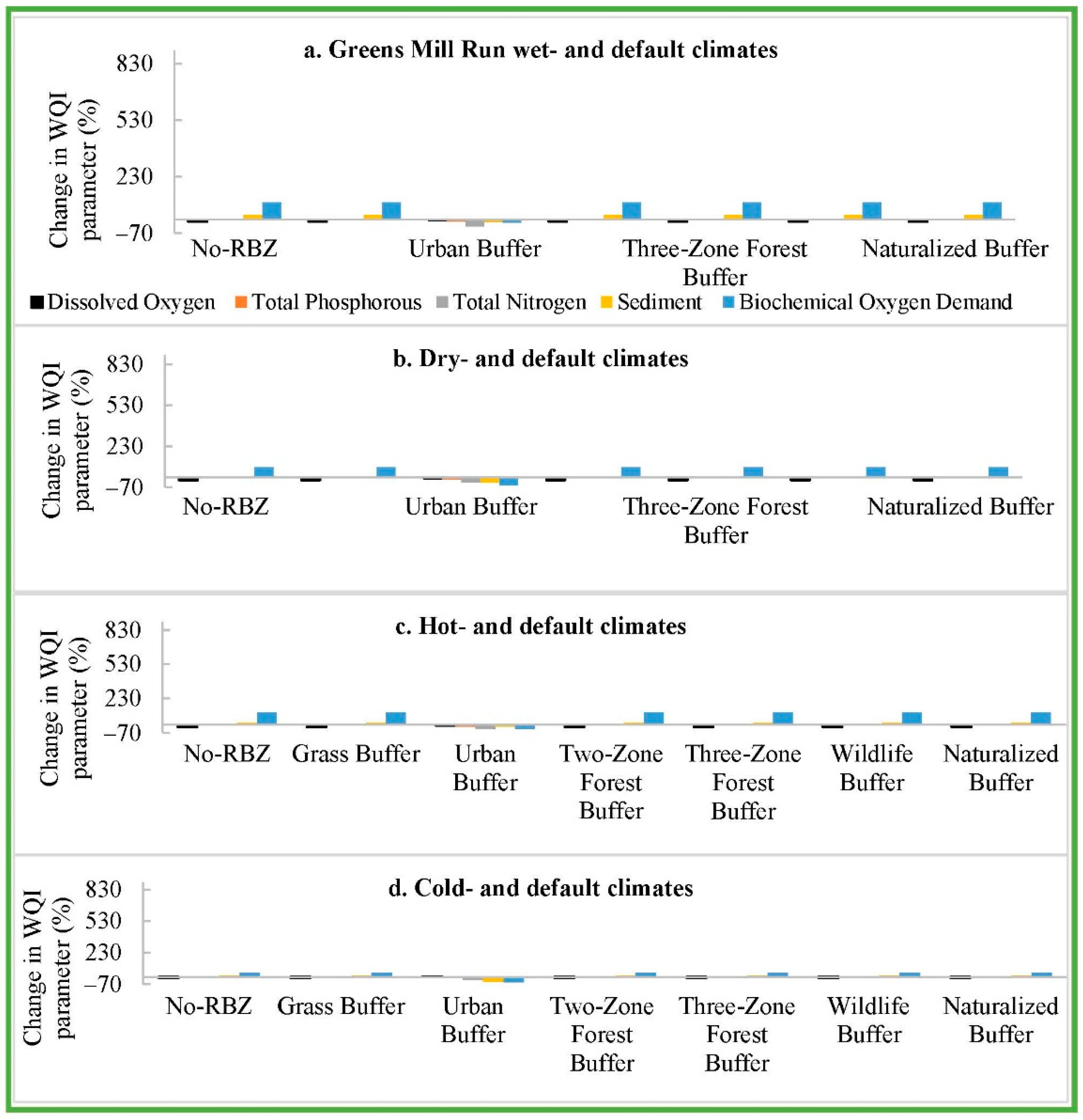
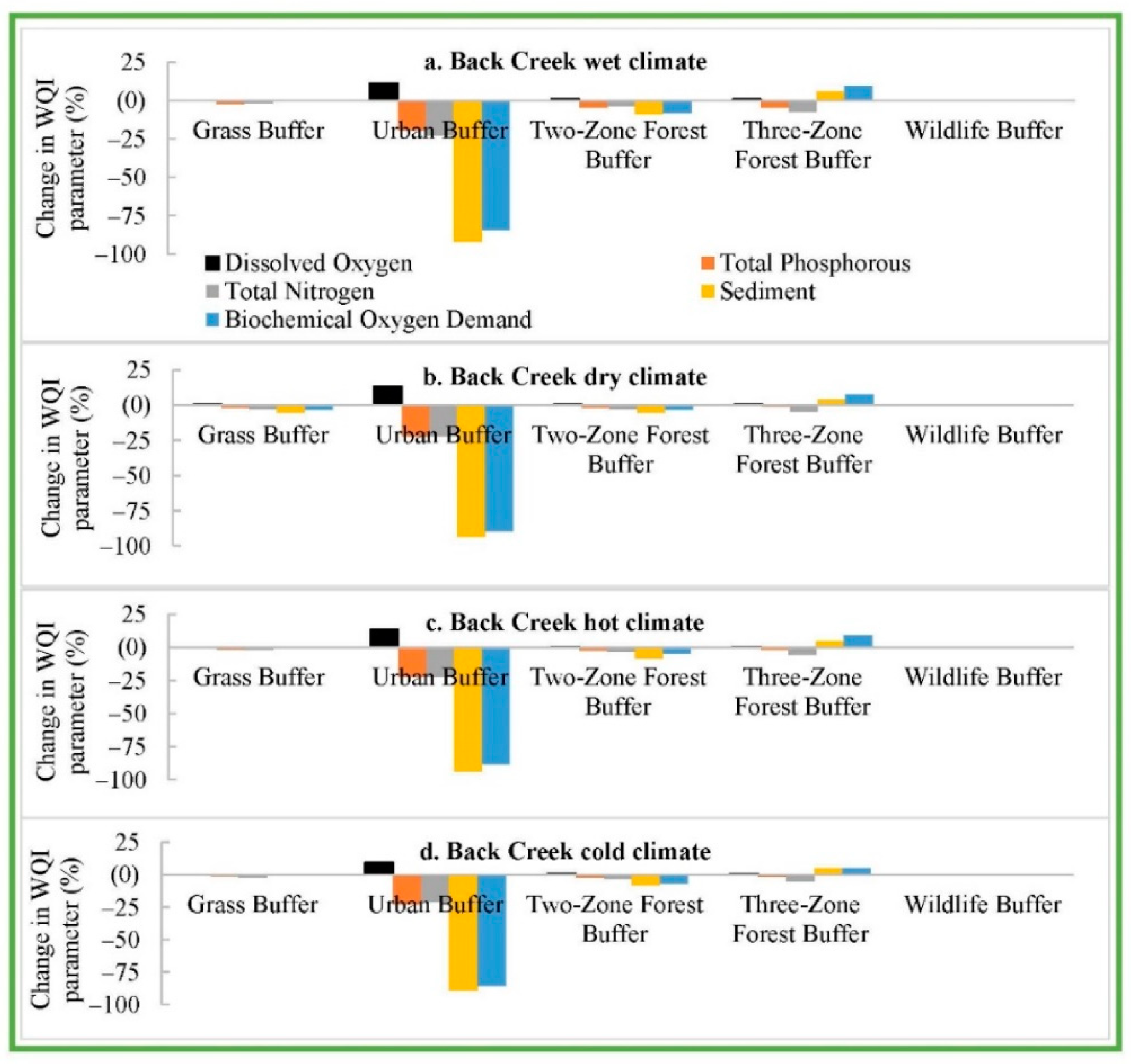
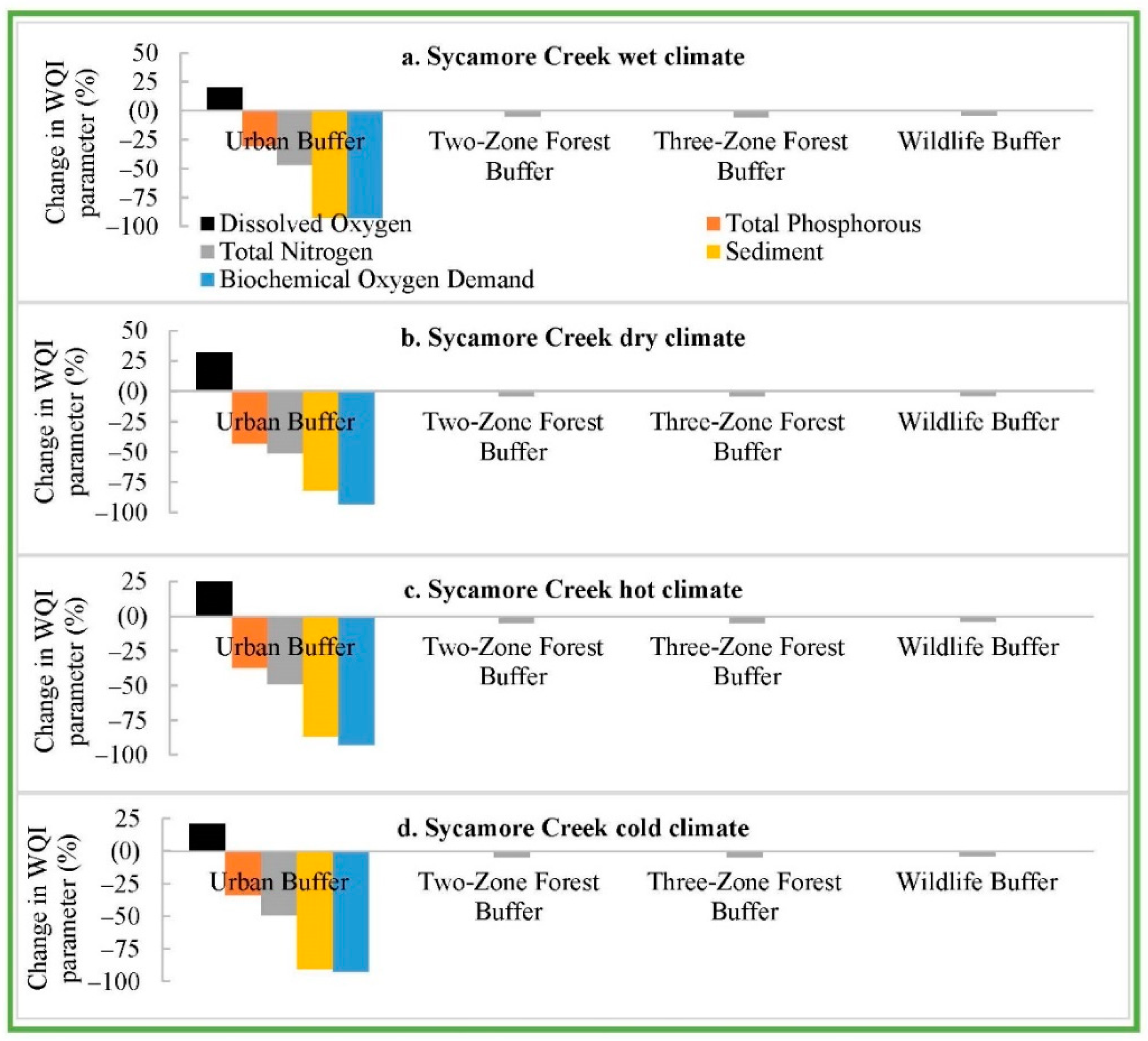
3.4. LASSO—Climate Projections and Sensitivity to WQI Parameters
4. Discussion
5. Conclusions
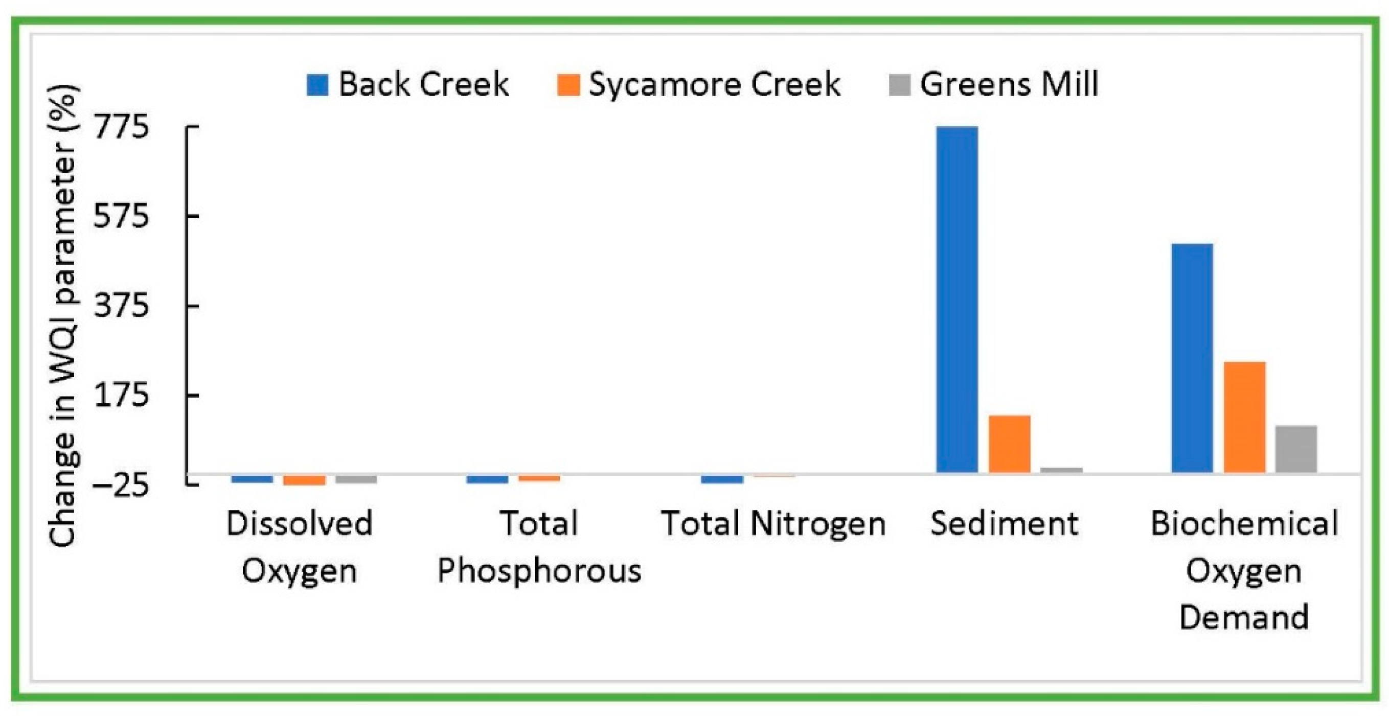
- The WQI parameter tradeoffs were watershed-specific and influenced by future extreme climates, suggesting a watershed-specific assessment.
- In terms of watershed ecosystem services, the optimal urban RBZ under contemporary climate reduced TP, TN, SD, and BD by 48%, 55%, 96%, and 99%, respectively, and raised dissolved oxygen by 10% with respect to the maximum values of No-RBZ in Sycamore Creek. The projected future extreme climate change significantly increased the projected SD and BD with respect to the current climate no-RBZ condition in Back Creek; however, the addition of an Urban RBZ resulted in reductions of SD and BD by 94% and 88%.
- Current models are transferrable to simulate RBZs along hydrologically connected aquatic systems of rivers, lakes, ponds, and wetlands in the U.S., from eastern to southeastern to the midwestern regions, yielding average to substantial quantities of non-point source pollutants into surface and ground waters by obtaining watershed-specific information, such as geographic database and spatial/temporal weather data. Current methods and findings are useful in assessing the effectiveness of RBZ policies in the Southeast U.S. and outside with similar watershed characteristics. For example, the methods can be useful for developing RBZ design policies to assess the effectiveness of the Comprehensive Conservation and Management Plan (2012–2022) of the Albemarle-Pamlico National Estuary Partnership (APNEP) [63]. Nationally, the outcomes can support the U.S. government’s various riparian restoration and preservation programs, including the USDA Conservation Reserve Program, which promotes the development of riparian buffers along streams [64].
- This study serves as the first step towards RBZ designs and holistic watershed management through a cross-disciplinary approach of eco-efficiency and sustainability [66].
Author Contributions
Funding
Informed Consent Statement
Data Availability Statement
Acknowledgments
Conflicts of Interest
Appendix A
LASSO Simulation


| Author (Year) | Riparian Buffer Designs | Summary |
|---|---|---|
| Jiang, et al. [68] | Proposed six RBZ designs: (i) 10 m grass, (ii) 15 m grass, (iii) 15 m deciduous trees, (iv) 30 m grass and trees, (v) 30 m grass and trees with trees harvested every 3 years, and (vi) 30 m grass and trees with grass harvested every year. | Evaluated watershed scale nutrient and sediment loads using soil and water assessment tool (SWAT) coupled with the riparian ecosystem management model (REMM). Reported reduction efficiencies of 76–78% for total nitrogen, 51–55% total phosphorus, and 68% sediment. Recommended flexible, farmer-preferred buffer design policies. |
| Jiang, et al. [62] | Proposed six RBZ designs: Design 1 (10 m zone 1 grass); Design 2 (15 m zone 1 grass); Design 3 (15 m zone 1 deciduous trees); Design 4 (6 m zone 1 grass, 19 m zone 2 deciduous trees, and 5 m zone 3 deciduous trees); Design 5 (6 m zone 1 grass, 19 m zone 2 deciduous trees harvested every 3 years, and 5 m zone 3 deciduous Trees); Design 6 (6 m zone 1 grass harvested every 3 years, 19 m zone 2 deciduous trees, and 5 m zone 3 deciduous trees). | Three crop rotations were also simulated using the SWAT coupled to the REMM. Reported annual total reduction rate of sediments and dissolved N at 90.8% and 91.9%. |
| Piscoya, et al. [69] | Reported a range of RBZ width from 7.6 m to 15.3 m for a small (2.10 km2) semiarid Brazilian watershed. | Determined RBZ width using a variable width equation for the incoming discharges, sediment loads, the slope, area, and annual soil loss. Concluded that the sediment yield time and hydrological data were important factors for determining the RBZ width. |
| Liu, et al. [70] | Created five RBZ designs: (i) Design 1 (10 m zone 1 of non-harvestable deciduous upper canopy forest next to the river + 20 m zone 2 of harvestable deciduous upper canopy forests in the middle + 20 m zone 3 of herbaceous perennials next to the field); (ii) Design 2 (10 m zone 1, 20 m zone 2); (iii) Design 3 (10 m zone 1); Design 4 (10 m zone 1, 10 m Zone 2); Design 5 (10 m zone 3 and 10 m zone 1). | Assessed impact of designs on water quality in a watershed in China using the Agricultural Non-Point Source Pollution Model (AnnAGNPS) and the REMM. Reported the removal efficiency of sediments from 85.7% to 90.8% and dissolved nitrogen in surface runoff from 85.4% to 91.9%. |
| Santin, et al. [71] | Reported the largest width value at 47 m and suggested the vegetation cover type as the single most relevant variable among soil type, mean nitrogen influent, and nitrogen removal effectiveness. | Proposed a method to estimate the riparian buffer width (the output) as a function of vegetation cover type, soil type, mean nitrogen influent, and nitrogen removal effectiveness (the inputs) in an agricultural watershed in Brazil using artificial neural networks (ANNs) and literature data. |
| Tomer, et al. [72] | Classified riparian sites into three groups according to runoff-contributing areas (the ratio of contributing area to buffer area): (i) high (potential to receive overland flow from large upslope areas); (ii) medium (wider than 10 m to provide a buffer-contributing area ratio of 0.02); (iii) low (narrow buffer, 10-m wide or less, provides the minimum recommended contributing area ratio of 0.02). | Proposed a geographic information system or GIS-based approach to identify riparian management alternatives in Iowa and Illinois using light detection and ranging (LiDAR) with high-resolution digital elevation models (DEMs). |
| Cardinali, et al. [73] | Compared four buffer designs in an experimental crop field of 200 m × 35 m: (i) 3 m wide grass buffer; (ii) 3 m grass with one tree row; (iii) 6 m grass with one tree row; (iv) 6 m grass with two tree rows in an experimental farm in Italy. | Evaluated the buffer impacts on soil quality parameters (soil organic matter, soil microbial functional diversity, and soil enzyme activities). Reported that the 3 m grass and 3 m grass with one tree row buffers produced the highest values of soil organic matter quality parameters. |
| Johnson and Buffler [74] | Presented unadjusted optimal buffer widths for four slope categories and three hydrologic soil groups—from 21 m (70 ft) for the lowest slope range of 0% to 5% and high surface roughness hydrologic group to 58 m (190 ft) for highest slope range of 15% to 25% and low surface roughness hydrologic group. | Proposed a protocol for buffer widths for water quality and wildlife habitat functions to accommodate Intermountain West landscape attributes (northern Utah and Nevada, eastern Oregon, southwestern Montana, and Wyoming). The unadjusted widths would be subsequently adjusted to account for the presence of other buffer variables, such as wetlands, surface water features, springs, significant sand and gravel aquifers, and very steep slopes. |
| Buffler [65] | Recommended RBZ width ranges required for removal of selected contaminants: 20 to > 40 m for N, 3 to > 10 m for sediment, >20 m for P (dissolved and particulate), 3 to >6 m for pathogens associated with sediments, and >9 m for pesticides particulates associated with sediment. | Conducted literature review on riparian buffer width for water quality parameters within the Intermountain West and literature in other physiographic regions of the United States. |
| Hairston-Strang [75] | Recommended a minimum width of 11 m (35 ft) and suggested 100 m (300 ft) and wider buffers for wildlife and biodiversity. | Provided general guidance for riparian forest buffer design and maintenance strategies. |
| Fox, et al. [76] | Used the minimum width of grass RBZ width from 6 to 9 m (20 to 30 ft) and forest RBZ width at 11 m (35 ft). | Provided guidance on design of a riparian buffer and selection of appropriate tree and grass species. |
| Fischer and Fischenich [13] | Provided RBZ width recommendations based on functions of water quality protection (5–30 m), riparian habitat (30 to 500 m), stream stabilization (10 to 20 m), flood attenuation (20 to 150 m), and detrital input (3 to 10 m). | Provided general recommendations for RBZ management, suggesting a diverse array of plant species in a range of site conditions. |
| Dosskey, et al. [77] | Recommended minimum RBZ width from 7.6 m to 9.1 m (25–30 ft) to filter sediment, up to 30.5 m (100 ft) to provide shade, shelter, and food for aquatic organisms, and variable widths for wildlife habitat dependent upon the desired species. | Recommended minimum acceptable RBZ width depending on site conditions, vegetation type, and landowner objectives. |
| Dosskey, et al. [78] | Proposed a general cropland riparian buffer design consisting of a 15 m (50 ft)-wide strip of grass, shrubs, and trees between the normal bank-full water level and cropland. | Suggested the design be adjusted to better suit specific landowner needs and site conditions. |
| Schultz, et al. [61] | Designed a multi-species RBZ system of a 20 m wide filter strip consisting of four or five rows of fast-growing trees planted closest to the stream, two shrub rows, and a 7 m wide strip of switchgrass next to the agricultural fields. | Designed the RBZ system along a Central Iowa stream and reported better soil stabilization, absorption of infiltrated water, and lower Nitrate-nitrogen concentrations (2 mg/L) as opposed to the levels in the adjacent agricultural fields over 12 mg/L. |
| Isenhart, et al. [79] | Designed a multi-species RBZ. The first 10 m wide zone contained four or five rows of rapidly growing trees, the second 4 m zone contained one or two rows of shrubs, and the third 7 m zone contained native, warm-season grasses. | Reported that the buffer strips reduced sediment and chemicals by trapping over 90% of the material. |
| Christian [80] | Created a 21.3 m tree-shrub-grass buffer zone with a 7.3 m wide strip of a native prairie grass, switchgrass, adjacent to fields under agronomic production in Iowa. In addition, designed a 67.0 m tree-shrub-grass buffer zone along the 45.7 m grass field to address the convex-concave slope. | Analyzed the performance of RBZs at reducing sediment delivery to streams using the chemicals, runoff and erosion from agricultural management systems (CREAMS) model and reported 42% sediment reduction. |
| Li, et al. [81] | Created five buffer designs (10 m grass; 15 m grass; 15 m trees; 6 m grass and 24 m trees; 30 m grass) in a watershed in Pennsylvania. Simulated the nutrients and sediment loads and explored the impacts of crop rotations using the REMM along with SWAT. | Additionally, developed dynamic optimization models to investigate the necessary payoffs for farmers and landowners to adopt RBZs, suggesting that higher adoptions would be achieved with flexible buffers. |
| Land Use | Crabtree Creek | Greens Mill Run |
|---|---|---|
| Urban (%) | 64.6 | 69.6 |
| Forested (%) | 30 | 21 |
| Grass/crop (%) | 4.1 | 9.4 |
| Precipitation (mm) | 1192.8 | 1299.2 |
| A. Back Creek KGE Parameter Calibration | ||||||
|---|---|---|---|---|---|---|
| Parameter Name | Description | Best Fit Value | Min. Value | Max. Value | T-Statistic | p-Value |
| A__GWQMN.gw | Threshold depth of water in the shallow aquifer required for return flow to occur | −933.08 | −1000 | 1000 | −23.7 | 0 |
| A__REVAPMN.gw | Threshold depth of water in the shallow aquifer for revap to occur | −559.04 | −750 | 750 | 3.67 | 0 |
| V__LAT_TTIME.HRU | Lateral flow travel time | 23.77 | 0 | 200 | -5.96 | 0 |
| A__GW_DELAY.gw | Ground water delay | −19.98 | −30 | 90 | −29.2 | 0 |
| V__CANMX.HRU (FRSE, FRSD, FRST only) | Maximum canopy storage | 9.11 | 0 | 25 | −16.78 | 0 |
| V__SLSOIL.HRU | Slope length for lateral subsurface flow | 2.37 | 0 | 150 | 2.66 | 0.01 |
| V__ALPHA_BF.gw | Baseflow alpha factor | 0.9 | 0 | 1 | 7.52 | 0 |
| V__ALPHA_BF_D.gw | Baseflow alfa factor for deep aquifer | 0.7 | 0 | 1 | −1.75 | 0.08 |
| V__ESCO.HRU | Soil evaporation compensation factor | 0.61 | 0.6 | 1 | 8.74 | 0 |
| R__CN2.mgt | Initial SCS runoff curve number for moisture condition II | 0.1 | −0.1 | 0.1 | 12.34 | 0 |
| A__RCHRG_DP.gw | Deep aquifer percolation fraction | 0.03 | −0.05 | 0.05 | −0.06 | 0.95 |
| V__GW_REVAP.gw | Ground water revap coefficient | 0.02 | 0.02 | 0.1 | −21.33 | 0 |
| R__SOL_AWC.sol | Available water capacity of the soil layer | 0.02 | −0.05 | 0.05 | 0.93 | 0.35 |
| B. Sycamore Creek NSE Parameter Calibration | ||||||
| A__REVAPMN.gw | Threshold depth of water in the shallow aquifer for revap to occur | 134.42 | −750 | 750 | 3.05 | 0 |
| A__GWQMN.gw | Threshold depth of water in the shallow aquifer required for return flow to occur | −60.77 | −1000 | 1000 | −3.48 | 0 |
| A__GW_DELAY.gw | Ground water delay | 29.03 | −30 | 90 | −0.39 | 0.7 |
| V__CANMX.HRU (FRSE, FRSD, FRST only) | Maximum canopy storage | 12.02 | 0 | 15 | −16.89 | 0 |
| V__SLSOIL.HRU | Slope length for lateral subsurface flow | 1.33 | 0 | 150 | −9.91 | 0 |
| V__LAT_TTIME.HRU | Lateral flow travel time | 1.01 | 0 | 14 | −11.24 | 0 |
| V__ALPHA_BF_D.gw | Baseflow alfa factor for deep aquifer | 1 | 1 | 1 | −0.17 | 0.87 |
| V__ESCO.HRU | Soil evaporation compensation factor | 0.94 | 0.6 | 1 | 123.2 | 0 |
| V__ALPHA_BF.gw | Baseflow alpha factor | 0.37 | 0 | 1 | 0.79 | 0.43 |
| R__CN2.mgt | Initial SCS runoff curve number for moisture condition II | 0.1 | −0.1 | 0.1 | 8.24 | 0 |
| V__GW_REVAP.gw | Ground water revap coefficient | 0.05 | 0.02 | 0.1 | −1.47 | 0.14 |
| R__SOL_AWC.sol | Available water capacity of the soil layer | 0.02 | −0.05 | 0.05 | −3.63 | 0 |
| A__RCHRG_DP.gw | Deep aquifer percolation fraction | 0.01 | −0.05 | 0.05 | −0.39 | 0.7 |
| Simulation Order | Location | Dataset (D) | RCP (E) | Timeframe (P) | Season (T) | Strategy (S) | Number of Options (D.E.P.T.S) |
|---|---|---|---|---|---|---|---|
| 1 | NC | LOCA (1) | RCP8.5 (1) | All three (3) | All five (5) | LASSO (1) | 15 |
| 2 | NC | BCSD (1) | RCP8.5 (1) | 2070–2099 (1) | Annual (1) | LASSO (1) | 1 |
| 3 | NC | LOCA (1) | RCP4.5 (1) | 2070–2099 (1) | Annual (1) | LASSO (1) | 1 |
| 4 | NC | LOCA (1) | RCP8.5 (1) | 2070–2099 (1) | Annual (1) | Four Corners (1) | 1 |
| 5 | NC | LOCA (1) | RCP8.5 (1) | 2070–2099 (1) | Annual (1) | Middle Corners (1) | 1 |
| 6 | NC | LOCA (1) | RCP8.5 (1) | 2070–2099 (1) | Annual (1) | Double Median (1) | 1 |
| 7 | VA | LOCA (1) | RCP8.5 (1) | 2070–2099 (1) | Annual (1) | LASSO (1) | 1 |
References
- USEPA. 2017 National Water Quality Inventory Report to Congress; U.S. Environmental Protection Agency: Washington, DC, USA, 2017. [Google Scholar]
- Chesters, G.; Schierow, L.-J. A primer on nonpoint pollution. J. Soil Water Conserv. 1985, 40, 9–13. [Google Scholar]
- Ghimire, S.R.; Johnston, J.M. Sustainability assessment of agricultural rainwater harvesting: Evaluation of alternative crop types and irrigation practices. PLoS ONE 2019, 14, e0216452. [Google Scholar] [CrossRef]
- Kalnay, E.; Cai, M. Impact of urbanization and land-use change on climate. Nature 2003, 423, 528–531. [Google Scholar] [CrossRef]
- Seto, K.C.; Güneralp, B.; Hutyra, L.R. Global forecasts of urban expansion to 2030 and direct impacts on biodiversity and carbon pools. Proc. Natl. Acad. Sci. USA 2012, 109, 16083–16088. [Google Scholar] [CrossRef] [PubMed] [Green Version]
- Vigiak, O.; Malagó, A.; Bouraoui, F.; Grizzetti, B.; Weissteiner, C.J.; Pastori, M. Impact of current riparian land on sediment retention in the Danube River Basin. Sustain. Water Qual. Ecol. 2016, 8, 30–49. [Google Scholar] [CrossRef]
- Mayer, P.M.; Reynolds, S.K., Jr.; McCutchen, M.D.; Canfield, T.J. Meta-analysis of nitrogen removal in riparian buffers. J. Environ. Qual. 2007, 36, 1172–1180. [Google Scholar] [CrossRef]
- Fischer, R.A.; Martin, C.O.; Fischenich, J. Improving riparian buffer strips and corridors for water quality and wildlife. In Proceedings of the International Conference on Riparian Ecology and Management in Multi-Land use Watersheds, Oregon, Portland, 28–31 August 2000. [Google Scholar]
- Cole, L.J.; Stockan, J.; Helliwell, R. Managing riparian buffer strips to optimise ecosystem services: A review. Agric. Ecosyst. Environ. 2020, 296, 106891. [Google Scholar] [CrossRef]
- Pachauri, R.K.; Allen, M.R.; Barros, V.R.; Broome, J.; Cramer, W.; Christ, R.; Church, J.A.; Clarke, L.; Dahe, Q.; Dasgupta, P. Climate Change 2014: Synthesis Report. Contribution of Working Groups I, II and III to the Fifth Assessment Report of the Intergovernmental Panel on Climate Change; IPCC: Geneva, Switzerland, 2014. [Google Scholar]
- Mander, Ü.; Hayakawa, Y.; Kuusemets, V. Purification processes, ecological functions, planning and design of riparian buffer zones in agricultural watersheds. Ecol. Eng. 2005, 24, 421–432. [Google Scholar] [CrossRef]
- USEPA. Riparian Buffer width, Vegetative Cover, and Nitrogen Removal Effectiveness: A Review of Current Science and Regulations; U.S. Environmental Protection Agency: Cincinnati, OH, USA, 2005. [Google Scholar]
- Fischer, R.A.; Fischenich, J.C. Design Recommendations for Riparian Corridors and Vegetated Buffer Strips; U.S. Army Corps of Engineers: Vicksburg, MS, USA, 2000. [Google Scholar]
- Valkama, E.; Usva, K.; Saarinen, M.; Uusi-Kämppä, J. A Meta-Analysis on Nitrogen Retention by Buffer Zones. J. Environ. Qual. 2019, 48, 270–279. [Google Scholar] [CrossRef] [Green Version]
- Blankenberg, A.-G.B.; Skarbøvik, E. Phosphorus retention, erosion protection and farmers’ perceptions of riparian buffer zones with grass and natural vegetation: Case studies from South-Eastern Norway. Ambio 2020, 49, 1838–1849. [Google Scholar] [CrossRef]
- Mayer, P.M.; Todd, A.H.; Okay, J.A.; Dwire, K.A. Introduction to the Featured Collection on Riparian Ecosystems & Buffers1. JAWRA J. Am. Water Resour. Assoc. 2010, 46, 207–210. [Google Scholar] [CrossRef]
- Vidon, P.; Allan, C.; Burns, D.; Duval, T.P.; Gurwick, N.; Inamdar, S.; Lowrance, R.; Okay, J.; Scott, D.; Sebestyen, S. Hot Spots and Hot Moments in Riparian Zones: Potential for Improved Water Quality Management1. JAWRA J. Am. Water Resour. Assoc. 2010, 46, 278–298. [Google Scholar] [CrossRef]
- Newbold, J.D.; Herbert, S.; Sweeney, B.W.; Kiry, P.; Alberts, S.J. Water Quality Functions of a 15-Year-Old Riparian Forest Buffer System1. JAWRA J. Am. Water Resour. Assoc. 2010, 46, 299–310. [Google Scholar] [CrossRef]
- Dewalle, D.R. Modeling Stream Shade: Riparian Buffer Height and Density as Important as Buffer Width1. JAWRA J. Am. Water Resour. Assoc. 2010, 46, 323–333. [Google Scholar] [CrossRef]
- Swanson, S.; Kozlowski, D.; Hall, R.; Heggem, D.; Lin, J. Riparian proper functioning condition assessment to improve watershed management for water quality. J. Soil Water Conserv. 2017, 72, 168–182. [Google Scholar] [CrossRef] [Green Version]
- Hoffmann, C.C.; Kjaergaard, C.; Uusi-Kämppä, J.; Hansen, H.C.B.; Kronvang, B. Phosphorus Retention in Riparian Buffers: Review of Their Efficiency. J. Environ. Qual. 2009, 38, 1942–1955. [Google Scholar] [CrossRef]
- Zhang, X.; Liu, X.; Zhang, M.; Dahlgren, R.A.; Eitzel, M. A Review of Vegetated Buffers and a Meta-analysis of Their Mitigation Efficacy in Reducing Nonpoint Source Pollution. J. Environ. Qual. 2010, 39, 76–84. [Google Scholar] [CrossRef]
- Uusi-Kämppä, J.; Braskerud, B.; Jansson, H.; Syversen, N.; Uusitalo, R. Buffer Zones and Constructed Wetlands as Filters for Agricultural Phosphorus. J. Environ. Qual. 2000, 29, 151–158. [Google Scholar] [CrossRef]
- Spruill, T. Effectiveness of riparian buffers in controlling ground-water discharge of nitrate to streams in selected hydrogeologic settings of the North Carolina Coastal Plain. Water Sci. Technol. 2004, 49, 63–70. [Google Scholar] [CrossRef]
- Cooper, J.R.; Gilliam, J.W.; Daniels, R.B.; Robarge, W.P. Riparian Areas as Filters for Agricultural Sediment1. Soil Sci. Soc. Am. J. 1987, 51, 416–420. [Google Scholar] [CrossRef]
- Daniels, R.B.; Gilliam, J.W. Sediment and Chemical Load Reduction by Grass and Riparian Filters. Soil Sci. Soc. Am. J. 1996, 60, 246–251. [Google Scholar] [CrossRef]
- Schmitt, T.J.; Dosskey, M.G.; Hoagland, K.D. Filter Strip Performance and Processes for Different Vegetation, Widths, and Contaminants. J. Environ. Qual. 1999, 28, 1479–1489. [Google Scholar] [CrossRef] [Green Version]
- Dillaha, T.A.; Reneau, R.; Mostaghimi, S.; Lee, D. Vegetative Filter Strips for Agricultural Nonpoint Source Pollution Control. Trans. ASAE 1989, 32, 0513–0519. [Google Scholar] [CrossRef]
- Lowrance, R.; Altier, L.S.; Newbold, J.D.; Schnabel, R.R.; Groffman, P.M.; Denver, J.M.; Correll, D.L.; Gilliam, J.W.; Robinson, J.L.; Brinsfield, R.B.; et al. Water Quality Functions of Riparian Forest Buffers in Chesapeake Bay Watersheds. Environ. Manag. 1997, 21, 687–712. [Google Scholar] [CrossRef]
- Weller, D.E.; Baker, M.; Jordan, T.E. Effects of riparian buffers on nitrate concentrations in watershed discharges: New models and management implications. Ecol. Appl. 2011, 21, 1679–1695. [Google Scholar] [CrossRef]
- Lyons, J.; Thimble, S.W.; Paine, L.K. Grass versus trees: Managing riparian areas to benefit streams of central north America. JAWRA J. Am. Water Resour. Assoc. 2000, 36, 919–930. [Google Scholar] [CrossRef]
- Sweeney, B.W.; Newbold, J.D. Streamside Forest Buffer Width Needed to Protect Stream Water Quality, Habitat, and Organisms: A Literature Review. JAWRA J. Am. Water Resour. Assoc. 2013, 50, 560–584. [Google Scholar] [CrossRef]
- USEPA. Impaired Waters and TMDLs. Available online: https://www.epa.gov/tmdl/overview-identifying-and-restoring-impaired-waters-under-section-303d-cwa (accessed on 29 September 2020).
- USGPO. Clean Water Act (Federal Water Pollution Control Act). 2020, [Chapter 758 of the 80th Congress] [33 U.S.C. 1251 et seq.]. Available online: https://www.govinfo.gov/app/collection/comps/c/%7B%22pageSize%22%3A%2220%22%7D (accessed on 24 August 2021).
- Ghimire, S.R.; Johnston, J.M. Impacts of domestic and agricultural rainwater harvesting systems on watershed hydrology: A case study in the Albemarle-Pamlico river basins (USA). Ecohydrol. Hydrobiol. 2013, 13, 159–171. [Google Scholar] [CrossRef]
- Ghimire, S.R.; Johnston, J.M.; Ingwersen, W.W.; Hawkins, T.R. Life Cycle Assessment of Domestic and Agricultural Rainwater Harvesting Systems. Environ. Sci. Technol. 2014, 48, 4069–4077. [Google Scholar] [CrossRef]
- Johnston, J.; McGarvey, D.; Barber, M.C.; Laniak, G.; Babendreier, J.; Parmar, R.; Wolfe, K.; Kraemer, S.R.; Cyterski, M.; Knightes, C.; et al. An integrated modeling framework for performing environmental assessments: Application to ecosystem services in the Albemarle-Pamlico basins (NC and VA, USA). Ecol. Model. 2011, 222, 2471–2484. [Google Scholar] [CrossRef]
- APNEP. The Albemarle-Pamlico National Estuary Partnership. Available online: https://apnep.nc.gov/our-estuary/fast-facts (accessed on 6 May 2021).
- Survey, U.G. MRLC Consortium—National Land Cover Database 2001. Available online: https://www.usgs.gov/centers/eros/science/national-land-cover-database?qt-science_center_objects=0#qt-science_center_objects (accessed on 24 February 2021).
- USDA. Land Use—Cropland Data Layer (Agricultural). Available online: https://nassgeodata.gmu.edu/CropScape/ (accessed on 24 February 2021).
- Cunningham, K.; Stuhlinger, C.; Liechty, H. Riparian Buffers: Types and Establishment Methods; University of Arkansas, Division of Agriculture Cooperative Extension: Fayetteville, AR, USA, 2009; Available online: https://www.landcan.org/pdfs/rip%20buffer%20types.pdf (accessed on 24 August 2021).
- USEPA. HAWQS Version 1.2. Available online: https://new.hawqs.tamu.edu/#/ (accessed on 30 September 2020).
- USDA Agricultural Research Service (USDA-ARS). Texas AgriLife Research Soil & Water Assessment Tool (SWAT). Available online: https://swat.tamu.edu (accessed on 14 March 2020).
- Daly, C.; Neilson, R.P.; Phillips, D.L. A statistical-topographic model for mapping climatological precipitation over mountainous terrain. J. Appl. Meteorol. Climatol. 1994, 33, 140–158. [Google Scholar] [CrossRef] [Green Version]
- Arnold, J.; Kiniry, J.; Srinivasan, R.; Williams, J.; Haney, E.; Neitsch, S. SWAT 2012 Input/Output Documentation; Texas Water Resources Institute: College Station, TX, USA, 2013. [Google Scholar]
- TAMU. SWAT Executables. Available online: https://swat.tamu.edu/software/swat-executables/ (accessed on 26 October 2020).
- Winchell, M.; Srinivasan, R.; Di Luzio, M.; Arnold, J. ArcSWAT Interface for SWAT 2012; Texas A&M University: College Station, TX, USA, 2013. [Google Scholar]
- Neitsch, S.L.; Arnold, J.G.; Kiniry, J.R.; Williams, J.R. Soil and Water Assessment Tool Theoretical Documentation Version 2009; Texas Water Resources Institute: College Station, TX, USA, 2011. [Google Scholar]
- Waidler, D.; White, M.; Steglich, E.; Wang, S.; Williams, J.; Jones, C.; Srinivasan, R. Conservation Practice Modeling Guide for SWAT and APEX; Texas Water Resources Institute: College Station, TX, USA, 2011. [Google Scholar]
- USDA. State Soil Geographic Data. Available online: https://sdmdataaccess.nrcs.usda.gov/ (accessed on 5 March 2021).
- TAMU. HAWQS User Guide; Texas A&M University: College Station, TX, USA, 2019. [Google Scholar]
- Abbaspour, C.K. SWAT calibration and uncertainty programs. A User Manual. Eawag Zur. Switz. 2015, 20, 1–100. [Google Scholar]
- Moriasi, D.N.; Arnold, J.G.; Van Liew, M.W.; Bingner, R.L.; Harmel, R.D.; Veith, T.L. Model Evaluation Guidelines for Systematic Quantification of Accuracy in Watershed Simulations. Trans. ASABE 2007, 50, 885–900. [Google Scholar] [CrossRef]
- USEPA. About LASSO. Available online: https://www.epa.gov/gcx/about-lasso (accessed on 2 December 2020).
- USEPA. A Systematic Approach for Selecting Climate Projections to Inform Regional Impact Assessments; U.S. Environmental Protection Agency: Washington, DC, USA, 2020. [Google Scholar]
- IPCC. What is a GCM? Available online: https://www.ipcc-data.org/guidelines/pages/gcm_guide.html (accessed on 17 February 2021).
- WCRP. WCRP Coupled Model Intercomparison Project (CMIP). Available online: https://www.wcrp-climate.org/wgcm-cmip (accessed on 17 February 2021).
- Van Vuuren, D.P.; Edmonds, J.; Kainuma, M.; Riahi, K.; Thomson, A.; Hibbard, K.; Hurtt, G.C.; Kram, T.; Krey, V.; Lamarque, J.-F.; et al. The representative concentration pathways: An overview. Clim. Chang. 2011, 109, 5–31. [Google Scholar] [CrossRef]
- Quinn, J.D.; Hadjimichael, A.; Reed, P.M.; Steinschneider, S. Can Exploratory Modeling of Water Scarcity Vulnerabilities and Robustness Be Scenario Neutral? Earth’s Futur. 2020, 8, 001650. [Google Scholar] [CrossRef]
- NCDENR. Albemarle-Pamlico Baseline Water Quality Monitoring Data Summary; North Carolina Department of Environment Health, and Natural Resources: Mooresville, NC, USA, 1992. [Google Scholar]
- Schultz, R.C.; Collettil, J.P.; Isenhart, T.M.; Simpkins, W.W.; Mize, C.W.; Thompson, M.L. Design and placement of a multi-species riparian buffer strip system. Agrofor. Syst. 1995, 29, 201–226. [Google Scholar] [CrossRef]
- Jiang, F.; Gall, H.E.; Veith, T.L.; Cibin, R.; Drohan, P.J. Assessment of riparian buffers’ effectiveness in controlling nutrient and sediment loads as a function of buffer design, site characteristics and upland loadings. In Proceedings of the 2019 ASABE Annual International Meeting, Boston, MA, USA, 7–10 July 2019; p. 1. [Google Scholar]
- APNEP. Comprehensive Conservation and Management Plan (2012–2022); Albemarle-Pamlico National Estuary Partnership: Columbia, NC, USA, 2012. [Google Scholar]
- USDA. Conservation Reserve Enhancement Program. Available online: https://www.fsa.usda.gov/programs-and-services/conservation-programs/conservation-reserve-enhancement/index (accessed on 7 May 2021).
- Johnson, C.W.; Buffler, S. Riparian Buffer Design Guidelines for Water Quality and Wildlife Habitat Functions on Agricultural Landscapes in the Intermountain West; U.S. Department of Agriculture, Forest Service, North Central Forest Experiment Station: Fort Collins, CO, USA, 2008; Volume 203, p. 53. [Google Scholar]
- Ghimire, S.R.; Johnston, J.M. A modified eco-efficiency framework and methodology for advancing the state of practice of sustainability analysis as applied to green infrastructure. Integr. Environ. Assess. Manag. 2017, 13, 821–831. [Google Scholar] [CrossRef] [Green Version]
- USEPA. Water Reuse Research. Available online: https://www.epa.gov/water-research/water-reuse-research (accessed on 8 December 2020).
- Jiang, F.; Preisendanz, H.E.; Veith, T.L.; Cibin, R.; Drohan, P.J. Riparian buffer effectiveness as a function of buffer design and input loads. J. Environ. Qual. 2020, 49, 1599–1611. [Google Scholar] [CrossRef]
- Piscoya, V.C.; Singh, V.P.; Cantalice, J.R.B.; Guerra, S.M.S.; Filho, M.C.; Ribeiro, C.D.S.; Filho, R.N.D.A.; Da Luz, E.L.P. Riparian Buffer Strip Width Design in Semiarid Watershed Brazilian. J. Exp. Agric. Int. 2018, 23, 1–7. [Google Scholar] [CrossRef]
- Liu, C.; Wu, J.; Clausen, J.; Lei, T.; Yang, X. Impact of Riparian Buffer Design on Water Quality in the Jinghe Catchment, China. In Proceedings of the 2018 ASABE Annual International Meeting, Detroit, MI, USA; 2018; p. 1. [Google Scholar]
- Santin, F.; da Silva, R.; Grzybowski, J. Artificial neural network ensembles and the design of performance-oriented riparian buffer strips for the filtering of nitrogen in agricultural catchments. Ecol. Eng. 2016, 94, 493–502. [Google Scholar] [CrossRef]
- Tomer, M.D.; Boomer, K.M.B.; Porter, S.A.; Gelder, B.K.; James, D.E.; McLellan, E. Agricultural Conservation Planning Framework: 2. Classification of Riparian Buffer Design Types with Application to Assess and Map Stream Corridors. J. Environ. Qual. 2015, 44, 768–779. [Google Scholar] [CrossRef] [PubMed] [Green Version]
- Cardinali, A.; Carletti, P.; Nardi, S.; Zanin, G. Design of riparian buffer strips affects soil quality parameters. Appl. Soil Ecol. 2014, 80, 67–76. [Google Scholar] [CrossRef]
- Buffler, S. Riparian Buffer Design Guidelines for Water Quality and Wildlife Habitat Functions on Agricultural Landscapes in the Intermountain West: Appendix C; Gen. Tech. Rep. RMRS-GTR-203; U.S. Department of Agriculture, Forest Service, Rocky Mountain Research Station: Fort Collins, CO, USA, 2008; 59p. [Google Scholar]
- Hairston-Strang, A. Riparian Forest Buffer Design and Maintenance; Maryland Department of Natural Resources Forest Service: Carney, MD, USA, 2005. [Google Scholar]
- Fox, A.; Franti, T.G.; Josiah, S.J.; Kucera, M. G05-1557 Planning Your Riparian Buffer: Design and Plant Selection; Institute of Agriculture and Natural Resources, University of Nebraska-Lincoln: Lincoln, NE, USA, 2005. [Google Scholar]
- Dosskey, M.G.; Schultz, R.C.; Isenhart, T.M. How to Design a Riparian Buffer for Agricultural Land; Iowa State University: Ames, IA, USA, 1997. [Google Scholar]
- Dosskey, M.G.; Schultz, R.C.; Isenhart, T.M. A Riparian Buffer Design for Cropland; Iowa State University: Ames, IA, USA, 1997; p. 6. [Google Scholar]
- Isenhart, T.M.; Schultz, R.C.; Colletti, P.J. Design, Function, and Management of Multi-Species Riparian Buffer Strip Systems; Iowa State University: Ames, IA, USA, 1995. [Google Scholar]
- Christian, M.F. Application of the CREAMS Model to Simulate Performance of Riparian tree Buffer Strips: Implications for Buffer Strip Design; Iowa State University: Ames, IA, USA, 2018. [Google Scholar]
- Li, X.; Zipp, K.Y.; Jiang, F.; Veith, T.L.; Gall, H.E.; Royer, M.; Brooks, R.; Zikatanov, L.T.; Shortle, J.S. Integrated Assessment Modeling for Design of Riparian Buffer Systems and Incentives for Adoption. Available online: https://cpb-us-e1.wpmucdn.com/blogs.cornell.edu/dist/1/8608/files/2019/03/Li-et-al-2lpdbnu.pdf (accessed on 24 August 2021).


| RBZ Type | Average Width (m) | Description |
|---|---|---|
| Grass Buffer | 8 | This buffer consists only of grasses and forbs and is typically used along small streams and other drainages that flow through crop fields and pastures. The literature suggested buffer width is 6.1 m to 9.1 m. |
| Three-Zone Forest Buffer | 34 | This buffer consists of three zones: zone 1 (undisturbed forest), ranging in width from 4.6–9.1 m, contains trees along the edge of the stream; zone 2 (managed forest), ranging in width from 9.1–30.5 m, filters sediment that passes through zone 3 and absorbs nutrients while providing wildlife habitat; zone 3 (runoff control), 6.1–9.1 m wide, is usually a grass strip. The literature suggested that the minimum total buffer width on each side of a stream is 15.2–30.5 m but should be wider with increasing slope. |
| Two-Zone Forest Buffer | 27 | A two-zone forest buffer would simply be a modification to the three-zone forest buffer, where the grass zone (zone 3) would not be established. |
| Urban Buffer | 23 | This buffer consists of low-, medium-, and high-density residential land use types. The buffers can be used to teach users (homeowners and developers) about the RBZ’s water quality benefits. The literature suggested buffer width is 15.2–30.5 m. |
| Wildlife Buffer | 46 | This buffer consists of evergreen forest. A wildlife buffer is usually wider, to better function as a travel corridor and connector between larger tracts of forest. Suggested buffer width is up to 91.4 m. |
| Naturalized Buffer | 23 | This buffer consists of forested wetlands. This is an inexpensive natural buffer that can still effectively intercept runoff. Existing vegetation can be supplemented by interplanting tree and shrub seedlings. The literature suggested buffer width is 15.2–30.5 m. |
| RBZ Width Variation Scenario (Si) (i = 0 to 8) | RBZ Vegetation (Vi) | |||||
|---|---|---|---|---|---|---|
| Grass Buffer | Urban Buffer | Two-Zone Forest Buffer | Three-Zone Forest Buffer | Wildlife Buffer | Naturalized Buffer | |
| 0.0 × baseline width (S0) (No-RBZ) | 0 | 0 | 0 | 0 | 0 | 0 |
| 0.25 × baseline width (S1) | 2 | 6 | 7 | 9 | 11 | 6 |
| 0.50 × baseline width (S2) | 4 | 11 | 13 | 17 | 23 | 11 |
| 0.75 × baseline width (S3) | 6 | 17 | 20 | 26 | 34 | 17 |
| Baseline (1.0) RBZ width (S4) | 8 | 23 | 27 | 34 | 46 | 23 |
| 1.25 × baseline width (S5) | 10 | 29 | 33 | 43 | 57 | 29 |
| 1.50 × baseline width (S6) | 11 | 34 | 40 | 51 | 69 | 34 |
| 1.75 × baseline width (S7) | 13 | 40 | 47 | 60 | 80 | 40 |
| 2.0 × baseline width (S8) | 15 | 46 | 53 | 69 | 91 | 46 |
| Watershed | Stream Length (km) | Area (km2) | Population Density (People/km2) | Elevation Range (m) | Precipitation (cm) | Urban RBZ | Grass RBZ | Two-Zone Forest RBZ | * Three-Zone Forest RBZ | Wildlife RBZ | Naturalized RBZ |
|---|---|---|---|---|---|---|---|---|---|---|---|
| Back Creek | 40.0 | 152 | 100 | 305–646 | 106 | LMDR (19%) | Hay (7%) | EF/DF (74%) | EF/DF (74%) | EF (4%) | NA |
| Sycamore Creek | 12.1 | 41.7 | 600 | 74–136 | 111 | LMHDR (51%) | NA | EF/DF (49%) | EF/DF (49%) | EF (23%) | NA |
| Greens Mill Run | 22.9 | 34.7 | 900 | 0–46 | 127 | LMHDR (70%) | Range-Brush (4%) | EF (8%) | EF (8%) | EF (8%) | FW (13%) |
| Watershed | PBIAS | NSE | KGE | Average Flow (Observed) (m3/s) | Calibration Period |
|---|---|---|---|---|---|
| Back Creek | −3.90% | 0.83 | 0.91 | 1.92 (1.85) | 1983–2018 |
| Crabtree Creek (Sycamore Creek) | 3.80% | 0.87 | 0.85 | 3.75 (3.9) | 1988–2018 |
| Back Creek Watershed Baseline RBZs: All Values in mg/L | |||||||
|---|---|---|---|---|---|---|---|
| Water Quality Indicator Parameter | No-RBZ | Grass Buffer | Urban Buffer | Two-Zone Forest Buffer | Three-Zone Forest Buffer | Wildlife Buffer | Naturalized Buffer |
| Dissolved Oxygen | 9.6 | 9.6 | 10.0 | 9.7 | 9.7 | 9.6 | NA |
| Total Phosphorous | 0.2 | 0.2 | 0.1 | 0.2 | 0.2 | 0.2 | NA |
| Total Nitrogen | 2.0 | 2.0 | 1.4 | 2.0 | 1.9 | 2.0 | NA |
| Sediment Concentration | 12.7 | 12.3 | 3.9 | 10.1 | 11.2 | 12.7 | NA |
| Biochemical Oxygen Demand | 0.5 | 0.5 | 0.2 | 0.3 | 0.3 | 0.5 | NA |
| Sycamore Creek Watershed Baseline RBZs: All values in mg/L | |||||||
| Water Quality Indicator Parameter | No-RBZ | Grass Buffer | Urban Buffer | Two-Zone Forest Buffer | Three-Zone Forest Buffer | Wildlife Buffer | Naturalized Buffer |
| Dissolved Oxygen | 3.7 | NA | 4.1 | 3.7 | 3.7 | 3.7 | NA |
| Total Phosphorous | 0.2 | NA | 0.1 | 0.2 | 0.2 | 0.2 | NA |
| Total Nitrogen | 1.3 | NA | 0.7 | 1.3 | 1.3 | 1.3 | NA |
| Sediment Concentration | 19.3 | NA | 1.9 | 19.3 | 19.4 | 19.3 | NA |
| Biochemical Oxygen Demand | 0.5 | NA | 0.0 | 0.5 | 0.5 | 0.5 | NA |
| Greens Mill Run Watershed Baseline RBZs: All values in mg/L | |||||||
| Water Quality Indicator Parameter | No-RBZ | Grass Buffer | Urban Buffer | Two-Zone Forest Buffer | Three-Zone Forest Buffer | Wildlife Buffer | Naturalized Buffer |
| Dissolved Oxygen | 6.8 | 6.8 | 7.4 | 6.8 | 6.8 | 6.8 | 6.8 |
| Total Phosphorous | 0.4 | 0.4 | 0.4 | 0.4 | 0.4 | 0.4 | 0.4 |
| Total Nitrogen | 3.3 | 3.3 | 2.2 | 3.3 | 3.3 | 3.3 | 3.3 |
| Sediment Concentration | 61.0 | 60.9 | 26.2 | 61.0 | 61.0 | 61.0 | 60.9 |
| Biochemical Oxygen Demand | 2.2 | 2.2 | 1.1 | 2.2 | 2.2 | 2.2 | 2.2 |
| Climate Code | Climate Projection Scenario Name | Virginia | North Carolina | ||
|---|---|---|---|---|---|
| Annual Precipitation Change, ΔP (%) | Annual Air Temperature Change, ΔT (°C) | Δ P (%) | Δ T (°C) | ||
| Hot | Hadley Centre Global Environment Model version 2-Carbon Cycle (HadGEM2-CC) | 6.8 | 6.3 | 5.1 | 5.7 |
| Cold | Russian Institute for Numerical Mathematics Climate Model Version 4 (inmcm4) | −0.2 | 2.7 | −1.3 | 2.4 |
| Dry | Flexible Global Ocean–Atmosphere–Land System Model, Grid-point Version 2 (FGOALS-g2) | −3.2 | 5.4 | −10 | 5 |
| Wet | Max Planck Institute for Meteorology Earth System Model Mix Resolution (MPI-ESM-MR) | 23 | 4 | 19.5 | 3.8 |
Publisher’s Note: MDPI stays neutral with regard to jurisdictional claims in published maps and institutional affiliations. |
© 2021 by the authors. Licensee MDPI, Basel, Switzerland. This article is an open access article distributed under the terms and conditions of the Creative Commons Attribution (CC BY) license (https://creativecommons.org/licenses/by/4.0/).
Share and Cite
Ghimire, S.R.; Corona, J.; Parmar, R.; Mahadwar, G.; Srinivasan, R.; Mendoza, K.; Johnston, J.M. Sensitivity of Riparian Buffer Designs to Climate Change—Nutrient and Sediment Loading to Streams: A Case Study in the Albemarle-Pamlico River Basins (USA) Using HAWQS. Sustainability 2021, 13, 12380. https://doi.org/10.3390/su132212380
Ghimire SR, Corona J, Parmar R, Mahadwar G, Srinivasan R, Mendoza K, Johnston JM. Sensitivity of Riparian Buffer Designs to Climate Change—Nutrient and Sediment Loading to Streams: A Case Study in the Albemarle-Pamlico River Basins (USA) Using HAWQS. Sustainability. 2021; 13(22):12380. https://doi.org/10.3390/su132212380
Chicago/Turabian StyleGhimire, Santosh R., Joel Corona, Rajbir Parmar, Gouri Mahadwar, Raghavan Srinivasan, Katie Mendoza, and John M. Johnston. 2021. "Sensitivity of Riparian Buffer Designs to Climate Change—Nutrient and Sediment Loading to Streams: A Case Study in the Albemarle-Pamlico River Basins (USA) Using HAWQS" Sustainability 13, no. 22: 12380. https://doi.org/10.3390/su132212380
APA StyleGhimire, S. R., Corona, J., Parmar, R., Mahadwar, G., Srinivasan, R., Mendoza, K., & Johnston, J. M. (2021). Sensitivity of Riparian Buffer Designs to Climate Change—Nutrient and Sediment Loading to Streams: A Case Study in the Albemarle-Pamlico River Basins (USA) Using HAWQS. Sustainability, 13(22), 12380. https://doi.org/10.3390/su132212380