A Deep Learning Approach to Assist Sustainability of Demersal Trawling Operations

Abstract

Bycatch in demersal trawl fisheries challenges their sustainability despite the implementation of the various gear technical regulations. A step towards extended control over the catch process can be established through a real-time catch monitoring tool that will allow fishers to react to unwanted catch compositions. In this study, for the first time in the commercial demersal trawl fishery sector, we introduce an automated catch description that leverages state-of-the-art region based convolutional neural network (Mask R-CNN) architecture and builds upon an in-trawl novel image acquisition system. The system is optimized for applications in Nephrops fishery and enables the classification and count of catch items during fishing operation. The detector robustness was improved with augmentation techniques applied during training on a custom high-resolution dataset obtained during extensive demersal trawling. The resulting algorithms were tested on video footage representing both the normal towing process and haul-back conditions. The algorithm obtained an F-score of 0.79. The resulting automated catch description was compared with the manual catch count showing low absolute error during towing. Current practices in demersal trawl fisheries are carried out without any indications of catch composition nor whether the catch enters the fishing gear. Hence, the proposed solution provides a substantial technical contribution to making this type of fishery more targeted, paving the way to further optimization of fishing activities aiming at increasing target catch while reducing unwanted bycatch.

1. Introduction

Commercial demersal trawl fisheries are defined as mixed due to the high presence of co-habiting species in the catch, resulting in high catch rates of non-target sizes and individuals, referred to as bycatch [1]. In a quota-regulated management system, the commercial species and sizes can also be considered a bycatch if the individual vessel does not have quota available for a given species. Thus, the actual bycatch definition depends on fishery type and the area of fishing [2]. To mitigate catch and subsequent discard of unwanted species and sizes, ambitious management plans such as the EU Common Fisheries Policy landing obligation have been implemented, forcing fishers to declare all catches of listed species and count them against their quota [3]. The management plans are combined with technical regulations aiming at improving the gears size and species selectivity through mesh size regulations, trawl modifications and bycatch reduction devices. Despite these measures, catch of unwanted sizes and species still challenge these fisheries [2,4]. Indeed, such catch-quota systems as the landing obligation provide an incentive and not a tool to minimize unwanted catches. Additionally, available technical measures are not able to provide information on the ongoing catch; hence, catch composition can only be discovered when the fishing gear is lifted on board the vessel [5].

Recent developments in underwater imaging systems can help bring traditional demersal trawl fisheries into the digital age by enabling catch monitoring during fishing operations. Such systems are indeed crucial to overcome the challenges the demersal trawl fisheries face. The possibility to monitor the catch inside the trawl during fishing can provide valuable information and act as a decision support tool for fishers [6]. In-trawl camera systems are being introduced in pelagic fisheries [7,8,9,10] and demersal fisheries [6]; however, these systems have been, so far, used for scientific monitoring purpose only.

The developed catch monitoring methods are associated with extensive storage and manual processing of video recordings. To become an efficient decision support tool, these systems require automated processing of the data. Recently, automated processing of the data obtained by video cameras has become more common in various industries, and fisheries are not an exception. Several studies describe automated fish detection and classification commonly performed with the aid of deep learning models application [11,12,13,14,15]. These studies demonstrate that the deep learning models for objects detection and classification are efficient tools for processing the on-board as well as underwater collected recordings of the catch. The deep learning ability to “learn” the object features given the annotated data makes it a powerful tool for solving complex image analysis tasks. The traditional computer vision approaches require preliminary object features engineering for each specific task, which limits these methods’ efficient application to the real-world data [16].

However, the underwater video recordings, especially, are always challenged by poor visibility conditions [12,17]. Additionally, in the specific application of catch monitoring system in demersal trawls, more prominent occlusion conditions can limit the camera field of view due to sediment resuspension during gear towing [18,19]. Thus, acquisition of poor video recordings in bottom trawl applications can prevent quality data collection and hence hamper automated processing.

In this study, we demonstrate the successful automated processing of the catch based on the data collected during Nephrops-directed demersal trawling using a novel in-trawl image acquisition system, which helps to resolve the limitations caused by sediment mobilization [20]. We hypothesize that the quality of the collected data using the novel system is sufficient for developing an algorithm for automated catch description. With the described method, we aim at closing a gap in the demersal trawling operations non-transparency and enable fishers to monitor and hence have a better control over the catch building process during fishing operations. To test the hypothesis, we fine-tune a pre-trained convolutional neural network (CNN), specifically, the region based CNN-Mask R-CNN model [21], with the aid of several augmentation techniques aiming at improving model robustness by increasing the variability in training data. The trained detector was then coupled with the tracking algorithm to count the detected objects. The known behavior aspects during trawling of fish and Nephrops (Nephrops norvegicus, Linnaeus, 1758) were considered while tuning the Simple Online and Realtime Tracking (SORT) algorithm [22]. The resulting composite algorithm was tested against two types of videos depicting normal towing conditions (having low object occlusion and stable observation section) and the haul-back phase when the camera’s occlusion rate is higher and the observation section is less stable. We assessed the performances of the algorithm in classifying demersal trawl catches into four categories and against the total counts per category. Automated catch count was also compared with the actual catch count. The system shows good performances and, when further developed, can help fishers to comply with present management plans, preserving fisheries economic and ecological sustainability by enabling skippers to automatically monitor the catch during fishing operation and to react to the presence of unwanted catch by either interrupting the fishing operation or relocating to avoid the bycatch.

2. Methods and Materials

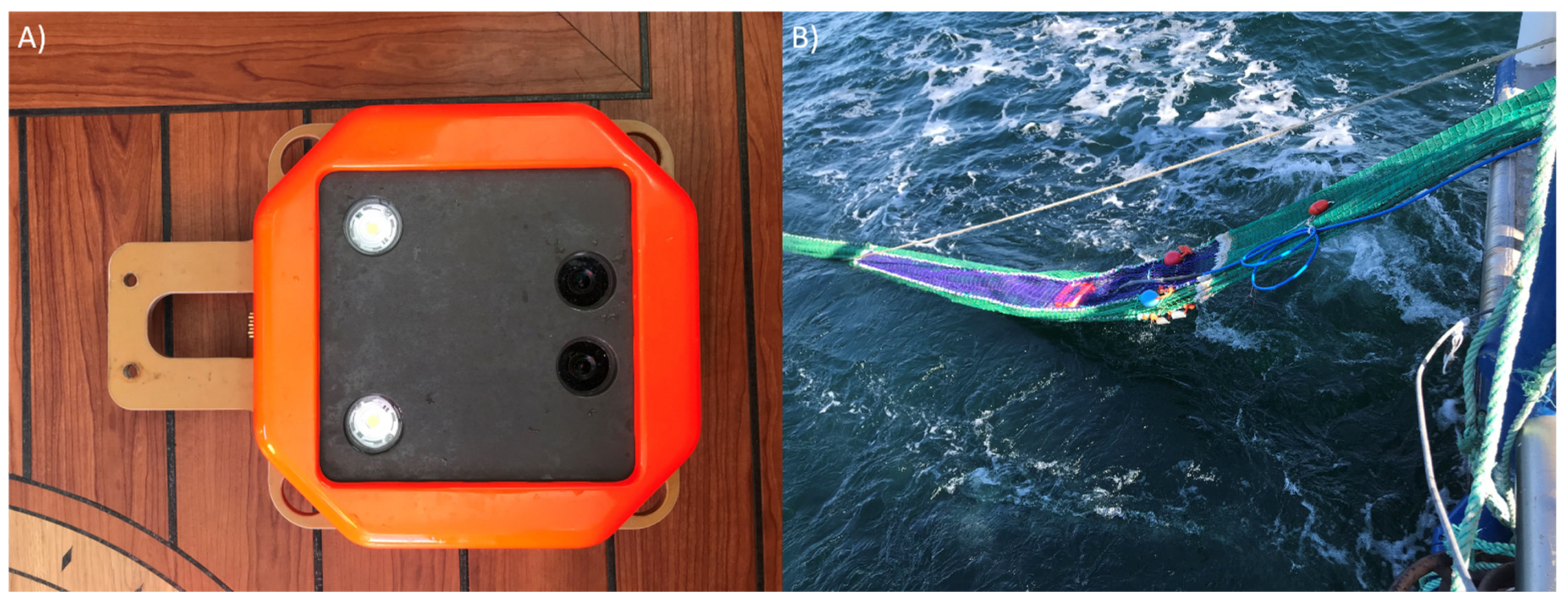
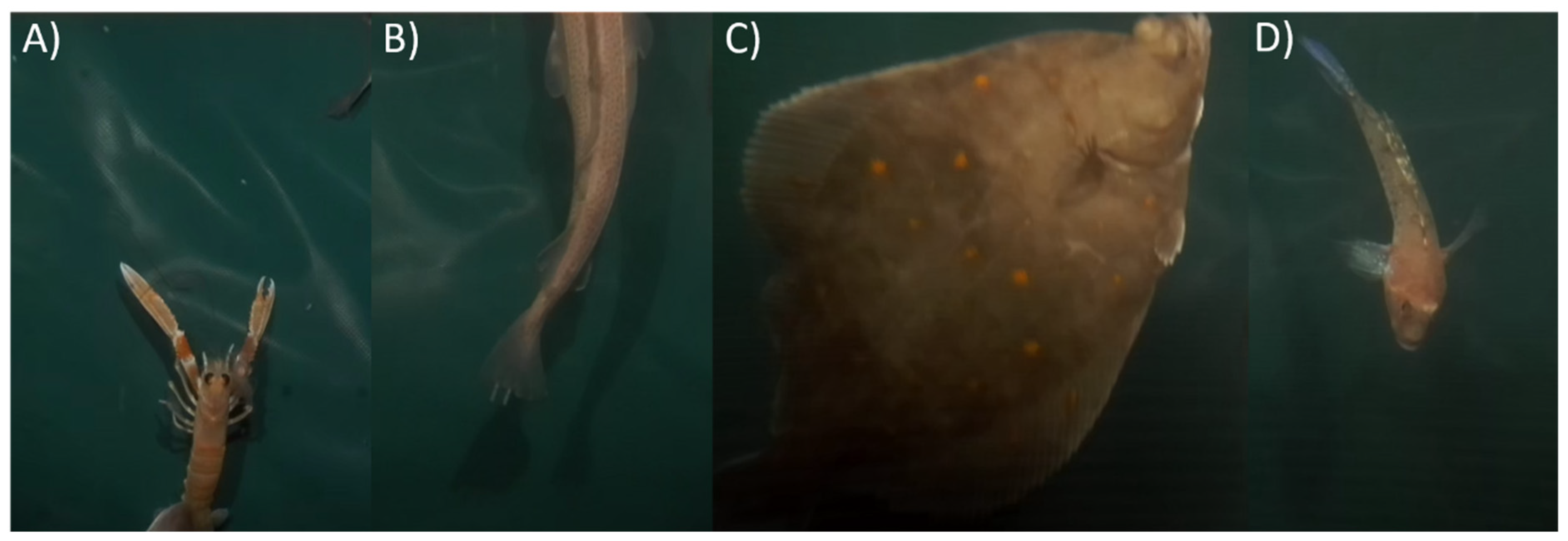
2.1. Data Preparation

To collect the video footage containing the common commercial species of the demersal trawl fishery, such as Nephrops, cod (Gadus morhua, Linnaeus, 1758) and plaice (Pleuronectes platessa, Linnaeus, 1758), we performed 19 hauls, 1.5 h duration each, in Skagerrak, onboard RV “Havfisken”. We used a low headline “Nephrops” demersal trawl with 40 mm mesh size in codend to sample all population entering the gear. To collect data of sufficient quality to enable automated detection and counting of the catch items, we used an in-trawl image acquisition system developed and described in [20]. The essential parts of that system include a camera coupled with the lights placed inside a tarpaulin cylinder, with a defined optimal color in the aft part of the trawl and a sediment-suppressing sheet attached to the ground gear of the trawl (Figure 1) [20,23]. The system ensured stable observation conditions without obscuring sediment clouds during demersal trawling and allowed us to collect high-resolution (720 p) frames to train the deep learning model. The camera settings were: 2 ms exposure, which provides the control over shutter speed; 70 gain, which is responsible for digital amplification of the signal from camera sensors; 4400 K color temperature; 60 fps frame rate.

To select the frames containing the objects of interest, the data was subsampled with the aid of a blob detector [23]. After this step, the dataset was further subsampled by a human supervisor, who selected the frames containing the target objects from the selected categories: Nephrops, round fish, flat fish and other (Figure 2). Nephrops class contained the frames depicting the target species of the demersal trawl fishery, namely Nephrops itself. Round fish class contained the frames with round fish species, such as cod, hake (Merluccius merluccius, Linnaeus, 1758) and saithe (Pollachius virens, Linnaeus, 1758). Flat fish class was composed from the frames of all flat fish species, plaice and dab (Limanda limanda, Linnaeus, 1758), for example. The other class contained the frames of different organisms such as non-commercial fish species and invertebrates, for instance, crabs.

The selected frames were manually annotated for the regions of interests and the resulting labels contained the polygons of individual objects and class ID. The prepared dataset consisted of 4385 images and was split in train and validation subsets as 88% and 12%, respectively.

2.2. Mask-RCNN Training

The architecture of Mask R-CNN was chosen to perform automated detection and classification of the objects [21]. This deep neural network is well established in the computer vision community and builds upon the previous CNN architecture (e.g., Faster R-CNN [24]. It is a two-stage detector that uses a backbone network for input image features extraction and a region proposal network to output the regions of interest and propose the bounding boxes. We used the ResNet 101-feature pyramid network (FPN) [25] backbone architecture. ResNet 101 contains 101 convolutional layers and is responsible for the bottom-up pathway, producing feature maps at different scales. The FPN then utilizes lateral connections with the ResNet and is responsible for the top-down pathway, combining the extracted features from different scales.

The network heads output the refined bounding boxes of the objects and class probabilities. In addition, as an extension of Faster R-CNN, a branch consisting of six convolutional layers provides a pixel-wise mask for the detected objects. The mask area can be used to estimate the real size of the object, which opens up a possibility to automate the catch items’ size estimation during fishing. Therefore, we chose this architecture keeping in mind the scope of future work. During training, the polygons in the labeled dataset are converted to masks of the objects. We initialized the training routine with pre-trained ImageNet weights [26]. We trained the model using Tesla V100 16 GB RAM, CUDA 11.0, cudnn v8.0.5.39, and followed the Mask RCNN Keras implementation [27].

2.3. Data Augmentation

To improve the model robustness and to avoid overfitting, we have used several image augmentation techniques during the Mask R-CNN training routine. These are instance-level transformations with Copy-Paste (CP) [28], geometric transformations, shifts in color and contrast, blur and introduction of artificial cloud-like structures [29]. To evaluate the contribution of each of the techniques, we trained a model without any augmentations used during training and considered this model a baseline for further comparisons.

CP augmentation is based on cropping instances from a source image, selecting only the pixels corresponding to the objects as indicated by their masks and pasting them on a destination image and thus substituting the original pixel values in the destination image for the ones cropped from the source. The source and destination images are subject to geometric transformations prior to CP so that the resulting image contains objects from both images with new transformations that are not present in the original dataset. The authors of CP suggest using random jitter (translation), horizontal flip and scaling. We also add vertical flip and rotation ($\theta =\left[-15°, \dots , 15°\right]$). They show that large scale variation (10%, 200%), as opposed to standard scale variation (80%, 125%), improves the performance in the COCO dataset with random weights initialization. However, we find that large scale variation generates objects with unrealistic sizes that are not expected to be found with our image acquisition setup. We find that a scale variation between 50% and 150% works best with our dataset and network configuration. We have also explored the use of several source images and performed the training with two, three and five source images. If the number of objects in the source image is more than one, then the number of the objects to be copied and pasted is defined by a random number from one to number of objects in the source image.

Data collection was undertaken using a stable image acquisition system with a tightly attached camera and an artificial light source; the illumination was not always consistent in the images due to trawl movements as well as occasional catch and sediment occlusions of the camera field of view and the light source. To make the model more robust against these changes, we used color space augmentation (referred to as “Color” augmentation) by inducing variations in hue, saturation and brightness. Specifically, the shifts were applied sequentially, starting from hue value variations (−5, 7), followed by saturation shifts (−10, 10) and, finally, the brightness changes (−20, 20). These values were derived experimentally to indicate the typical variation of color and contrast in the dataset (Figure 3).

Notwithstanding the high frame rate and the optimized ratio between exposure and gain, a degree of blur was present in the dataset. The common blur sources are the high speed of the objects’ passage through the camera field of view and the light scattering from the sediments that can partially occlude the objects. To make the model robust against these variations, we have sequentially implemented Gaussian blur with varying sigma (0.0, 3.0) and Motion blur with a ranging kernel size (5, 15). We refer to this type of tested augmentation as “Blur”.

In addition to the mentioned sources of variations in images, the occasional presence of sediment creates a set of shapes and patterns that may not be present in the training dataset and can cause false positive detections. To account for this, we explored the use of cloud augmentation (“Cloud”), which introduced random clumps of cloud-like patterns with varying sizes and colors that resembled the sediment shapes found during trawling. We set the color range by specifying the color temperature, which was set to vary from 2000 to 6000 k, corresponding to hues ranging from white to orange, approximating the real sediment colors. This type of augmentation produces an overlay, which is blended with the original image, locally changing the color of the objects lying behind the clumps and globally introducing the cloud-like patterns. Prior to “Color”, “Blur” and “Cloud” augmentations, we applied CP and geometric transformations during training.

The final model contained all the augmentation techniques applied to the images during training. The CP augmentation was applied to every training frame and the augmentations from imgaug library [29] were applied sequentially with the 40% likelihood of occurrence for each training frame. The order of augmentations applied to the image during training follows the sequence of the described augmentation techniques above.

2.4. Tracking and Counting

To track the detected objects and obtain the total automatic count of each category, we use an adaptation of the tracking algorithm SORT [22]. It relies on the Kalman filter to update the tracks’ locations and assumes a constant velocity model that corresponds to the general motion of the target species (Nephrops) during trawling [30]. However, the round fish species are able to swim together with the towed gear and are able to escape the camera field of view and re-enter it again, which typically happens when those species travel forwards towards the trawl mouth [31]. These events result in the track to disappear in the upper part of the frame; therefore, to solve this, we implement a filter in the top band of the image. In case the track disappears in the filter area, corresponding to top fifth of the image, the total count of the category does not increase.

We use the Mahalanobis distance between the tracks and detections centroids as the cost for the assignment problem, which is solved by the Hungarian algorithm [22]. We use a short probationary period, requiring only two consecutive assigned frames for a track to be considered valid. The tracks are terminated after 15 consecutive frames without being assigned any detection. Finally, we use the matching cascade algorithm proposed in [32], giving priority in the assignment problem to tracks that have been lost for fewer frames.

Our tracking problem deals with multiple classes as opposed to SORT. Often during the first few frames of an object coming into the field of view, it presents fewer distinctive features and the model is not able to assign the correct class. To address this, we allow each track to initially consider all classes before assigning a definitive one. We enable this by introducing an additional attribute to each track which consists of a vector of length equal to the number of classes. We first define the probability vector, ${\overline{p}}_i$ (Equation (1)), as the output from the softmax layer of the network consisting of the likelihoods that object i belongs to each of C classes. An important property of the softmax function is that the sum of the probabilities for ${\overline{p}}_i$ will be equal to 1.

$${\overline{p}}_i={\left[{\overline{p}}_1,\dots ,{\overline{p}}_C\right]}^T\in {\mathbb{R}}^C$$

(1)

We then define the evidence vector for track i,${\overline{v}}_i$, as the cumulative summation of probability vectors across each timestep k (Equation (2)):

$${\overline{v}}_{i,k}={\overline{v}}_{i,k-1}+{\overline{p}}_{i,k}|{\overline{v}}_{i,0}={\overline{p}}_{i,0}$$

(2)

Once the track is completed (at timestep k = K), the final confidence score and class assigned to the track are computed (Equations (3) and (4)):

$$s_i=\max \frac{{\overline{v}}_{i,K}}{K}$$

(3)

$$clas{s}_i=\arg \max {\overline{v}}_{i,K}$$

(4)

We also use the evidence vector to assist the assignment problem as well as to filter unlikely matches. In the assignment problem, an additional cost is added to the total cost, which we refer to as the $clas{s}_{cost}$ (Equation (5)):

$$clas{s}_{cost}={\displaystyle \sum }_{n=1}^C{\overline{v}}_{i,k-1,n}| n\ne \arg \max {\overline{p}}_{j,k}$$

(5)

where j is the jth object considered for assignment to track i. For a given detection-track pair, it is computed as the sum of the track’s evidence vector entries belonging to classes different than the object’s class. In the filtering stage of the matching cascade, we introduce an additional gate that forbids any assignment that has a class cost higher than a pre-established threshold.

2.5. Algorithm Evaluation

To evaluate the algorithm performance, we have selected two test videos. One with the average catch rate corresponding to typical conditions during towing (1339 s from the haul start), referred to as “Towing”, and the other with the higher occlusion rate and less stable observation conditions due to trawl movements in the end of the fishing operation (4100 s from the haul start), referred to as “Haul-back”. The first video is a typical example of the data quality and observation conditions during regular demersal trawling, whereas the second video is a stress test of the algorithm. The evaluation sample size is 27,000 and 23,100 frames corresponding to the lengths of the two test videos. The total number of test frames containing Nephrops was 2082, round fish—19,840, flat fish—3221 and other—6113.

The algorithm outputs a set of predicted tracks that we wish to evaluate against a set of ground truth tracks. The ground truth tracks are defined by the frame index where the track first appears in the video and the frame index where the track last appears in the video (start and end indices).

To compare the predicted track against the ground truth start and end indices, we construct a binary vector for each ground truth (Equation (6)),

$${\overline{a}}_i\in {\mathbb{N}}^m|{\overline{a}}_i\in \left[0,1\right]$$

(6)

where m is the number of frames between the start index of the first track and the end index of the last track present in the video and i is the ground truth index. We set the elements of ${\overline{a}}_i$ to be 1 between the start and end indices of the corresponding ground truth. The rest are set to 0. We construct a similar vector for the predictions, ${\overline{b}}_j\in {\mathbb{Z}}^n|{\overline{b}}_j\in \left[0,1\right]$, where n is the number of predicted tracks.

We then calculate the Intersection over Union (IoU) for each pair of ${\overline{a}}_i$ and ${\overline{b}}_j$ (Equation (7)):

$$Io{U}_{ij}=\frac{{\overline{a}}_i\cap {\overline{b}}_j}{{\overline{a}}_i\cup {\overline{b}}_j}$$

(7)

We are interested in solving the assignments between ground truths G and predictions P via maximizing the summed IoU, so we formulate the general assignment problem as a linear program (Equations (8)–(13)):

$$\mathrm{maximise}{\displaystyle \sum }_{\left(i,j\right)G\times P}{J}_{i,j}{x}_{i,j}$$

(8)

$$\mathrm{s}.\mathrm{t}.{\displaystyle \sum }_{j\in P}{x}_{ij}=1 \mathrm{for} i\in G$$

(9)

$${\displaystyle \sum }_{i\in G}{x}_{ij}=1\mathrm{for} j\in P$$

(10)

$$0\le x_{ij}\le 1 \mathrm{for} i,j\in G,P$$

(11)

$$x_{ij}\in \mathbb{Z} \mathrm{for} i,j\in G,P$$

(12)

$$J_{ij}=\{\begin{array}{c}-1 \mathrm{if} Io{U}_{ij}\le \kappa \\ Io{U}_{ij}\mathrm{if}>\kappa \end{array} ,$$

(13)

where the final definition of IoU enforces a penalty for assigning tracks that have an IoU that is less than or equal to some threshold value $\kappa$ ($\kappa =0).$ The solution to Equation (8) yields optimal matches between ground truth and predictions. The solver implementation used the GNU Linear Programming Kit (GLPK) simplex method [33]. (The matched ground truth tracks and the predicted tracks are treated as True Positives (TP), unmatched ground truth tracks correspond to False Negatives (FN) and the unmatched predicted tracks corresponds to False Positives (FP)). The number of TP, FN and FP were used to calculate Precision, Recall and the F-score of the algorithm.

2.6. Automated and Manual Catch Comparison

The two best performing algorithms were used to predict the total count of the catch items in the two selected test videos to diagnose automated count progress in relation to video frames. We then applied both algorithms to the other nine videos containing the catch monitoring during the whole fishing operation (haul). Predicted count for the whole haul was then compared with the manual count of the catch captured by the in-trawl image acquisition system and the actual catch count performed onboard the vessel. We have calculated an absolute error ($E$) (Equation (14)) of the predicted catch count to evaluate the algorithm performance in catch description of the entire haul.

$$E=x_j-x_i,$$

(14)

where $x_i$ denotes the ground truth count and $x_j$ corresponds to the predicted by the algorithm count per class.

All Nephrops were identified and counted onboard the vessel. Only the commercial species were counted onboard among the other three classes. Thus, cod and hake were counted onboard in the round fish category; plaice, lemon sole (Microstomus kitt, Walbaum, 1792) and witch flounder (Glyptocephalus cynoglossus, Linnaeus, 1758) were counted corresponding to the flat fish class; and squid (Loligo vulgaris, Lamarck, 1798) was counted for the other class.

3. Results

3.1. Training

The selected values for the learning rate varied from 0.0003 to 0.0005 (

Table 1. Tuned hyperparameter values for each of the augmentation techniques derived from experiments. CP—Copy-Paste augmentation.

	Hyperparameters	Learning Rate	Number of Epochs	Steps per Epoch	Batch Size	Source Images for CP
Types of Augmentation
Baseline (none)		0.0005	60	1000	2	3
CP and Geometric transformations		0.0005	76		2
Blur		0.0005	80		1
Color		0.0003	100		2
Cloud		0.0004	84		2
All augmentations		0.0005	76		2

). The specific values were chosen to prevent exploding gradient resulting in backpropagation failure. The ‘ReduceOnPlateau’ Keras function has been implemented to drop the learning rate by half if the validation loss has stopped decreasing during 12 epochs. The lowest bound for the learning rate was set to 0.0001. The small value for the learning rate required more iterations of training; therefore, the number of epochs for the best performing models were above 60 epochs with a maximum of 100 epochs. We have explored the use of one and two images per batch and, in general, the model performance was observed to be higher with the use of two images per batch, excepting the model trained with the blur augmentation. We have also experimented with the number of source images providing the instances to be pasted to the destination training image. The number of source images varied from two to five, which provided similar model performance; however, the use of three source images provided the highest scores.

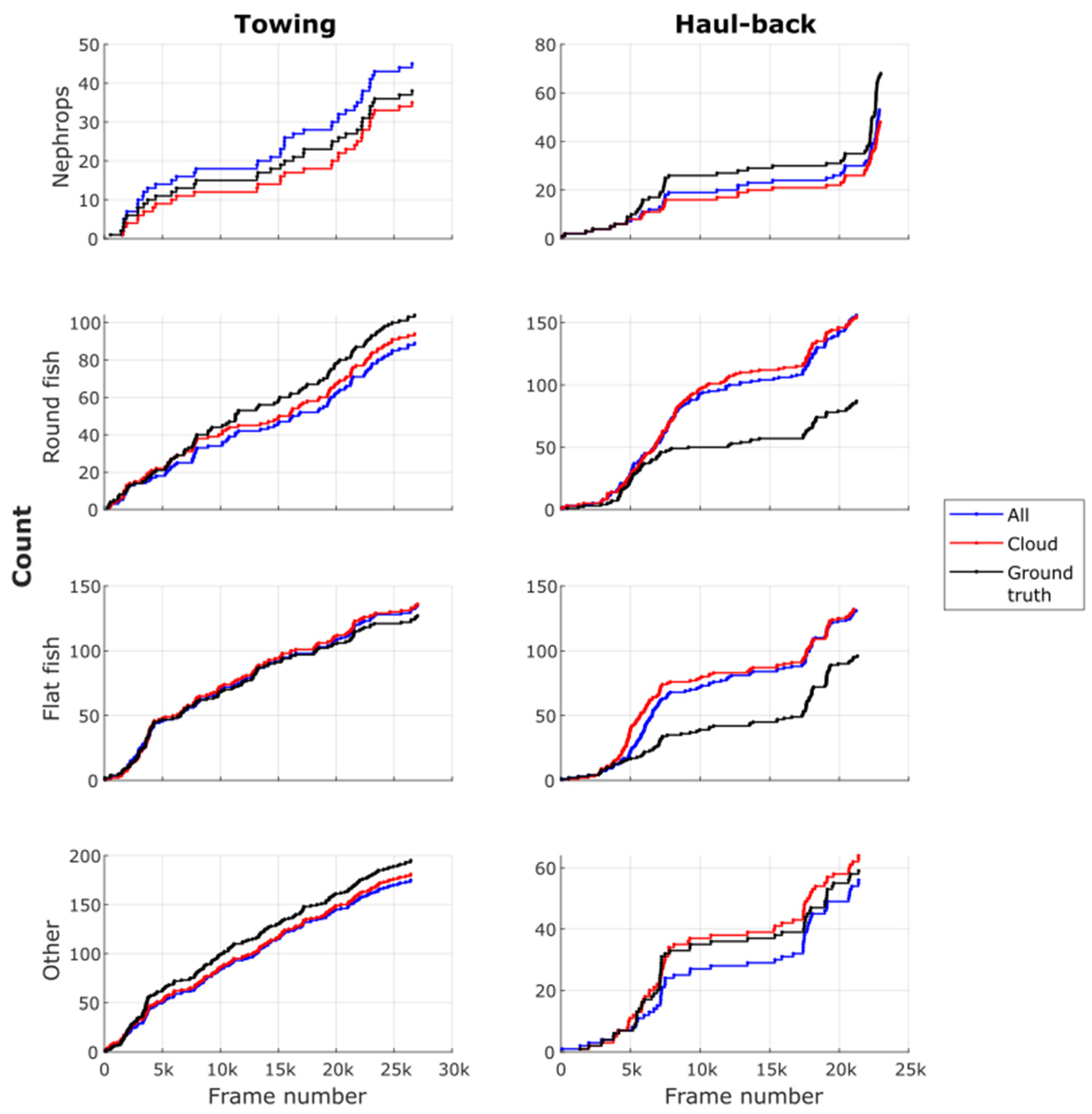
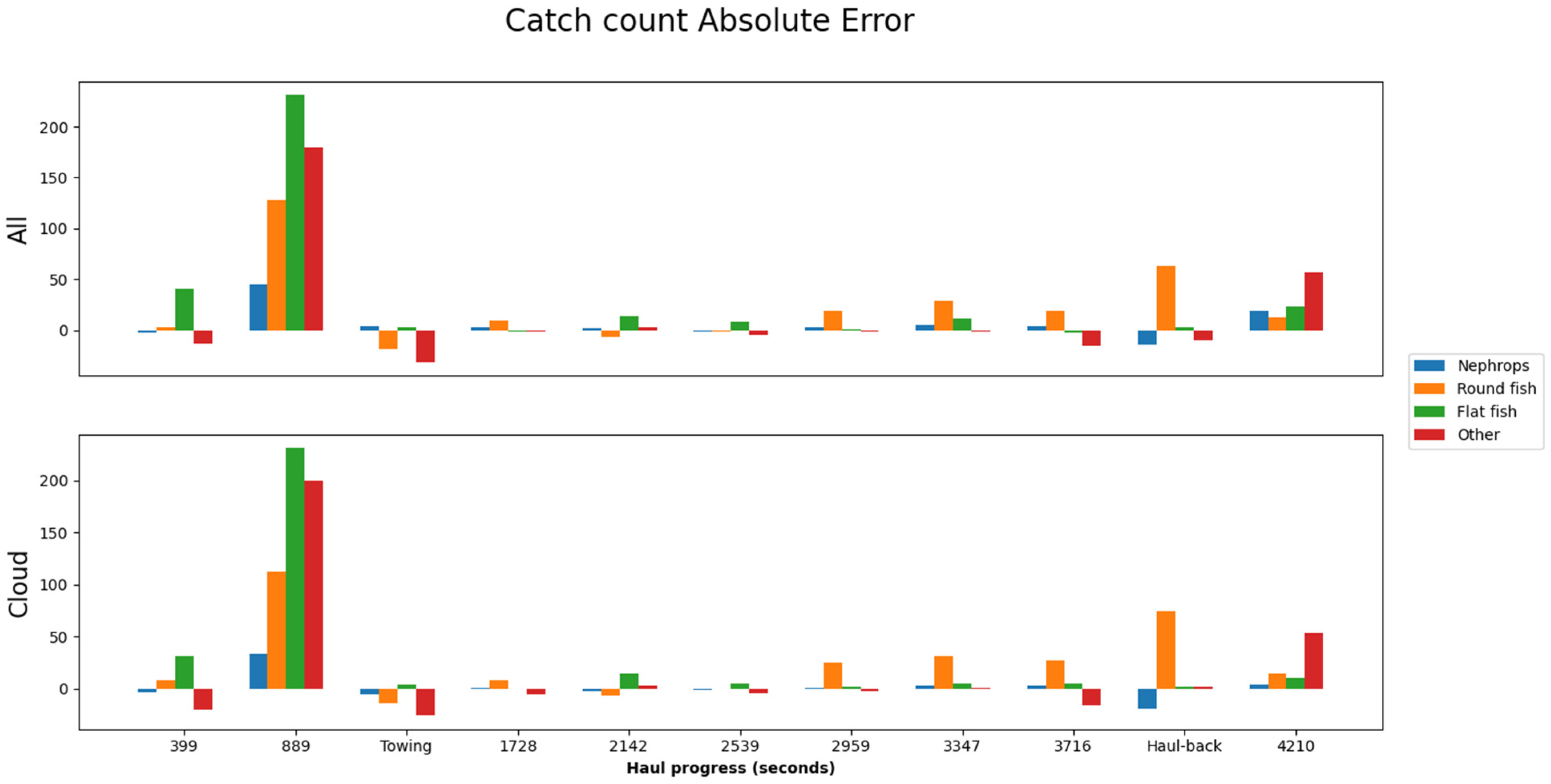
3.2. Evaluation

As we are interested in the total catch automated description, we have averaged the resulting F-scores among the four categories and used it as a major indicator of the algorithms’ performance (Figure 4). The first pattern that can be captured from the first glance at Figure 4 is the algorithms’ difference in performance while applied to the two test videos. Overall, the algorithms’ F-score applied to the “Haul-back” video case showed lower values compared to the “Towing” video. In case of the baseline model, the F-score was 15% lower while tested on the “Haul-back” video compared to the trawling scenario.

Among all the studied detectors, testing of the algorithm with the baseline model expectedly showed the lowest F-scores in both video test cases. The highest F-score of 0.79 was reached with the algorithm utilizing Mask R-CNN trained with all augmentations applied to the “Towing” case video. In the case of the “Haul-back” video case, the algorithm with Mask R-CNN trained with CP, geometric transformations and cloud augmentation showed a slightly higher F-score than that of the algorithm with the detection based on the model trained with all augmentations.

The explicit table (

Table A1. Precision, Recall and F-score metrics calculated for each of the models trained with the four test augmentation techniques. The performance was evaluated on the video with the average catch rate and lower presence of occlusions (“Towing”) and on a stress test video with less stable observation conditions and higher occlusion rate (“Haul-back”). The values are listed in columns for the four classes: Nephrops, round fish, flat fish, other.

Type of Augmentation	Precision		Recall		F-Score
	Towing	Haul-Back	Towing	Haul-Back	Towing	Haul-Back
Baseline (none)	0.694	0.650	0.829	0.743	0.756	0.693
	0.504	0.409	0.546	0.785	0.524	0.538
	0.534	0.437	0.886	0.909	0.667	0.590
	0.693	0.381	0.884	0.750	0.777	0.506
Average	0.606	0.469	0.786	0.797	0.681	0.582
Copy-Paste and Geometric transformations	0.661	0.800	0.902	0.800	0.763	0.800
	0.642	0.480	0.731	0.849	0.684	0.613
	0.795	0.588	0.879	0.879	0.835	0.704
	0.821	0.423	0.865	0.683	0.842	0.522
Average	0.730	0.573	0.844	0.803	0.781	0.660
Blur	0.745	0.867	0.854	0.743	0.796	0.800
	0.677	0.461	0.602	0.791	0.637	0.582
	0.663	0.515	0.864	0.869	0.750	0.647
	0.814	0.458	0.783	0.633	0.798	0.531
Average	0.725	0.575	0.776	0.759	0.745	0.640
Color	0.761	0.813	0.854	0.743	0.805	0.776
	0.735	0.500	0.565	0.802	0.639	0.616
	0.728	0.558	0.932	0.919	0.817	0.695
	0.785	0.386	0.865	0.733	0.823	0.506
Average	0.752	0.564	0.804	0.799	0.771	0.648
Cloud	0.773	0.844	0.829	0.771	0.800	0.806
	0.652	0.482	0.676	0.860	0.664	0.618
	0.788	0.506	0.902	0.838	0.841	0.631
	0.845	0.551	0.845	0.717	0.845	0.623
Average	0.765	0.596	0.813	0.797	0.788	0.670
All augmentations	0.696	0.763	0.951	0.829	0.804	0.795
	0.658	0.482	0.694	0.837	0.676	0.612
	0.805	0.481	0.909	0.889	0.854	0.624
	0.842	0.597	0.826	0.667	0.834	0.630
Average	0.751	0.581	0.845	0.806	0.792	0.665

) containing the values of the calculated Precision, Recall and F-score for all four categories in the two case videos are presented in Appendix A. The detection examples obtained with using the Mask R-CNN trained with all augmentations as a detector on the “Towing” and “Haul-back” video frames are presented in Figure 5.

3.3. Comparison of Automated and Manual Catch Descriptions

Automated count estimated per frame of the test videos was closer to the ground truth count in the case of the “Towing” test video (Figure 6), supporting the algorithms’ higher F-scores (Figure 4). During the “Haul-back”, the automated count of Nephrops had a tendency towards underestimation by both algorithms, whereas in the case of round fish and flat fish classes an opposite trend of overestimation was observed. In the case of the other class, the algorithm based on training with “Cloud” augmentations approximated the real count better compared to the algorithm output with all test augmentations implemented during training.

Manual catch count onboard deviates from the ground truth count in the videos due to the catch items avoiding the camera field of view and due to the variations in class assignment criteria (

Table 2. Automated (predicted) and manual catch count results per class.

	Class	Nephrops	Round Fish	Flat Fish	Other
Types of Augmentation
Manual catch count (onboard)		323	464	556	9
Manual catch count (videos)		235	530	755	897
Baseline (none)		302	869	1439	1383
CP and Geometric transformations		282	819	1078	1114
Blur		272	889	1179	1027
Color		262	691	1174	1256
Cloud		249	808	1064	1082
All augmentations		302	785	1084	1058

). All captured Nephrops, both in the resulting catch and captured by an in-trawl image acquisition system, were counted. In case of the round fish and flat fish classes, only the commercial species were counted onboard. The criteria of assigning catch items to round fish and flat fish classes for the automated detection and count purpose was based on the object aspect ratio assumption. Thus, in addition to the commercial species counted onboard, a number of non-commercial species contribute to the manual count in the videos. The reason for the mismatch in the manual count of the other class onboard and in the videos is similar. Only one species is considered commercial in this class and hence counted onboard.

We can conclude that 73% of Nephrops are being recorded by an in-trawl image acquisition system. The algorithm based on Mask R-CNN training with “Cloud” augmentations applied outputs the closest to the manual count. An average F-score of this algorithm is 0.73, estimated for the two test videos (Table A1). All of the algorithms tend to overestimate the count of the other three classes. Figure 7 reveals the time interval of the fishing operation that corresponds to the largest automated count bias occurrence.

The largest absolute error of the predicted automated count output by the two best performing algorithms was observed in the video depicting the initialization of the catch process. This time stamp corresponds to the phase of the fishing operation when the trawl gets in contact with the seabed which causes increased sediment resuspension, the presence of which contributes to the count bias towards false positive detections. During towing, the absolute error in the automated count produced by both algorithms remains low. The video recordings of the catch monitoring during the entire trawling are available as the data supporting the reported results [34].

4. Discussion

In this study, we have described the automated video processing solution for catch description during commercial demersal trawling. The algorithm is tuned for a dataset collected in the Nephrops-directed mixed species fishery, which is obtained with the aid of the in-trawl observation section enabling sediment-free video footage during demersal trawling. The use of augmentations during training boosted the algorithm performance for both the towing and haul-back phase of the trawling operation. Based on the absolute error estimation of the automated count, we can conclude that the algorithm’s performance is challenged in the demersal trawling initialization phase. However, the error in the automated count remained low during towing, corresponding to the core of the demersal trawling. These results indicate readiness of the proposed solution for at-sea application. Considering today’s conditions for the demersal trawling practice, which is today more or less a blind process, the system has the potential to transform the traditional demersal trawl fishery to a more informed, targeted and efficient process.

4.1. Towards Precision Fishing

The concept of precision fishing implies advanced analytics for big data collected by ubiquitous perception devices [35]. The resulting analysis of the videos collected on-board can provide detailed catch statistics. Today, such on-board monitoring systems are primarily used by managers and scientists to establish and update the regulations in a reactive manner. The demonstrated approach presents the possibility for fishers to utilize this information directly during the fishing process, which is an assertive management tool rather than reactive. The system application on a commercial scale offers a win-win solution for both fishers and managers. Using the obtained information regarding the catch composition and amount, fishers can react immediately to the presence of bycatch and thereby make their process more targeted and efficient, which will align ecological and economic sustainability.

The system is developed for commercial trawl fisheries, using the Nephrops-directed trawl fishery as a case study. The amount of bycatch in the mixed demersal trawl fishery targeting Nephrops is higher compared to the mixed fishery targeting fish species [2]. Thus, the proposed solution is expected to have a higher impact while applied to this fishery. Nephrops-directed fisheries operate with low headline demersal trawls [5] where the implementation of monitoring devices is challenged by the smaller gear dimensions and the proximity to the seabed. We have demonstrated that the developed in-trawl observation system and the automated catch description approach is effective in this fishery. Demersal trawl fisheries that are targeting other species also experience similar challenges as the Nephrops fishery [1] so we expect that the proposed optical monitoring tool can be adapted for the majority of the demersal trawl fisheries, following further acquisition of species-specific data and labelling. With an increasing demand for seafood, the introduction of the novel technology that can improve extraction patterns in the commercial fisheries is crucial for sustainable use of limited natural resources [35].

4.2. Algorithm Performance

The tested algorithms performed worse on the “Haul-back” video compared to “Towing” video (Figure 4; Table A1). This observation is expected as changing hydrodynamic conditions alter the background panel position, which may contribute to FP detections of the background as an object due to reflection of light and irregular curvatures. Besides, some fish species hold in front of the observation section for longer periods of time during the towing phase and first fall through haul-back is initiated, causing a heavy increase in occlusion due to crowding. However, such conditions are present when the trawl is hauled back; thus, at that point, the decision to terminate the fishing operation has already been made. Our findings indicate that the algorithms are suitable for serving as an automated processing tool of the video stream and work as a decision support tool for the fishers to avoid manual analysis of the videos. The system efficiency as a decision support tool relies on the algorithm performance accuracy, provided it is high. In this study, we have demonstrated the maximum of 0.79 F-score via improving the accuracy of detection (Appendix A and Appendix B) and by extending the SORT algorithm with implementing evidence vector for more accurate class-to-track assignment as well as cascade matching to reduce the erroneous detection to track assignment between overlapping objects. The duplicate counts of the objects escaping from the top band of the frame were accounted for by introducing a filter in the top fifth rows of the frame.

Mask RCNN showed to be an efficient tool in the related studies of the catch registration on the conveyer belt as well as the in-trawl catch monitoring in pelagic fishery [13,14,15]. To our knowledge, we present the first solution for automated catch description for the commercial demersal trawl fishery. It is made possible by using a systematic approach for ensuring the data quality during towing and fine-tuning the algorithm to the collected data. We foresee the necessity in additional fine-tuning of the algorithm to be effectively used in different conditions. Under the system implementation by the end users, we expect the detection accuracy improvement as more data will be collected and used to update the existing one [36].

4.3. Algorithm Real-World Application

To implement an effective decision support tool for fishers, the automated data processing needs to be close to real time. The proposed algorithm needs approximately 6000 s to process the “Towing” and “Haul-back” videos, which are of 450 s and 385 s, respectively. Our proposed solution can be optimized to leverage the inference speed of Mask R-CNN via NVIDIA TensorRT™. Another option is to consider another model architecture, such as single-stage detectors, which do not provide the pixel-wise mask information, essential for precise size estimation, but are much faster. At the data acquisition level, the input video stream can be subsampled to process every $n_{th}$ frame of the input video, and the SORT component of the algorithm must be tuned for the resulting reduction in update rate.

Automated and manual catch count comparison indicated the difference in absolute error peaking in trawling initialization phase (Figure 7). This phase corresponds to 11% of the total fishing operation duration. It is a routine procedure, therefore, the time required to initialize trawling will be similar among the operations. Thus, this percentage will be reduced with longer trawling and hence cause a lower impact on the resulting count accuracy. Additionally, during this phase, the trawl is not fully operational as, during this time interval, the trawl geometry is unstable as the gear is in the process of settling at the seabed, which may result in the reduced number of catch items entering the gear.

4.4. Prospective Applications

The application of the Mask R-CNN architecture in combination with the use of stereo camera also allows obtaining automated size estimations of the catch. The automated length estimations of fish with aid of Mask R-CNN showed to be efficient and the approaches are demonstrated by extrapolating the estimated fish head length to the total length via a modelled ratio [37]. Another study by Yu et al. [38] demonstrates the measurements of the body and caudal peduncle lengths and widths, eye and pupil diameters of the target fish species. These studies suggest that the total fish size estimation can be derived from the sizes of the specific features of animals. Considering Nephrops, the size of which are initially estimated from the carapace length [39] and the fact that most of the individuals have the carapace visible in the camera field of view, there is an opportunity to register the size measurements automatically as well.

5. Conclusions

The proposed solution is a part of a catch monitoring tool developed for the commercial demersal trawl fishery and has the potential to transform these fisheries from a blind to an informed process where the fisher can automatically obtain the composition and number of species in the catch. The algorithm showed the high performance during the towing conditions and, therefore, can be applied for automated data processing and act as a decision support tool for fishers, provided the adjustments towards near real-time performance. The future work includes embedding the algorithm on a portable hardware for practical use and exploring the possibilities for automated catch measurements.

References

- Kennelly, S.J.; Broadhurst, M.K. A review of bycatch reduction in demersal fish trawls. Rev. Fish Biol. Fish. 2021, 31, 289–318. [Google Scholar] [CrossRef]
- Rihan, D. Research for PECH Committee—Landing Obligation and Choke Species in Multispecies and Mixed Fisheries—The North Western Waters; Policy Department for Structural and Cohesion Policies, European Parliament: Brusseles, Brusseles, 2018. [Google Scholar]
- EU Council Regulation. Fixing for 2019 the Fishing Opportunities for Certain Fish Stocks and Groups of Fish Stocks, Applicable in Union Waters and for Union Fishing Vessels in Certain Non-Union Waters. In Official Journal of the European Union; European Union: Maastricht, The Netherlands, 2019. [Google Scholar]
- Pérez Roda, M.A.; Gilman, E.; Huntington, T.; Kennelly, S.J.; Suuronen, P.; Chaloupka, M.; Medley, P. A Third Assessment of Global Marine Fisheries Discards; FAO Fisheries and Aquaculture Technical Paper No. 633; FAO: Rome, Italy, 2019; p. 78. [Google Scholar]
- Graham, N.; Ferro, R.S.T. The Nephrops Fisheries of the Northeast Atlantic and Mediterranean: A Review and Assessment of Fishing Gear Design; ICES Cooperative Research Report No. 270; International Council for the Exploration of the Sea: Copenhagen, Denmark, 2004. [Google Scholar]
- DeCelles, G.R.; Keiley, E.F.; Lowery, T.M.; Calabrese, N.M.; Stokesbury, K.D.E. Development of a Video Trawl Survey System for New England Groundfish. Trans. Am. Fish. Soc. 2017, 146, 462–477. [Google Scholar] [CrossRef]
- Rosen, S.; Holst, J.C. DeepVision in-trawl imaging: Sampling the water column in four dimensions. Fish. Res. 2013, 148, 64–73. [Google Scholar] [CrossRef]
- Mallet, D.; Pelletier, D. Underwater video techniques for observing coastal marine biodiversity: A review of sixty years of publications (1952–2012). Fish. Res. 2014, 154, 44–62. [Google Scholar] [CrossRef]
- Underwood, M.J.; Rosen, S.; Engås, A.; Eriksen, E. Deep Vision: An In-Trawl Stereo Camera Makes a Step Forward in Monitoring the Pelagic Community. PLoS ONE 2014, 9, e112304. [Google Scholar] [CrossRef] [PubMed] [Green Version]
- Williams, K.; Lauffenburger, N.; Chuang, M.-C.; Hwang, J.-N.; Towler, R. Automated measurements of fish within a trawl using stereo images from a Camera-Trawl device (CamTrawl). Methods Oceanogr. 2016, 17, 138–152. [Google Scholar] [CrossRef]
- Allken, V.; Handegard, N.O.; Rosen, S.; Schreyeck, T.; Mahiout, T.; Malde, K. Fish species identification using a convolutional neural network trained on synthetic data. ICES J. Mar. Sci. 2018, 76, 342–349. [Google Scholar] [CrossRef]
- Christensen, J.H.; Mogensen, L.V.; Galeazzi, R.; Andersen, J.C. Detection, Localization and Classification of Fish and Fish Species in Poor Conditions using Convolutional Neural Networks. In Proceedings of the 2018 IEEE/OES Autonomous Underwater Vehicle Workshop (AUV), IEEE, Porto, Portugal, 6–9 November 2018; pp. 1–6. [Google Scholar]
- Tseng, C.-H.; Kuo, Y.-F. Detecting and counting harvested fish and identifying fish types in electronic monitoring system videos using deep convolutional neural networks. ICES J. Mar. Sci. 2020, 77, 1367–1378. [Google Scholar] [CrossRef]
- French, G.; Mackiewicz, M.; Fisher, M.; Holah, H.; Kilburn, R.; Campbell, N.; Needle, C. Deep neural networks for analysis of fisheries surveillance video and automated monitoring of fish discards. ICES J. Mar. Sci. 2019, 77, 1340–1353. [Google Scholar] [CrossRef]
- Garcia, R.; Prados, R.; Quintana, J.; Tempelaar, A.; Gracias, N.; Rosen, S.; Vågstøl, H.; Løvall, K. Automatic segmentation of fish using deep learning with application to fish size measurement. ICES J. Mar. Sci. 2019, 77, 1354–1366. [Google Scholar] [CrossRef]
- O’Mahony, N.; Campbell, S.; Carvalho, A.; Harapanahalli, S.; Hernandez, G.V.; Krpalkova, L.; Riordan, D.; Walsh, J. Deep Learning vs. Traditional Computer Vision. In Advances in Computer Vision; Springer International Publishing: Cham, Switzerland, 2019; pp. 128–144. [Google Scholar] [CrossRef] [Green Version]
- Mariani, P.; Quincoces, I.; Haugholt, K.H.; Chardard, Y.; Visser, A.W.; Yates, C.; Piccinno, G.; Reali, G.; Risholm, P.; Thielemann, J.T. Range-Gated Imaging System for Underwater Monitoring in Ocean Environment. Sustainability 2018, 11, 162. [Google Scholar] [CrossRef] [Green Version]
- Thomsen, B. Selective Flatfish Trawling. ICES Mar. Sci. Symp. 1993, 196, 161–164. [Google Scholar]
- Krag, L.A.; Madsen, N.; Karlsen, J.D. A study of fish behaviour in the extension of a demersal trawl using a multi-compartment separator frame and SIT camera system. Fish. Res. 2009, 98, 62–66. [Google Scholar] [CrossRef]
- Sokolova, M.; O’Neill, F.G.; Savina, E.; Krag, L.A. Test and Development of a Sediment Suppressing System for Catch Monitoring in Demersal Trawls; Submitted to Fisheries Research; National Institute of Aquatic Resources, Technical University of Denmark: Hirtshals, Denmark, 2021. [Google Scholar]
- He, K.; Gkioxari, G.; Dollár, P.; Girshick, R. Mask R-CNN. arXiv 2017, arXiv:1703.06870. [Google Scholar]
- Bewley, A.; Ge, Z.; Ott, L.; Ramos, F.; Upcroft, B. Simple online and realtime tracking. In Proceedings of the 2016 IEEE International Conference on Image Processing (ICIP), Phoenix, AZ, USA, 25–28 September 2016; pp. 3464–3468. [Google Scholar]
- Sokolova, M.; Thompson, F.; Mariani, P.; Krag, L.A. Towards sustainable demersal fisheries: NepCon image acquisition system for automatic Nephrops norvegicus detection. PLoS ONE 2021, 16, e0252824. [Google Scholar] [CrossRef]
- Ren, S.; He, K.; Girshick, R.; Sun, J. Faster R-CNN: Towards Real-Time Object Detection with Region Proposal Networks. IEEE Trans. Pattern Anal. Mach. Intell. 2017, 39, 1137–1149. [Google Scholar] [CrossRef] [PubMed] [Green Version]
- Lin, T.Y.; Dollár, P.; Girshick, R.; He, K.; Hariharan, B.; Belongie, S. Feature pyramid networks for object detection. In Proceedings of the IEEE Conference on Computer Vision and Pattern Recognition, Honolulu, HI, USA, 21–26 July 2017; pp. 2117–2125. [Google Scholar] [CrossRef] [Green Version]
- Deng, J.; Dong, W.; Socher, R.; Li, L.J.; Li, K.; Li, F.F. Imagenet: A Large-Scale Hierarchical Image Database. In Proceedings of the 2009 IEEE Conference on Computer Vision and Pattern Recognition, Miami, FL, USA, 20–25 June 2009; pp. 248–255. [Google Scholar]
- Abdulla, W. Mask R-CNN for Object Detection and Instance Segmentation on Keras and TensorFlow. 2017. Available online: https://github.com/matterport/Mask_RCNN (accessed on 8 February 2021).
- Ghiasi, G.; Cui, Y.; Srinivas, A.; Qian, R.; Lin, T.-Y.; Cubuk, E.D.; Le, Q.V.; Zoph, B. Simple Copy-Paste is a Strong Data Augmentation Method for Instance Segmentation. In Proceedings of the 2021 IEEE/CVF Conference on Computer Vision and Pattern Recognition (CVPR), Virtual, 19–25 June 2021; pp. 2917–2927. [Google Scholar]
- Jung, A. Imgaug Documentation, Release 0.4.0. 2020. Available online: https://imgaug.readthedocs.io/en/latest/ (accessed on 28 July 2021).
- Catchpole, T.L.; Revill, A.S. Gear technology in Nephrops trawl fisheries. Rev. Fish Biol. Fish. 2008, 18, 17–31. [Google Scholar] [CrossRef]
- Winger, P.D.; Eayrs, S.; Glass, C.W. Fish Behavior near Bottom Trawls. In Behavior of Marine Fishes: Capture Processes and Conservation Challenges; He, P., Ed.; Wiley-Blackwell: Ames, IA, USA, 2010; pp. 67–95. [Google Scholar]
- Wojke, N.; Bewley, A.; Paulus, D. Simple online and realtime tracking with a deep association metric. In Proceedings of the 2017 IEEE International Conference on Image Processing (ICIP), Beijing, China, 17–20 September 2017; pp. 3645–3649. [Google Scholar]
- Makhorin, A. GNU Linear Programming Kit Reference Manual for GLPK Version 4.45. 2010. Available online: https://www.gnu.org/software/glpk/ (accessed on 20 August 2021).
- Sokolova, M.; Alepuz, A.M.; Thompson, F.; Mariani, P.; Galeazzi, R.; Krag, L.A. Catch Monitoring via a Novel In-Trawl Image Acquisition System during Demersal Trawling. Data Repository. 2021. Available online: https://doi.org/10.11583/DTU.16940173.v2 (accessed on 5 November 2021).
- Christiani, P.; Claes, J.; Sandnes, E.; Stevens, A. Precision Fisheries: Navigating a Sea of Troubles with Advanced Analytics. 2019. Available online: https://www.mckinsey.com/industries/agriculture/our-insights/precision-fisheries-navigating-a-sea-of-troubles-with-advanced-analytics (accessed on 15 September 2021).
- Shorten, C.; Khoshgoftaar, T.M. A survey on Image Data Augmentation for Deep Learning. J. Big Data 2019, 6, 60. [Google Scholar] [CrossRef]
- Álvarez-Ellacuría, A.; Palmer, M.; Catalán, I.A.; Lisani, J.-L. Image-based, unsupervised estimation of fish size from commercial landings using deep learning. ICES J. Mar. Sci. 2020, 77, 1330–1339. [Google Scholar] [CrossRef]
- Yu, C.; Fan, X.; Hu, Z.; Xia, X.; Zhao, Y.; Li, R.; Bai, Y. Segmentation and measurement scheme for fish morphological features based on Mask R-CNN. Inf. Process. Agric. 2020, 7, 523–534. [Google Scholar] [CrossRef]
- Graham, N.; Jones, E.; Reid, D. Review of technological advances for the study of fish behaviour in relation to demersal fishing trawls. ICES J. Mar. Sci. 2004, 61, 1036–1043. [Google Scholar] [CrossRef] [Green Version]
- Frid-Adar, M.; Diamant, I.; Klang, E.; Amitai, M.; Goldberger, J.; Greenspan, H. GAN-based synthetic medical image augmentation for increased CNN performance in liver lesion classification. Neurocomputing 2018, 321, 321–331. [Google Scholar] [CrossRef] [Green Version]
- Taylor, L.; Nitschke, G. Improving Deep Learning Using Generic Data Augmentation. In Proceedings of the 2018 IEEE Symposium Series on Computational Intelligence (SSCI), Bangalore, India, 18–21 November 2018. [Google Scholar]