Article

Model Reduction Applied to Empirical Models for Biomass Gasification in Downdraft Gasifiers

by
Michael Binns
* and
Hafiz Muhammad Uzair Ayub
Department of Chemical and Biochemical Engineering, Dongguk University-Seoul, 30 Pildong-ro 1-gil, Jung-gu, Seoul 04620, Korea
*
Author to whom correspondence should be addressed.
Sustainability 2021, 13(21), 12191; https://doi.org/10.3390/su132112191
Submission received: 4 October 2021 / Revised: 28 October 2021 / Accepted: 3 November 2021 / Published: 4 November 2021

Abstract

:
Various modeling approaches have been suggested for the modeling and simulation of gasification processes. These models allow for the prediction of gasifier performance at different conditions and using different feedstocks from which the system parameters can be optimized to design efficient gasifiers. Complex models require significant time and effort to develop, and they might only be accurate for use with a specific catalyst. Hence, various simpler models have also been developed, including thermodynamic equilibrium models and empirical models, which can be developed and solved more quickly, allowing such models to be used for optimization. In this study, linear and quadratic expressions in terms of the gasifier input value parameters are developed based on linear regression. To identify significant parameters and reduce the complexity of these expressions, a LASSO (least absolute shrinkage and selection operator) shrinkage method is applied together with cross validation. In this way, the significant parameters are revealed and simple models with reasonable accuracy are obtained.

1. Introduction

The gasification of biomass allows for the production of syngas, consisting of hydrogen and carbon monoxide, which can be used as fuel or converted to other products. This is a renewable source of energy which can take various types of biomass, including wood, straw, and various crop residues, such as shells or husks etc.
To aid the design of gasification systems, modeling can be used to avoid the cost of expensive experiments for the prediction of output composition using different feedstocks and under various operating conditions [1]. The review of Patra and Sheth mentions several categories of model biomass gasifiers including more complex models based on kinetic rate expressions or computational fluid dynamics, in addition to relatively simpler models based on thermodynamic equilibrium assumptions and empirical models based on artificial neural networks [1]. In addition, they mention the possibility of modeling inside a process simulator such as Aspen Plus, which may include kinetic or equilibrium models, for example, inside the process units or associated subroutines [1]. For example, Safarian et al. simulated a gasification process in Aspen Plus using a Gibbs reactor to calculate the equilibrium point minimizing the Gibbs free energy [2]. Marcantonio et al. also modeled gasification using a Gibbs reactor inside Aspen Plus, which they compared against a more accurate kinetic model simulated in MATLAB [3].
To avoid the complexities associated with kinetic and CFD (computational fluid dynamics) models, a large number of studies have focused on equilibrium models, artificial neural networks, and other empirical or semi-empirical models which allow for the fast simulation, sensitivity analysis, and optimization of gasification systems. However, equilibrium models are known to have some inaccuracy because the real gasifier does not necessarily reach equilibrium and can lead to an overestimation of the hydrogen and carbon monoxide content of producer gas and an underestimation of methane content [4]. To address this inaccuracy, a number of studies have proposed adding correction factors or correlations to the equilibrium models to make the results closer to reality as detailed in the review of Ferreira et al. [5].
Despite this progress, recent studies have shown that even with corrections added, the equilibrium models still show some deviation from experimental values, leaving room for improvement [6]. Alternatively, artificial neural networks can also be utilized to predict the performance of gasifiers as shown by Baruah et al. [7]. Although they are shown to give relatively accurate predictions, this is achieved by limiting the study to woody biomass in small scale downdraft gasifiers [7]. Pandey et al. also show that an artificial neural network can achieve accurate predictions, but in that case, limited to predicting the results for gasification of municipal waste from a single lab-scale fluidized bed reactor [8]. Additionally, artificial intelligence-based machine learning has also been applied to predict the output of a downdraft gasifier in the form of least-squares support vector machines [9]. Although these and other artificial intelligence have shown high accuracy, the resulting models generally do not identify which parameters are important and their fitting requires the identification and fitting of a relatively large number of parameters (e.g., weights and bias values in the fitted equations). For example, the neural network of Baruah et al. for predicting the hydrogen content requires 25 parameters and 41 parameters for predicting the carbon monoxide content [7]. Although the sensitivity with respect to different inputs is not required for building this type of model, the relative impact of different inputs is calculated and shown in the study of Puig-Arnavat et al., for example, showing that carbon content of the feed biomass has a big effect on CO (carbon monoxide) gas yield [10].
Alternatively, simpler empirical expressions have also been considered for predicting the product gas composition as a function of the gasifier inputs and operating conditions. These have the advantage that they will typically have fewer parameters to fit, but the resulting model may be less accurate. For example, Chavan et al. compared a power-law type empirical formula against artificial neural networks for the prediction of gas production rate and heating value of gas products from coal gasification and showed that while both methods give a good fit, the artificial neural network method was slightly more accurate [11]. For the case of biomass gasification, the study of Chee looks at the experimental evaluation of a downdraft biomass gasifier and proposes various linear and non-linear correlation equations to predict outlet conditions [12]. However, these correlations are in terms of only a single inlet property and are obtained by varying only that parameter experimentally, so they cannot be used when more than one input is varied [12]. In another example, Pradhan et al. developed a number of thermodynamic models then fitted linear expressions to predict the results of the best fitting thermodynamic model [13]. They show that the linear models can adequately predict the output of the equilibrium model but do not show how well the linear expressions can predict experimental values [13]. This same procedure of developing equilibrium models then fitting linear correlations to the model outputs has also been demonstrated by Rupesh et al., who also show that linear models can fit well with the output of an equilibrium type model but do not show a comparison of experimental values against the linear correlations [14]. More recently, Pio and Tarelho have compared the prediction accuracy of equilibrium and linear models for predicting the performance of bubbling fluidized bed reactors for biomass gasification [4]. They show that the linear models can accurately be used to predict the output composition of the thermodynamic model (R squared values of 0.93 and 0.79 for hydrogen and carbon monoxide) but have limited accuracy when used to predict the experimental output composition values (R squared values of 0.04 and 0.23 for hydrogen and carbon monoxide) [4]. This could be due to the high variability of experimental composition values for bubbling fluidized bed reactors as suggested by Pio and Tarelho [4]. Alternatively, Mirmoshtaghi et al. have shown through partial least squares regression that higher prediction accuracy can be found from the resulting linear model expressions (R squared values of 0.8 and 0.53 for hydrogen and carbon monoxide) for circulating fluidized bed gasifiers [15]. Although this higher accuracy achieved by Mirmoshtaghi et al. could be explained by the fact that they use a much larger number of different input values (18 different terms in the linear expressions) [15], compared to the two input values considered in the linear relations used by Pio and Tarelho (only considering temperature and equivalence ratio) [4].
In addition to regression, Mirmoshtaghi et al. also present principal component analysis and statistical analysis of p-values from the partial least squares regression to identify significant parameters showing that the equivalence ratio is the most important parameter [15]. The study of Gil et al. also applied principal component analysis to investigate the influence of different biomass properties on the resulting producer gas for a range of different biomass feedstocks when fed to a bubbling fluidized bed reactor [16]. This showed which feedstocks lead to higher production of combustible gases CO (carbon monoxide) and CH4 (methane) [16]. In the similar study of Dellavedova et al., they also used partial least squares regression and principal component analysis for a set of data including different types of biomass gasifiers and while they do not report R squared values, they do find that the most important parameters are equivalence ratio, steam-to-biomass ratio, higher heating value, and carbon content of the feedstock and temperature [17]. They also mention that the limited accuracy of their linear model may be due to the non-complete homogeneity (high variability) of the data set they have used [17].
While linear models are simple, they have been shown to have relatively limited accuracy for predicting the output of gasifiers and it might be assumed that quadratic expressions could achieve a better prediction accuracy, accounting for interactions between pairs of different coefficients. However, Pan and Pandey have shown that both linear and quadratic expressions give high relative errors when they try to fit them to data for fluidized bed gasifiers fed with municipal solid waste [18]. They also show that an artificial neural network and their proposed Bayesian approach using Gaussian processes can achieve a much more accurate prediction, although the main aim of their proposed method is to incorporate uncertainty [18]. However, this high error in the quadratic regression may be because they attempted to fit a very large number of parameters based on combinations of the 9 input values (potentially 45 parameters or 81 parameters if interaction pairs are counted multiple times) with a full dataset of 67 points, which could be difficult to fit [18].
In summary, a number of studies mentioned above have used simple linear empirical models fitted to the outputs of some other model (e.g., an equilibrium model) and have shown that linear empirical models can quite accurately reproduce the result of the other models [4,13,14]. However, the “other model” can contain some inaccuracies when compared to experimental values and so the fitted correlations will not necessarily reproduce experimental values well. When simple empirical models are fitted directly to experimental values, the statistical fitting appears to be worse [4] (e.g., compared to fitting an empirical model to the output of a thermodynamic model). The use of more complex methods, such as quadratic expressions or artificial neural networks, could achieve a better fit by accounting for non-linear behavior. This prediction accuracy has been demonstrated by a number of studies for artificial neural networks [7,8,9,10,11] but has not been demonstrated for quadratic expressions. Additionally, while dimension reducing model reduction has been successfully applied (e.g., using principal component analysis) to identify significant parameters [15,16,17], the use of the LASSO [19] (least absolute shrinkage and selection operator) shrinkage method, which aims to eliminate large numbers of less significant parameters, has not so far been applied for the model reduction of biomass gasification models.
In this study, both linear and quadratic expressions are fitted to a set of data from a downdraft biomass gasifier. To avoid the problem of fitting large numbers of parameters, model reduction is included using the LASSO method [19] which is implemented together with cross validation to identify significant parameters and eliminate other parameters such that reduced expressions are obtained. This can be used, for example, in cases where the number of data points is less than the total number of parameters used in the full complex expressions (since the model reduction will eliminate most of the parameters such that the number of fitted parameters in the reduced model is less than the number of data points). The resulting models are evaluated based on their ability to predict the gasifier output.

2. Development of New Empirical Models for Gasification

The empirical models are developed here relating to a number of inputs x to predict some output value y ^ as shown in Figure 1. If there are multiple outputs to be predicted, then regression models can be developed separately for each. For the case of gasification, the exact input values used depends on the gasifier design and the available data but will generally include the moisture and the elemental composition as well as the air- or steam-to-biomass ratio (or equivalence ratio). Based on these inputs, various different linear or non-linear expressions can be proposed relating to inputs with outputs which might typically include the product gas composition, gas yield/production rate etc.

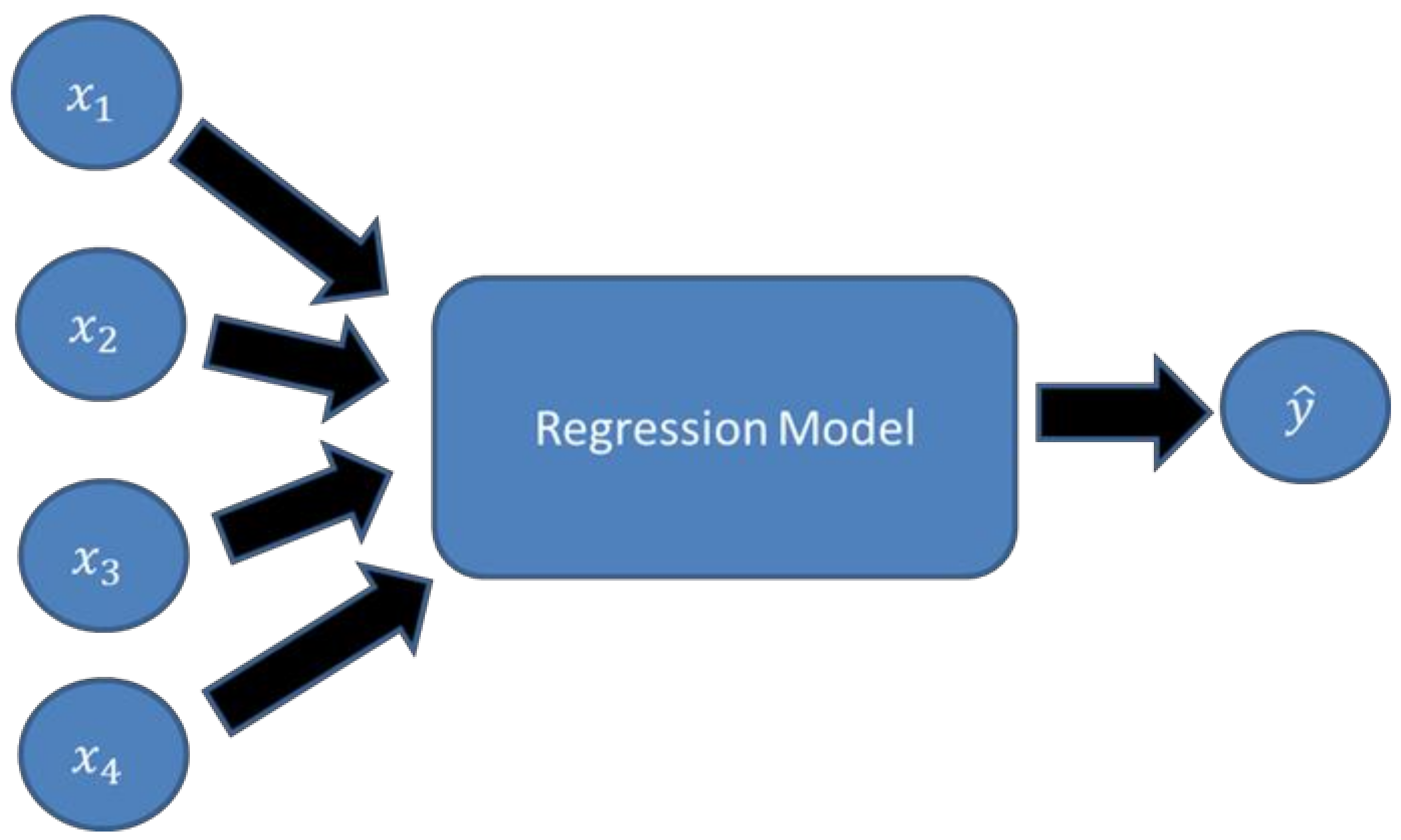
2.1. Linear and Quadratic Modeling Equations

The linear model is relatively simple with a form given in Equation (1).
y ^ = β 0 + i = 1 n β i x i
where y ^ is the predicted value for output variable y , the x i terms are the input values (there are n different inputs with subscripts i) and the β values are fitted parameters. Considering a quadratic expression, there will be a number of additional terms:
y ^ = β 0 + i = 1 n β i x i + i = 1 n j = i n β i j x i x j
Including the linear terms from Equation (1) in addition to pair-wise combinations of different inputs, which can lead to a large number of terms and a large number of additional parameters β i j , which need to be fitted.

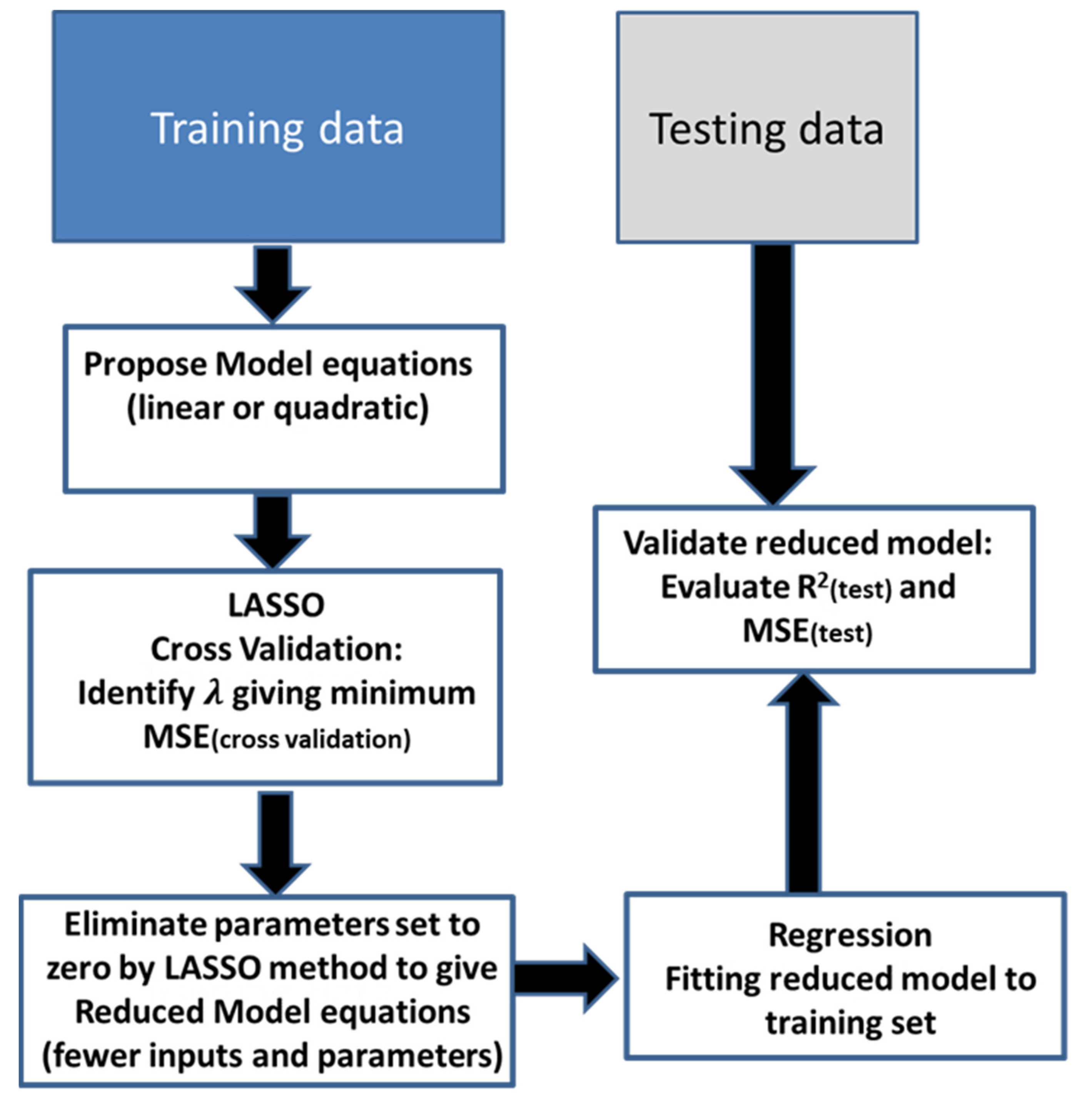
2.2. Model Reduction through LASSO Shrinkage

The most common method used for regression is the least squares formulation, which aims to minimize the residual sum of squares (RSS):
R S S = z = 1 N y z y ^ z 2
which is the sum of the differences between measured outputs and predicted outputs squared for N data points. Shrinkage methods attempt to reduce the magnitude of the predicted β values (shrinking them). This is performed by modifying Equation (3), adding an additional term, and in the case of LASSO shrinkage, this is given in Equation (4) [19]:
R S S = z = 1 N y z y ^ z 2 + λ i = 1 n β i
where n is the number of input variables and λ is a tuning parameter. This is related to the linear model in Equations (1) and (2) but can also be applied to quadratic expressions as follows:
R S S = z = 1 N y z y ^ z 2 + λ i = 1 n β i + λ i = 1 n j = i n β i j
such that all the parameters in the linear and quadratic terms are included together. In either case, Equations (4) or (5) are minimized during fitting, which simultaneously reduces the error between model and measured values and reduces the magnitude the β values. This is controlled by tuning the value of λ , and increasing this value should decrease the values of fitted parameters. In this case, using the LASSO formulation with absolute values of the parameters, it can be shown that this leads to increasing numbers of parameters set to zero [19]. This in turn allows parameters set to zero to be neglected together with the associated inputs producing a simplified or reduced model [19].

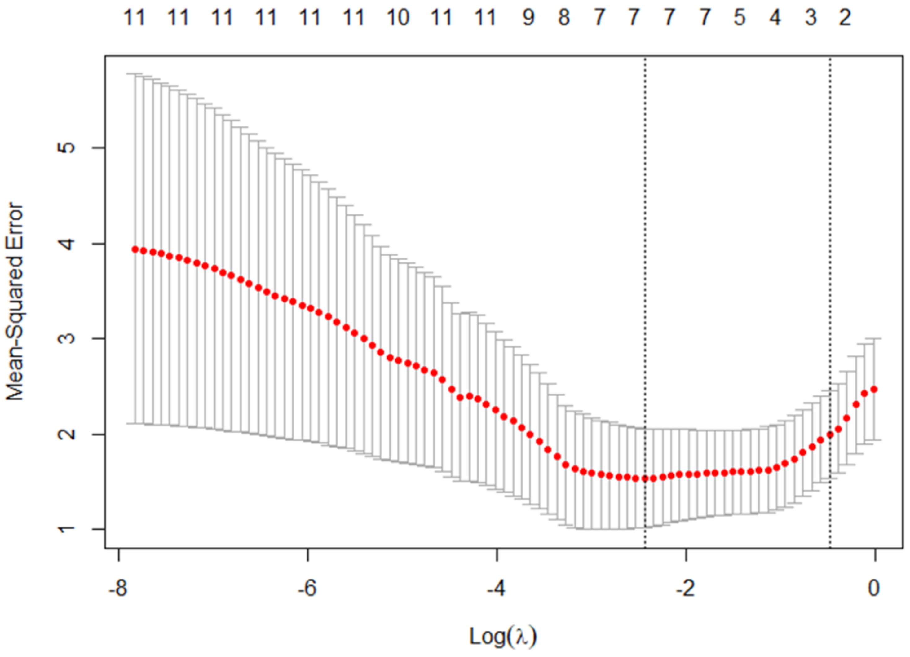
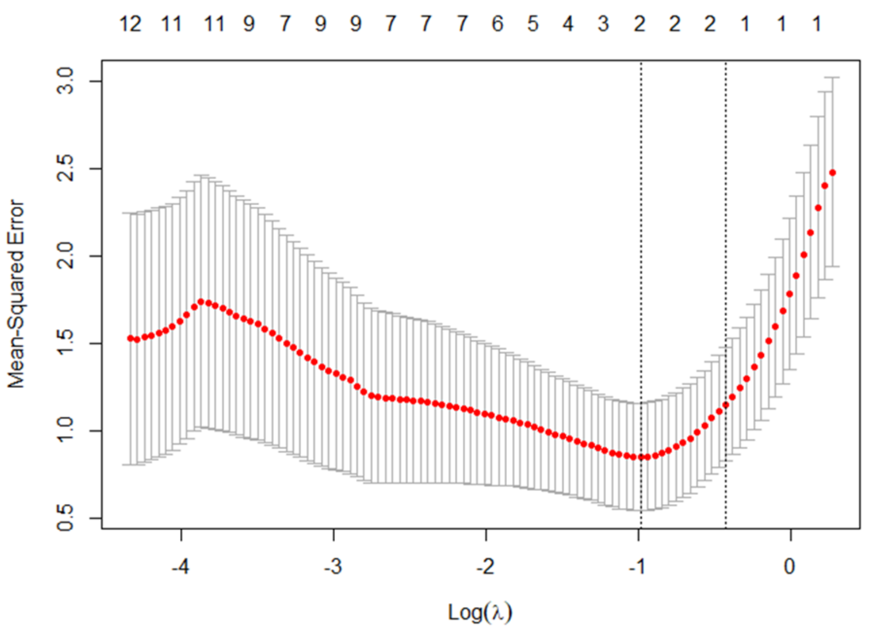
2.3. Cross Validation and Model Development
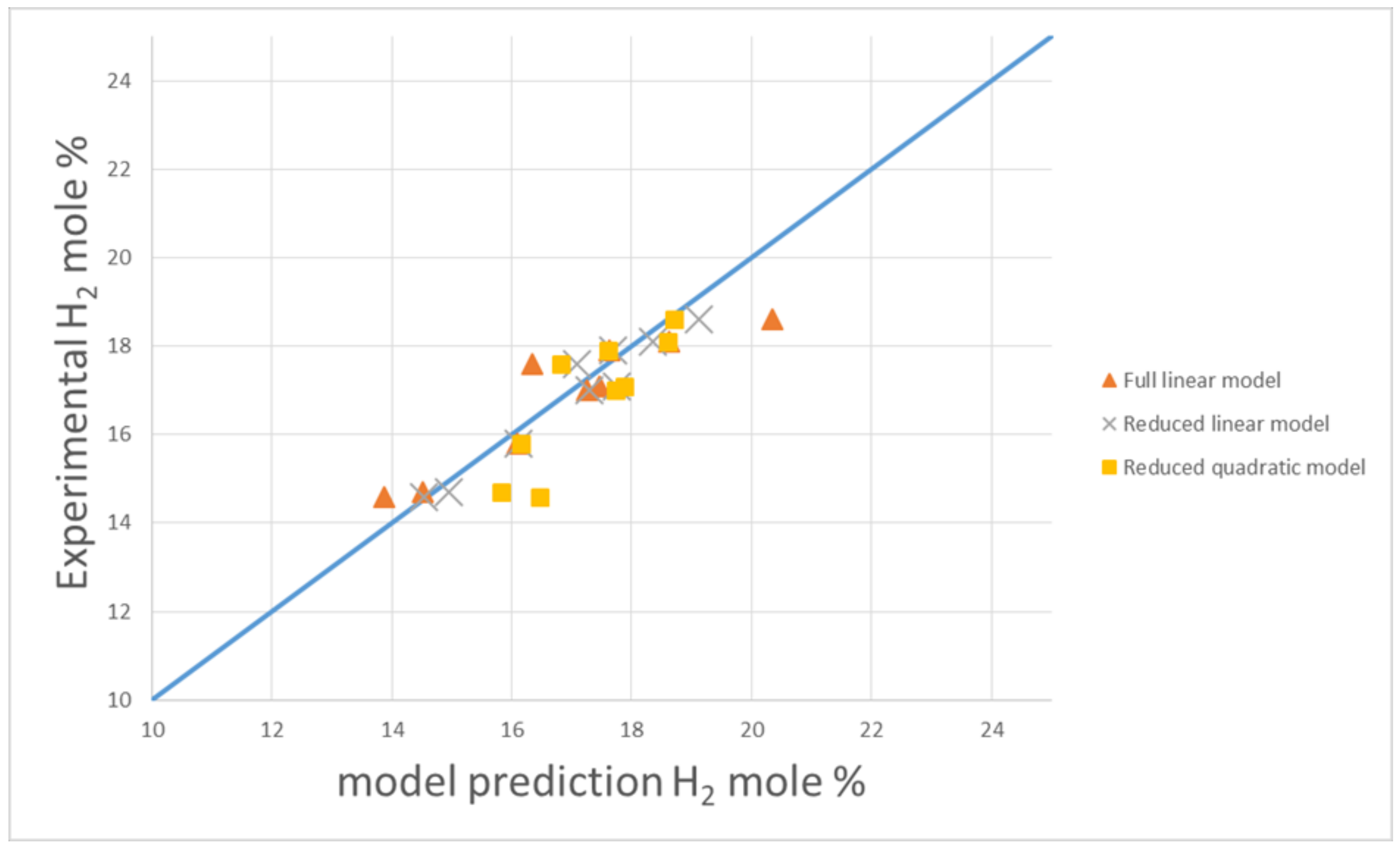
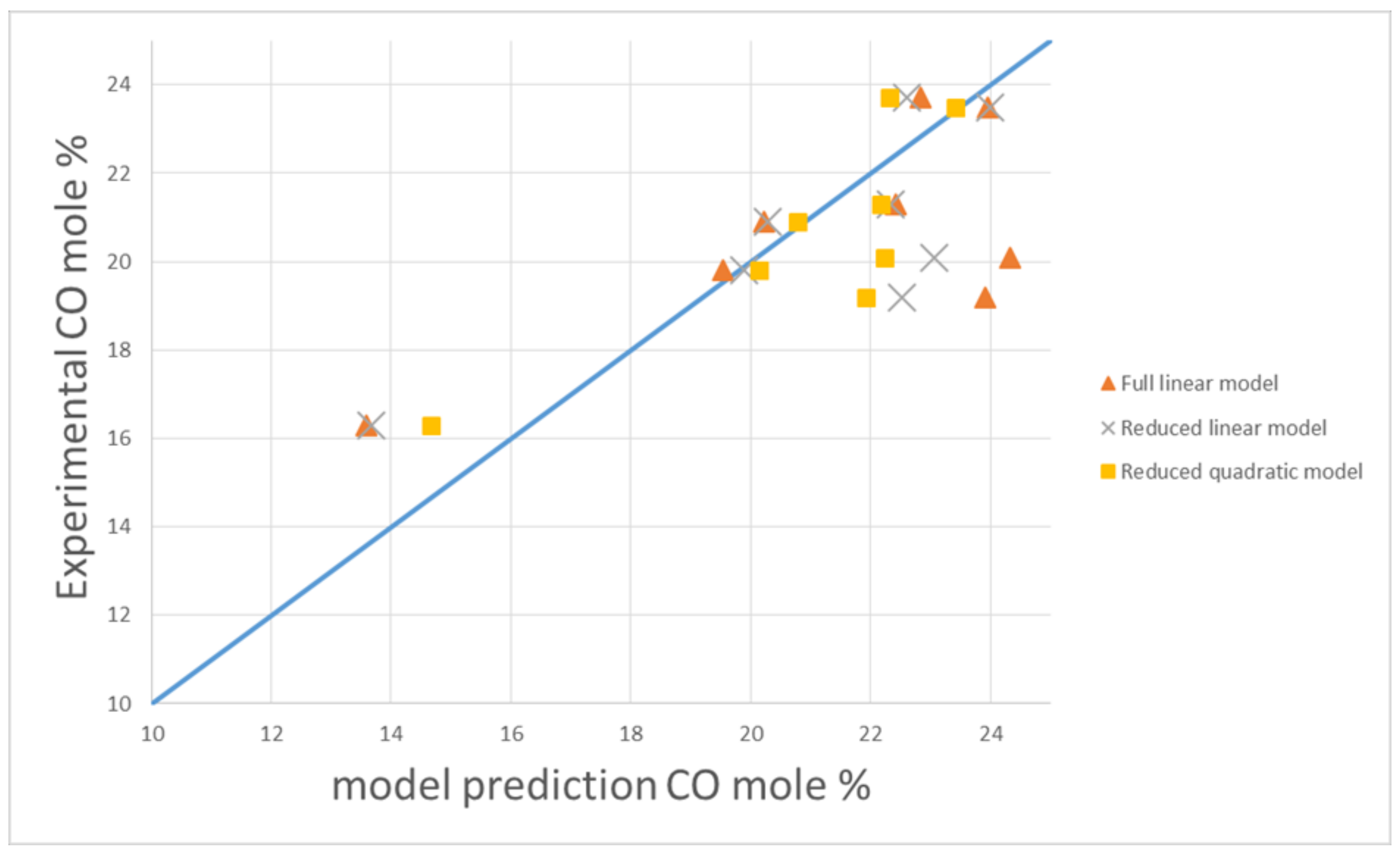
For comparison, three different types of models will be developed and tested:
  • Full linear model;
  • Reduced linear model;
  • Reduced quadratic model.
To develop these models, the procedure shown in Figure 2 was employed here for both the linear and quadratic reduced models. The available data were initially separated into separate training and testing sets. Then, only data from the training set was used in cross validation with the LASSO approach and was used to identify a λ value which minimises the cross validation MSE (mean squared error). Utilizing the LASSO method with this λ reveals which of the parameters have been set to zero and the non-zero parameters were identified to generate reduced expressions. These reduced expressions were then fitted to the full training set data giving fitted values for the identified parameters. For the full linear model, there was no cross validation and all the parameters were obtained through regression using the training set. Finally, all the fitted models were validated to see if they were able to adequately predict the results of the testing data.

3. Case Study Based on a Commercial Biomass Gasifier

The measured input and output values are taken from the study of Chee, who investigated the effect of different operating conditions and different wood-based feedstocks on the performance of a commercial biomass downdraft gasifier [12]. In particular, the gasifier used by Chee had a rotating grate at the base of the fixed bed and a fan for driving the air flow and the rotation rate of these two components were investigated [12]. This data set consists of 34 data points with input values given in Table 1 [12]. Run number “201” in this study was not used here because the conditions for that run were significantly different from all the others tested (with an equivalence ratio of 0.56) [12]. From these 34 data points, 25 randomly chosen points were assigned to the training set and the remaining 9 data points were used for testing. The data values used are also given in the Supplementary data file together with additional data used for validation and all the model parameters.
These data values are used to predict the produced gas properties:
  • Hydrogen (mole %);
  • Carbon monoxide (mole %);
  • Carbon dioxide (mole %);
  • Methane (mole %);
  • Nitrogen (mole %);
  • Gas/fuel ratio (kg/kg).

3.1. Cross Validation and Model Development

Cross validation and fitting with the LASSO approach was carried out here using the statistical software R and RStudio using the package “glmnet” written by Friedman et al. [20]. This software is commonly used for both linear and non-linear regression in addition to classification. To make this easier, various packages and subroutines have been written in this software including machine learning-based methods such as the LASSO. In the field of process/chemical engineering, alternative software such as Aspen Plus is a very powerful tool which can be used for both simulation and regression of parameters for both linear and non-linear expressions but as far as we know it does not include the option to include shrinkage-based model reduction (although perhaps subroutines could be written to add this functionality in the future).
An example of the output of cross validation is shown in Figure 3, which demonstrates how the mean square error (from cross validation) varies with changing the value of the tuning parameter λ . This particular graph shows the cross validation results for the prediction of hydrogen mole % in the produced gas based on a linear expression in terms of the 11 inputs. It can be seen from the number at the top edge that the number of inputs included in the model reduces as λ increases, with a minimum MSE value given with 7 out of 11 inputs.
In particular, the inputs that can be eliminated are shown from the data to be: C, H, Fs, and bulk, so the reduced linear expression can be stated as
H 2 % = β 0 + β 1 T g a s + β 2 E R + β 3 M C + β 4 O + β 5 A s h + β 6 G r + β 7 v o i d
If starting from a quadratic expression, it might be expected that a larger number of inputs or combinations of inputs would result. However, the cross validation in Figure 4 shows a minimum MSE located near the point where there are only two inputs. Looking at the data, the two remaining terms after this point are TgasER, the product of gasification temperature and equivalence ratio, and MCAsh, the product of moisture content and ash content, suggesting that a very simple expression can be obtained:
H 2 % = β 0 + β 1 T g a s E R + β 2 M C A s h
Although, at the exact minimum, a third product, ERGr (the product of equivalence ratio and grate rotation speed), and fourth, Ovoid (the product of elemental oxygen content and the void fraction), also appear.
H 2 % = β 0 + β 1 T g a s E R + β 2 M C A s h + β 3 E R G r + β 4 O v o i d
Thus, it appears in the case of hydrogen that a quadratic expression with four terms provides a much simpler model than both the full linear model and the reduced linear model. Based on similar analysis, applying cross validation and fitting the resulting expressions to the training data, the following expressions are given in Table 2.

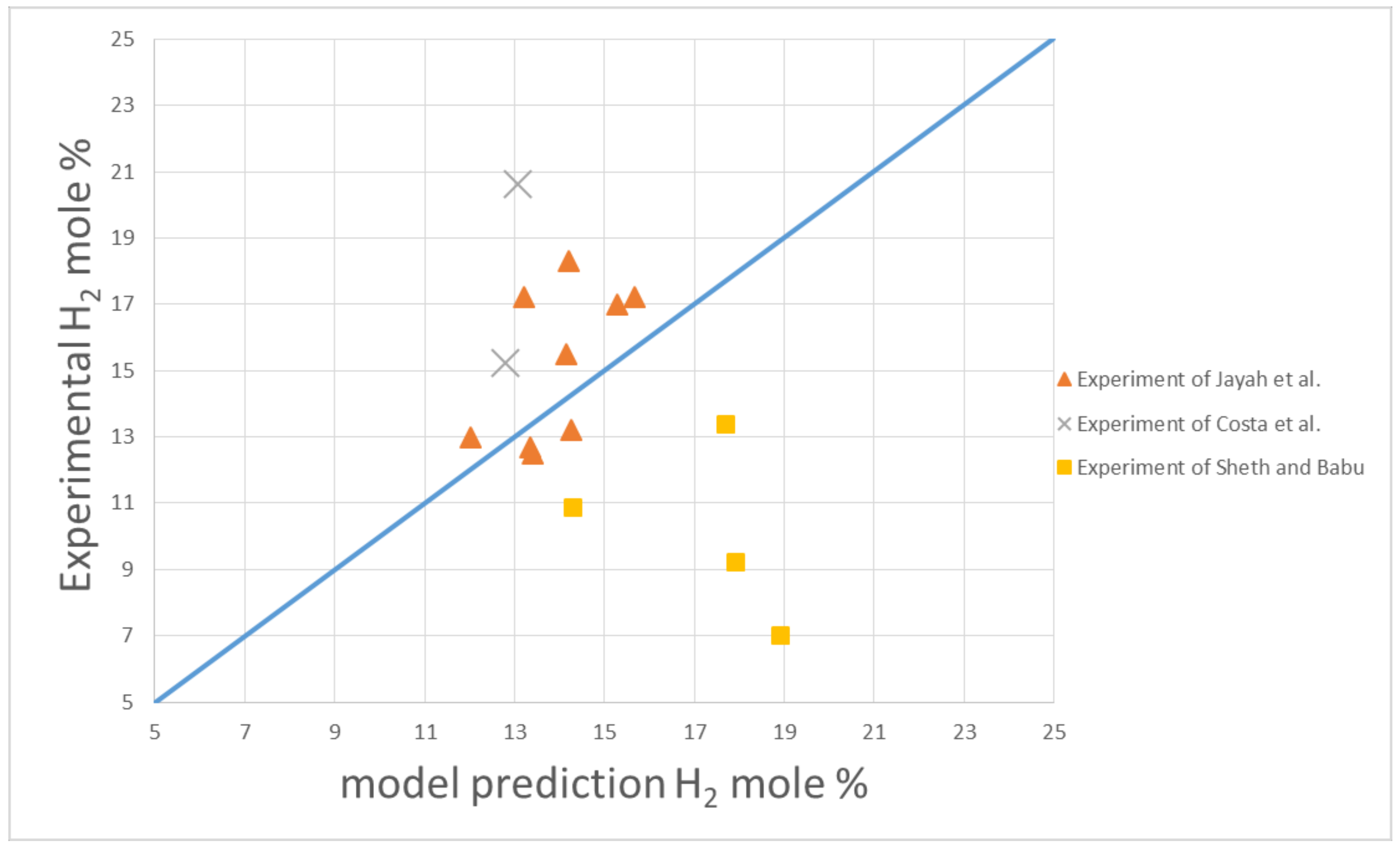
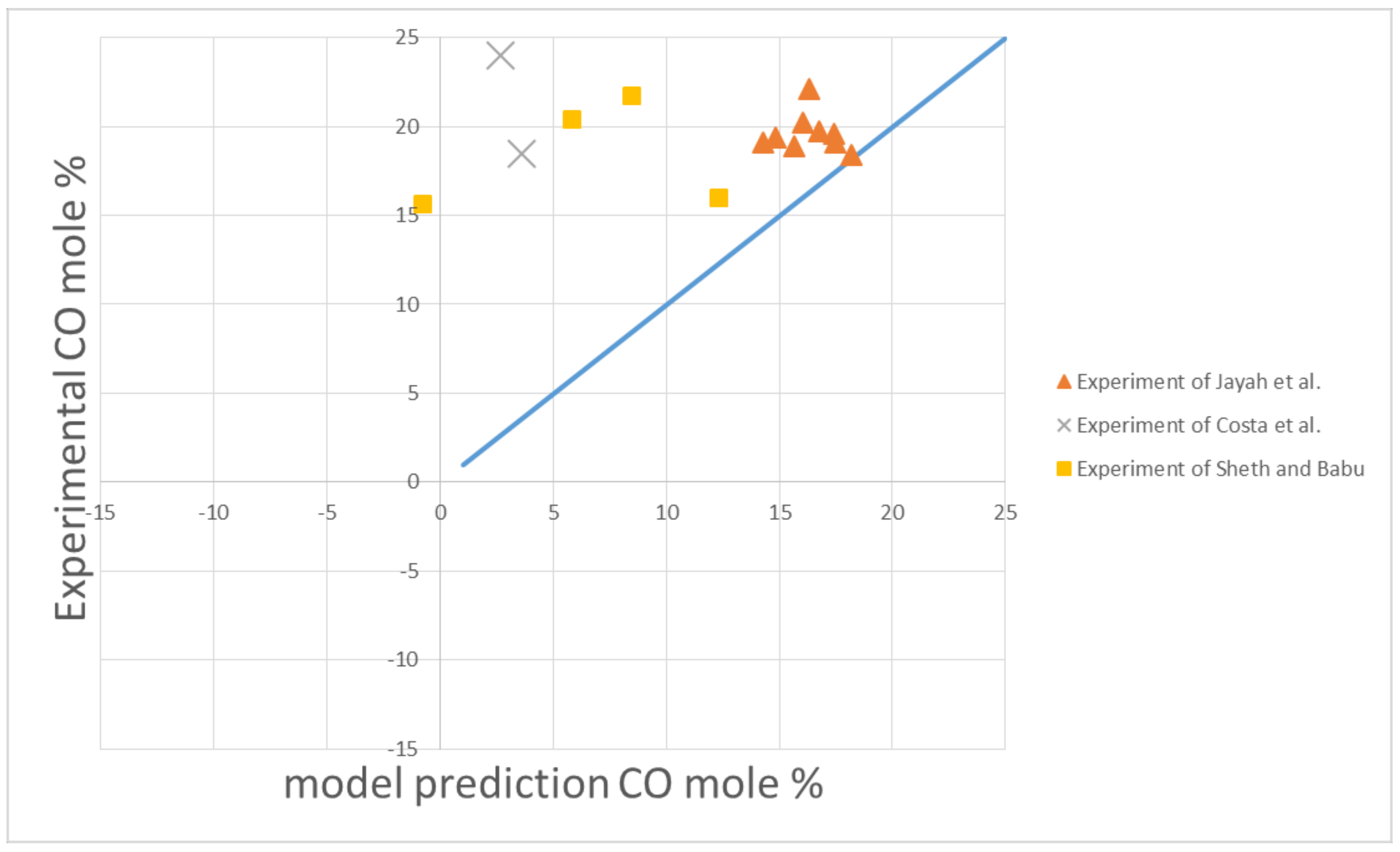
3.2. Model Validation

To evaluate the predictive power of the different models developed in Section 3.1, which are developed and trained using the training set (25 data points), they are also validated here through comparison with the testing set of data (9 data points). The performance of the different models was evaluated based on comparison of the mean squared error (MSE) and the R2 values of each model with respect to the output values from the test set as shown in Table 3. It can be seen that while the full linear model can adequately predict the output for some of the predicted outputs in almost all cases, the reduced linear or quadratic models are shown to more accurately have predictions with higher R2 and lower MSE values. An exception to this rule is the gas-to-fuel ratio, for which the full linear model has the best fit and where all the models are shown to have very high accuracy.
It is also worth noting that the model for carbon monoxide (CO) shows a very poor prediction using the full linear model and appears to require a quadratic model to obtain a reasonable predictive power. Previous studies of Mirmoshtaghi et al. [15] and Pio and Tarelho [4] have also shown difficulty fitting empirical models to the CO output of circulating and bubbling fluidized bed reactors with R2 values of 0.53 and 0.23, respectively. In this study, an R2 value of 0.513 was found for the downdraft gasifier data used here.
The fitting of these models is also demonstrated in Figure 5 and Figure 6, which show the comparison of experimental values plotted against model predictions for the test data set. This shows that all of the models appear to predict hydrogen mole percentage reasonably well, but there are some deviations for model predictions of carbon monoxide mole percentage. The reduced models are shown to give predictions closer to the experimental values for both of these outputs.
To assess if the models generated based on fitting to the data of Chee [12] can be used for other biomass gasifiers, the best fitting models for predicting hydrogen and carbon monoxide are compared against experimental data from three other downdraft gasifier studies. In particular, this experimental data includes the gasification of rubberwood (nine data points) from the study of Jayah et al. [21], the gasification of sesame wood (four data points) from the study of Sheth and Babu [22], and the gasification of wood chips (two data points) from the study of Costa et al. [23].
Figure 7 and Figure 8 show the parity plots of the reduced linear models against these three sets of data. It can be seen that the model gives a reasonable prediction of the data points from the study of Jayah et al. but has much lower accuracy for predicting the results of Costa et al. and Sheth and Babu.
Considering the reduced quadratic model, which gives the best fit to the data of Chee, when this is compared against other experimental data in Figure 9 it is shown to give poor or very poor predictions. These inaccuracies may be because of differences in the design of different downdraft gasifiers or because the conditions are outside the ranges given in Table 1. In particular, the bulk density of biomass used in all these cases are higher than those for the experiments of Chee. Additionally, these new data sources do not include grate or fan rotation speeds, so the average values from Table 1 have been assumed to utilize the reduced linear and quadratic expressions given in Table 2. Due to the second order terms in the quadratic expression, the errors associated with these assumptions lead to a much greater inaccuracy.
This shows that these empirical models may only be practical for gasifiers with a similar scale and design and within the range of conditions used to build the models. This is supported by the results of Pio and Tarelho, who also found difficulty fitting empirical models to a wide range of different gasifier data sources [4], and by Baruah et al., who suggest that data must be taken from very similar scale gasifiers and with similar feedstocks [7]. However, if a large amount of data are collected from a single biomass gasifier with different conditions and feedstocks, this methodology should provide accurate models. Furthermore, due to the LASSO model reduction applied, simpler models can be obtained with much fewer parameters, which are very practical for the design of similar gasifiers.

4. Conclusions

Empirical models are proposed for the prediction of downdraft biomass gasifiers’ outlet values (in particular the product gas composition). Both linear and quadratic expressions are considered, and a model reduction method is implemented based on cross validation with the LASSO method in order to select subsets of important parameters so that the resulting expressions can be simplified. This identifies significant parameters and reduces the number of parameters which must be regressed. We believe this is the first application of this LASSO model reduction method in the field of biomass gasification which is generally formulated in terms of linear models (combining Equations (1) and (4)) [19] but can also be used for more complex quadratic equations (see Equations (2) and (5)), as demonstrated here.
This model reduction is particularly important for quadratic expressions which can contain a large number of parameters. For example, in the case study considered here, there are 11 inputs and a quadratic expression including all combinations of these 11 (as in Equation (2)) would have 78 different parameters to fit, but following the model reduction in the case study, there were 5–10 parameters needing to be identified. Considering the training data set contained only 25 data points, this means fitting the full quadratic expression with 78 parameters would not have been feasible.
In addition to reducing the complexity of fitted correlations, it is shown here that in almost all the outputs in the case study, the model reduction also leads to improved model prediction accuracy when the models were evaluated using test set data (which has not been used for training the models).

Supplementary Materials

The following are available online at https://www.mdpi.com/article/10.3390/su132112191/s1, Excel data file including “experimentaldatafull” tab containing experimental data gathered from [12,21,22,23], “fig5+fig6” tab containing the data used to plot Figure 5 and Figure 6, “fig7+fig8+fig9 data” tab containing data used to plot Figure 7, Figure 8 and Figure 9, and “fitted reduced model parameters” tab containing the fitted parameters for the models given in Table 2.

Author Contributions

Conceptualization, M.B. and H.M.U.A.; methodology, M.B.; validation, M.B.; data curation, M.B.; writing—original draft preparation, M.B.; writing—review and editing, M.B. All authors have read and agreed to the published version of the manuscript.

Funding

This research received no external funding.

Institutional Review Board Statement

Not applicable.

Informed Consent Statement

Not applicable.

Data Availability Statement

Experimental data used to build models can be found in [12], and data and models can also be found in the Supplementary file and in [21,22,23].

Acknowledgments

Support is acknowledged from the SRD scholarship, Dongguk University-Seoul, Seoul, South Korea.

Conflicts of Interest

The authors declare no conflict of interest.

References

  1. Patra, T.K.; Sheth, P.N. Biomass gasification models for downdraft gasifier: A state-of-the-art review. Renew. Sustain. Energy Rev. 2015, 50, 583–593. [Google Scholar] [CrossRef]
  2. Safarian, S.; Saryazdi, S.M.E.; Unnthorsson, R.; Richter, C. Artificial neural network integrated with thermodynamic equi-librium modeling of downdraft biomass gasification-power production plant. Energy 2020, 213, 118800. [Google Scholar] [CrossRef]
  3. Marcantonio, V.; Ferrario, A.M.; Di Carlo, A.D.; Del Zotto, L.; Monarca, D.; Bocci, E. Biomass Steam Gasification: A Comparison of Syngas Composition between a 1-D Matlab Kinetic Model and a 0-D Aspen Plus Quasi-Equilibrium Model. Comput. 2020, 8, 86. [Google Scholar] [CrossRef]
  4. Pio, D.T.; Tarelho, L.A.D.C. Empirical and chemical equilibrium modelling for prediction of biomass gasification products in bubbling fluidized beds. Energy 2020, 202, 117654. [Google Scholar] [CrossRef]
  5. Ferreira, S.; Monteiro, E.; Brito, P.; Vilarinho, C. A Holistic Review on Biomass Gasification Modified Equilibrium Models. Energies 2019, 12, 160. [Google Scholar] [CrossRef] [Green Version]
  6. Ayub, H.M.U.; Park, S.J.; Binns, M. Biomass to Syngas: Modified Non-Stoichiometric Thermodynamic Models for the Downdraft Biomass Gasification. Energies 2020, 13, 5668. [Google Scholar] [CrossRef]
  7. Baruah, D.; Baruah, D.C.; Hazarika, M.K. Artificial neural network based modeling of biomass gasification in fixed bed downdraft gasifiers. Biomass- Bioenergy 2017, 98, 264–271. [Google Scholar] [CrossRef]
  8. Pandey, D.S.; Das, S.; Pan, I.; Leahy, J.J.; Kwapinski, W. Artificial neural network based modelling approach for municipal solid waste gasification in a fluidized bed reactor. Waste Manag. 2016, 58, 202–213. [Google Scholar] [CrossRef] [PubMed] [Green Version]
  9. Mutlu, A.Y.; Ozgun, Y. An artificial intelligence based approach to predicting syngas composition for downdraft biomass gasification. Energy 2018, 165, 895–901. [Google Scholar] [CrossRef]
  10. Puig-Arnavat, M.; Hernández, J.A.; Bruno, J.C.; Coronas, A. Artificial neural network models for biomass gasification in fluidized bed gasifiers. Biomass Bioenergy 2013, 49, 279–289. [Google Scholar] [CrossRef]
  11. Chavan, P.D.; Sharma, T.; Mall, B.K.; Rajurkar, B.D.; Tambe, S.S.; Sharma, B.K.; Kulkarni, B.D. Development of data-driven models for fluidized-bed coal gasification process. Fuel 2012, 93, 44–51. [Google Scholar] [CrossRef]
  12. Chee, C.S. The Air Gasification of Wood Chips in a Downdraft Gasifier. Master’s Thesis, Kansas State University, Manhattan, KS, USA, 1987. [Google Scholar]
  13. Pradhan, P.; Arora, A.; Mahajani, S.M. A semi-empirical approach towards predicting producer gas composition in a biomass gasification. Bioresour. Technol. 2019, 272, 535–544. [Google Scholar] [CrossRef] [PubMed]
  14. Rupesh, S.; Muraleedharan, C.; Arun, P.V. A comparative study on gaseous fuel generation capability of biomass materials by thermo-chemical gasification using stoichiometric quasi-steady-state model. Int. J. Energy Environ. Eng. 2015, 6, 375–384. [Google Scholar] [CrossRef] [Green Version]
  15. Mirmoshtaghi, G.; Skvaril, J.; Campana, P.E.; Li, H.; Thorin, E.; Dahlquist, E. The influence of different parameters on bio-mass gasification in circulating fluidized bed gasifiers. Energy Convers. Manag. 2016, 126, 110–123. [Google Scholar] [CrossRef]
  16. Gil, M.V.; Gonzalez-Vasquez, M.P.; Garcia, R.; Rubiera, F.; Pevida, C. Assessing the influence of biomass properties on the gasification process using multivariate data analysis. Energy Convers. Manag. 2019, 184, 649–660. [Google Scholar] [CrossRef]
  17. Dellavedova, M.; Derudi, M.; Biesuz, R.; Lunghi, A.; Rota, R. On the gasification of biomass: Data analysis and regressions. Process. Saf. Environ. Prot. 2012, 90, 246–254. [Google Scholar] [CrossRef]
  18. Pan, I.; Pandey, D.S. Incorporating uncertainty in data driven regression models of fluidized bed gasification: A Bayesian approach. Fuel Process. Technol. 2016, 142, 305–314. [Google Scholar] [CrossRef] [Green Version]
  19. James, G.; Witten, D.; Hastie, T.; Tibshirani, R. An Introduction to Statistical Learning with Applications in R, 2nd ed.; Casella, G., Fienberg, S., Olkin, I., Eds.; Springer: New York, NY, USA, 2013; pp. 59–126. [Google Scholar]
  20. Friedman, J.; Hastie, T.; Narasimhan, B.; Simon, N.; Tay, K.; Tibshirani, R. glmnet package for generalized linear models. Available online: https://glmnet.stanford.edu (accessed on 28 September 2021).
  21. Jayah, T.H.; Aye, L.; Fuller, R.J.; Stewart, D.F. Computer simulation of a downdraft wood gasifier for tea drying. Biomass-Bioenergy 2003, 25, 459–469. [Google Scholar] [CrossRef]
  22. Sheth, P.N.; Babu, B.V. Experimental studies on producer gas generation from wood waste in a downdraft biomass gasifier. Bioresour. Technol. 2009, 100, 3127–3133. [Google Scholar] [CrossRef] [PubMed]
  23. Costa, M.; La Villetta, M.; Piazzullo, D.; Cirillo, D. A Phenomenological Model of a Downdraft Biomass Gasifier Flexible to the Feedstock Composition and the Reactor Design. Energies 2021, 14, 4226. [Google Scholar] [CrossRef]
Figure 1. Simple schematic of a regression model used to take inputs x and calculate a predicted output value y ^ .
Sustainability 13 12191 g001
Figure 2. Procedure used to develop and validate reduced linear and quadratic models.
Sustainability 13 12191 g002
Figure 3. Plot of cross validation MSE against the log of the tuning parameter λ from Equation (4) for the prediction of hydrogen % using a linear expression. The numbers above the graph show the corresponding number of inputs with non-zero parameters.
Sustainability 13 12191 g003
Figure 4. Plot of cross validation MSE against the log of the tuning parameter λ from Equation (5) for the prediction of hydrogen % using a quadratic expression. The numbers above the graph show the corresponding number of terms with non-zero parameters in the quadratic model.
Sustainability 13 12191 g004
Figure 5. Parity plot of models against experimental hydrogen mole % using data from Chee [12].
Sustainability 13 12191 g005
Figure 6. Parity plot of models against experimental carbon monoxide mole % using data from Chee [12].
Sustainability 13 12191 g006
Figure 7. Parity plot of reduced linear model against experimental hydrogen mole % for data from other downdraft biomass gasifiers using experimental data from the literature [21,22,23].
Sustainability 13 12191 g007
Figure 8. Parity plot of reduced linear model against experimental carbon monoxide mole % for data from other downdraft biomass gasifiers using experimental data from the literature [21,22,23].
Sustainability 13 12191 g008
Figure 9. Parity plot of reduced quadratic model against experimental carbon monoxide mole % for data from other downdraft biomass gasifiers using experimental data from the literature [21,22,23].
Sustainability 13 12191 g009
Table 1. Input parameters, ranges, and average values for a commercial downdraft biomass gasifier using data from Chee [12].
Gasifier InputRangeAverage
Tgas = Gasification temperature (K)961–11001039
ER = Equivalence ratio0.1555–0.26070.2001
MC = Moisture content (% wet basis)5.4–22.411.3
H = Hydrogen content (% dry basis)47.88–49.4448.53
O = Oxygen content (% dry basis)5.78–6.005.9
C = Carbon content (% dry basis)39.06–44.3143.44
Ash = Ash content (% dry basis)1.10–2.071.66
Gr = Grate rotation speed (rph)2.55–20.695.13
Fs = Gas fan speed (rpm)1388–25611750
Bulk = Wet bulk density (kg/m3)133–230167.35
Void = Biomass void percent (%)32–5646.22
Table 2. Reduced model expressions resulting from cross validation with the LASSO approach.
Reduced Linear ModelReduced Quadratic Model
H 2 % = β 0 + β 1 T g a s + β 2 E R + β 3 M C + β 4 O + β 5 A s h + β 6 G r + β 7 v o i d H 2 % = β 0 + β 1 T g a s E R + β 2 M C A s h + β 3 E R G r + β 4 O v o i d
C O % = β 0 + β 1 T g a s
+ β 2 E R + β 3 M C
+ β 4 O + β 5 A s h
+ β 6 G r + β 7 F s + β 8 b u l k
+ β 9 v o i d
C O % = β 0 + β 1 T g a s O
+ β 2 E R O + β 3 E R A s h
+ β 4 E R b u l k + β 5 M C G r
+ β 6 H O + β 7 A s h G r + β 8 F s b u l k
C O 2 % = β 0 + β 1 E R
+ β 2 M C + β 3 O
+ β 4 A s h + β 5 G r
+ β 6 F s + β 7 b u l k + β 8 v o i d
C O 2 % = β 0 + β 1 O
+ β 2 T g a s E R + β 3 T g a s O
+ β 4 M C A s h + β 5 M C G r  
+ β 6 M C b u l k + β 7 O v o i d + β 8 F s b u l k + β 9 b u l k v o i d
C H 4 % = β 0 + β 1 E R
+ β 2 M C + β 3 C
+ β 4 H + β 5 A s h  
+ β 6 G r + β 7 F s + β 8 v o i d
C H 4 % = β 0 + β 1 T g a s G r
+ β 2 E R A s h + β 3 E R v o i d
+ β 4 M C A s h + β 5 M C F s  
+ β 6 C C + β 7 H v o i d + β 8 G r b u l k
N 2 % = β 0 + β 1 E R
+ β 2 M C + β 3 C
+ β 4 G r + β 5 v o i d
N 2 % = β 0 + β 1 T g a s E R
+ β 2 E R O + β 3 E R G r
+ β 4 M C A s h + β 5 M C v o i d
G / F = β 0 + β 1 E R
+ β 2 C + β 3 H
+ β 4 O + β 5 G r + β 6 F s + β 7 v o i d
G / F = β 0 + β 1 C
+ β 2 T g a s O + β 3 E R H
+ β 4 E R F s + β 5 E R v o i d  
+ β 6 C C + β 7 C H + β 8 O O + β 9 G r b u l k
Table 3. Validation of models against a testing set of data showing the prediction capability of full linear and reduced linear and quadratic models.
Gasifier Input1H2COCO2CH4N2G/F
Full linear model# terms111111111111
MSE(test)0.6486.8691.0430.0375.1040.0025
R20.660−0.0090.6490.7530.4400.953
Reduced linear model# terms798857
MSE(test)0.1464.8500.8000.0100.5020.0032
R20.9240.2880.7310.9350.9450.942
Reduced quadratic model# terms489859
MSE(test)0.7773.3170.8300.0111.2320.0031
R20.5920.5130.7200.9280.8650.943
Publisher’s Note: MDPI stays neutral with regard to jurisdictional claims in published maps and institutional affiliations.

