The Effectiveness of Environmental Spending in China and the Environmental Kuznets Curve

Abstract

The aim of this study is to determine whether recent environmental spending in China has enabled it to reduce its emissions of greenhouse gases in the context of an Environmental Kuznets Curve-based model and promote sustainable economic development. Following the Paris Agreement in 2015, there has been a coordinated effort to reduce the consumption of fossil fuels and prevent the excessive warming of the climate. The study uses annual regional data across China and a dynamic panel data approach for estimating an EKC model which includes measures of the increased use of fossil fuels and the spending across China to reduce environmental damage. The results suggest that the policies have been effective in controlling emissions across a variety of pollutants and that the EKC tends to hold in China but varies according to the pollutant. This suggests that these policies should be continued and where possible, extended.

1. Introduction

There is an increasing demand for countries across the world to reduce their pollution in general and fossil fuel use in particular. Since the Paris Agreement in 2015, countries around the world have agreed to reduce fossil fuel use and ensure that the temperature doesn’t rise by more than 2 degrees relative to pre-industrial levels. China is currently one of the fastest growing economies in the world and is also a major producer of greenhouse gases, and to limit the growth in emissions it has implemented policies to ensure that these emissions are more controlled over the next few decades. The aim of this study is to estimate a model including measures of the recent environmental-spending policies in China, in the context of the Environmental Kuznets Curve model (EKC).

This study uses an applied approach to analysing the effectiveness of environmental expenditure from the perspective of government-based spending and the levels of investment to determine which has worked best to date, in the context of the EKC model. We have not sought to add a new model to the study; the analysis is based on the standard EKC model, augmented by energy consumption, trade and population effects, but we have also added to the approach the environmental-spending measures, which is the first time this has been done in this context, as far as we know. This study aims to contribute to the current literature in three main respects: firstly, by incorporating the environmental-spending measures and investment in the environment into a standard EKC model. In addition, we assessed the importance of these measures across a wide range of pollutants that have not been studied in such detail before. Thirdly, we used dynamic panel models to account for the partial adjustment that is inherent in pollutant-based models, using both the Arellano—Bond and Arellano—Bover approaches to ensure the results are robust.

It is has been well established that there is an association between sustainable economic development and environmental deterioration since the initial study of Grossman and Krueger (1991). This relationship is most commonly conceptualised through the EKC, and there has been a wide range of methodologically diverse research conducted on it, with many of these studies illustrating the serious impact pollution has on the economy and the existence of the EKC relationship [1,2]. There have also been studies specifically on China which support the existence of the EKC, such as [3,4]. So, the use of this model is important when analysing the environment.

Following the introduction, the first section contains the literature review on the EKC, including its development and both international and Chinese research. The second section focuses on describing the Chinese provincial data and discussing the methodology used. We then analyse the results and finally offer some conclusions and explore the policy implications.

2. Literature Review

2.1. The Genesis of the EKC

With the rise in environmental awareness in the second half of the 20th century, research on environmental economics began to attract more interest, leading to the development of the EKC hypothesis, which explores how economic growth can affect environmental degradation. The initial study considered the environmental impacts of economic growth in NAFTA and conducted an empirical study with reduced-form regression models between income per capita and air pollutant emissions [5,6]. Panayotou [7] linked the inverted U-shaped curve with the Kuznets Curve [8], naming it the Environmental Kuznets Curve for its similarity. The shape can be flattened if environmentally harmful subsidies are removed [7]. More popular discussions began with the World Bank Development Report [9], this background paper verifies the existence of an inverted U-shaped relationship between income levels and air pollutant emissions, including sulfur dioxide and suspended particulates emissions [10]. Moreover Grossman and Krueger [6] used a panel data model analysis with more comprehensive environmental indicators in GEMS and found further evidence of inverted U-shaped type relationships. From this they were able to calculate turning points at around USD 4000–8000 (Sulfur dioxide at USD 4053, smoke at USD 6151 and COD at USD 7853).

There are three mechanisms through which income can affect the environment: scale, composition and technical effects [5]. The scale effect reveals that economic growth increases with more natural resource inputs, resulting in higher relative environmental degradation. The EKC curve is split into two separate periods. The scale effect influences the rising period at the beginning, and both composition and technical effects can occur in the latter declining period of the EKC curve as income levels increase. The technical effects can be interpreted as the use of clean technology increasing productivity and facilitating transition with the aim of improving the environmental quality.

Throughout the development of the EKC theory, several criticisms and alternative theories have been raised. For example, the U-shaped curve may not be the best fit for the relationship between sustainable economic development and environmental deterioration, with an inverse N-shaped curve perhaps being a better representation, as shown by an increase in environmental deterioration after the initial period of decline.

2.2. International Research

The empirical analysis of the EKC focuses on the relationship between GDP per capita and various pollutant emissions. The research so far has included multiple comprehensive analyses, conducted across a wide range of explanatory variables to test the determinants of environmental degradation, for example, energy consumption, population characteristics, trade openness, foreign direct investment and policy indicators.

The EKC research on environmental pollutants mainly covers air pollution, water waste and solid waste. CO₂ emissions, as the main GHG contributing to global warming, are the most commonly used emissions in research on the EKC and the existence of an inverse U-shaped EKC model with CO₂ emissions is supported by a relatively large number of studies [2,11,12,13,14,15]. Research on other emissions includes sulfur dioxide emissions [6,16], and nitrogen oxide emissions [17]. EKC analysis has also considered various types of air pollution, including different types of particulate matter (such as smoke and dust, SPM and PM2.5) [18,19]. Panayotou [7] also accounts for deforestation rates in his EKC analysis, suggesting the EKC relationship has a greater impact on more populous and tropical countries. However, this is contradicted by some studies [20], whose deforestation-specific analysis of the EKC found deforestation is not beneficial for increasing the income level.

The ability to accurately estimate the turning point of the EKC depends on the scale of the study as well as the range and quality of the control variables used. The selection of explanatory variables tends to represent the objectives of their studies. For example, a study focusing on urban level data, using 276 metropolitan areas, obtained a turning point (USD 55,102) considerably higher than those found in country-level studies; thus policymakers relying solely on country-level data may be misled [21]. Apergis and Ozturk [2] considered government expenditure in their research, as well as four policy indicators: political indexes, government effectiveness, regulatory activities and the level of corruption. The first three were found to have a positive relationship with pollution, while corruption was found to be negatively associated with pollution. Al-Mulali et al. [22] found that renewable energy measures exhibit highly significant inverted-U type relationships with emissions. However, renewable energy sources should not all be treated equally; for example, although an EKC analysis based in France found nuclear energy can decrease carbon dioxide emissions across both the short and long term, the application of nuclear energy should be treated with caution because the potential risks are large and there are often high safety management costs [23]. The impact of international trade is more ambiguous. On the one hand, it can increase pollution as increased exports lead to higher production, but on the other hand, it also can bring positive effects to environment quality by facilitating pollution transfer through foreign direct investment, although this may just displace to other countries [24].

The existence of the EKC may also be affected by the levels of economic development across various regions. Most studies have proven the existence of an inverted U-shaped EKC in relatively well-developed areas, suggesting the environmental problems probably improve or reduce the levels of deterioration when total income reaches a certain level. The EU 28 countries indicate an inverse U-shaped curve in the relationship between residential energy consumption and gross domestic products [25]. However, Abid [26] obtains a monotonically increasing trend between CO₂ emissions and GDP in 41 EU countries. Other studies indicate that only Denmark and Italy provide evidence in support of EKC [27]. Most EKC analyses for single countries in the EU regions find the inverted U-shaped type relationships; for example, Germany exhibits a clear EKC pattern with regard to strong energy policies [28], and a concave relationship was found to exist in Romania over the period 1980–2010, perhaps because environmental policies tend to be enacted by democratic regimes as they have more of an incentive to reduce CO₂ emissions [12]. Some studies focus on the decline of electric power consumption relative to economic growth in four different countries (Australia, USA, China and Ghana); their evidence supports the validity of the EKC in Australia and China [29]. Furthermore, they found Australia and the USA performed better in reducing electric power consumption. However, some studies indicate that the pollution—income relationships they tested do not satisfy the inverse U-shaped curve. Global economic recession and globalisation have caused fluctuations in the pollution—income relationship since 2001, so only weak evidence for the inverted U shape is found from 1971 to 2001 [28].

Across the research, there are two main methodological approaches. Some papers focus on single-country analysis, applying time series data to test the relationship between income levels and environmental degradation, whereas multi-country studies must use a panel data model approach to test this association.

2.3. Research on China

EKC studies on China have been conducted since the beginning of the 21st century. During this time, China transitioned to a phase of relatively quick economic development, benefiting from globalisation and its stable government. Public environmental awareness nearly always follows economic growth, as once people have achieved relatively satisfactory income levels, they are able to pursue other means to attain higher living standards. The research has generally been conducted between the 1990s and the most recent year they could acquire data for, as determined by the limitations of the database or quality of the data. Most research has used provincial-level data for panel data model analysis, although some single-province or country-level studies have used time-series analysis.

The literature on the Chinese EKC hypothesis focuses on three types of environmental pollutants: air pollutants, waste water and solid waste discharges. The air pollution studies focus on the key emissions of carbon dioxides, nitrogen oxides, sulfur dioxides and dust emissions. Some EKC studies with provincial annual data and the country-level data for CO₂ emissions have shown evidence of the inverse U-shaped curve [30,31,32,33,34]. A study in Beijing, using monthly data from 2008M04 to 2016M12 to examine PM2.5 emissions, found evidence supporting the existence of the EKC in China. Additionally, they found vehicle exhaust emissions to be a contributor to emissions, whereas natural gas consumption contributes to the reduction in PM2.5 [4].

The large variety of data available in the China Statistical Yearbook gives researchers access to a variety of control variables, as required for their research objectives. Some studies also use city-level data to identify specific geographical factors in China [17,35,36] For example, He and Wang [35] introduced ‘northern city’ and ‘coastal city’ as two indicators. Technical progress has also affected the decrease of carbon emissions in China [33], which was firstly considered in the World Bank Development Report [9]. As the most populous country, the population density could be a valuable explanatory variable when analysing the pollution—income relationships. An overlapping generations (OLG) model confirms the existence of the EKC hypothesis with 10 years of provincial-level data in China, and the population growth contributes to a higher peak in this curve via simulations [37]. Finally, policy making plays an important role in pollution control. Hence, Yin [33] uses environmental regulation as a control variable to account for the moderating effect of stricter regulations on EKC.

Regarding the current studies in the EKC area, further research needs to be conducted to compare various pollutant emissions, rather than only putting the emphasis on CO₂ emissions. More needs to be done about the recent severe environmental problems in China that are mostly influenced by industrial pollution, along with the rapid economic growth. In this chapter, I conducted the analysis with three air-pollutant emissions and the COD of wastewater discharge, using China’s provincial-level data. In recent years, governments have striven to develop effective environmental policy systems; thus the effects of these policies need to be examined for their progress on pollution treatments with more empirical analyses. However, there are few EKC studies examining the determining factors behind financial inputs for environment improvements.

2.4. Environmental Spending

Although to date there has been limited analysis of the environmental-spending policy in China, there have been some studies assessing the effectiveness of fiscal policies on the environment. Zheng et al. [38] showed that environmental standards and energy-saving policies in China have reduced pollutants, based on a regional panel from 2002 to 2011. Similarly, one study] found that energy policy had reduced pollution in Shanghai based on a case study [39]. Shen et al. [40], found that the environmental policy tools available to the authorities in China were effective at improving pollution levels. Using regional data from 1997 to 2014, they also found that command and control type policies worked best.

3. Materials and Methods

3.1. Data

The Chinese regional annual data were accessed from the China Statistical Yearbook and the China Environmental Statistical Yearbook from 2004 to 2017, which consists of 31 provinces, cities and autonomous regions. The provinces are as follows: Beijing, Tianjin, Hebei, Shanxi, Inner Mongolia, Liaoning, Jilin, Heilongjiang, Shanghai, Jiangsu, Zhejiang, Anhui, Fujian, Jiangxi, Shandong, Henan, Hubei, Hunan, Guangdong, Guangxi, Hainan, Chongqing, Sichuan, Guizhou, Yunnan, Shaanxi, Gansu, Qinghai, Ningxia, Xinjiang and Tibet.

The environmental pollution variables include industrial-pollutant emissions in China, which are SO₂, CO₂, NO_x, COD and dust emissions, with all pollutant emission units measured in tons. SO₂ emissions are the major pollutant emission in terms of gaseous sulfur oxides (SO_x), which are mainly caused by industrial facilities and the burning of materials containing sulfur, releasing harmful effects into the air, as well as causing acid rain [41]. Likewise, nitrogen dioxide (NO₂) emissions can be produced from the burning of fuel in vehicles and through industrial development. The negative effects of nitrogen dioxide include acid rain and smog [41]. In China’s statistics, nitrogen oxides and dust emissions include those from industry, households, motor vehicles and centralised pollution-control facilities. Sulphur dioxide (SO₂) emissions are the total volume from industrial, household and centralised pollution-control facilities. COD was chosen as the indicator of water waste, which is from industry, agriculture, households and centralised pollution-control facilities. Nitrogen oxides and dust emissions data were only considered from 2011 to 2017 because of the lack of earlier data.

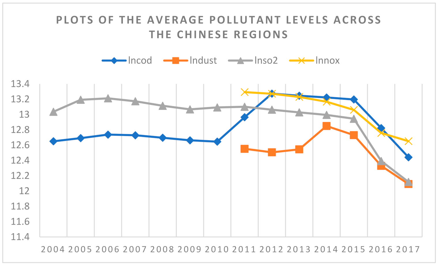
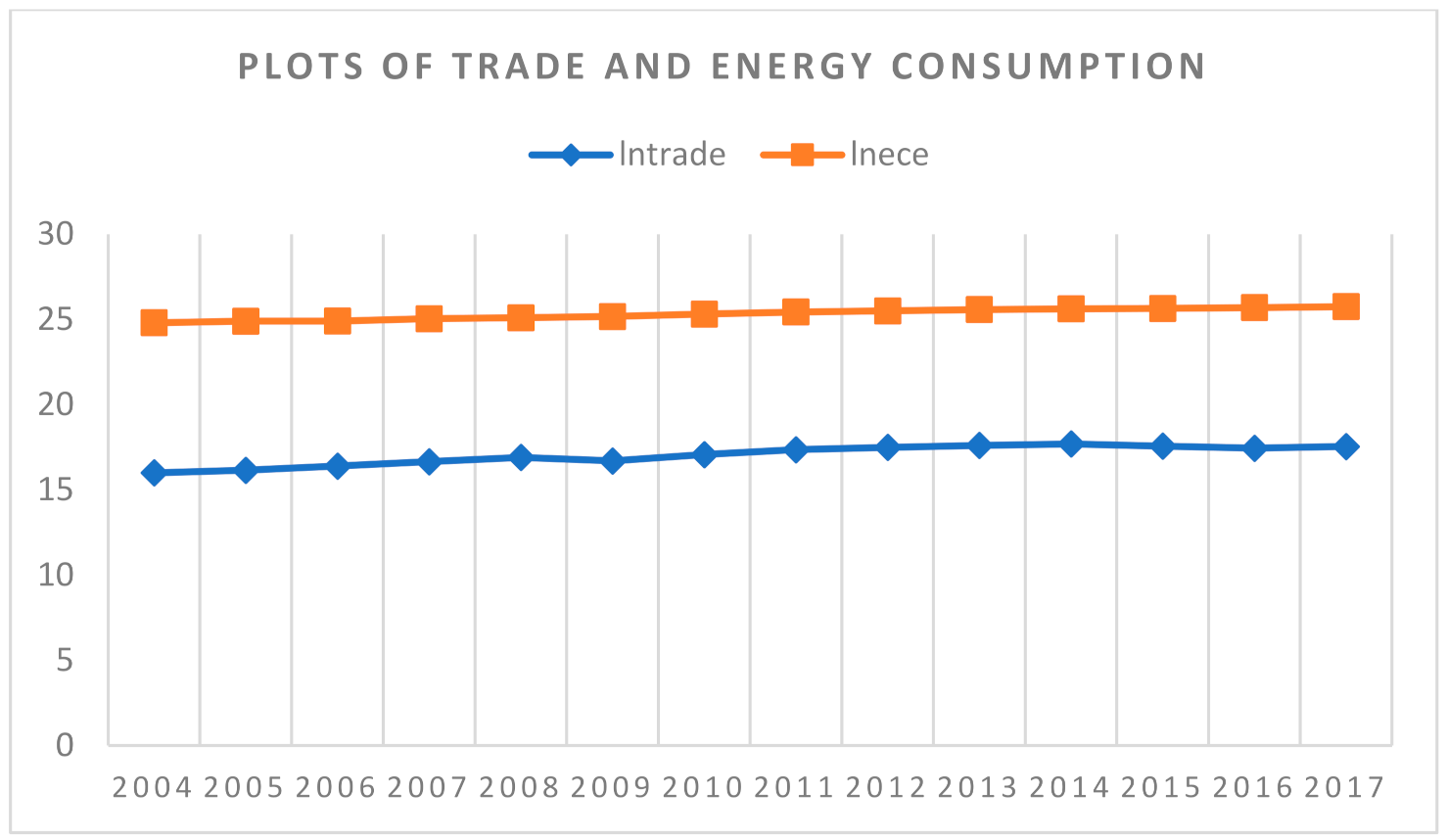
The explanatory variables for the EKC are as follows: gross domestic product (GDP) per capita measured with the Chinese domestic currency Yuan; energy consumption of electricity (ECE) measured as kilowatts per hour; population density (PD); trade openness represented by total exports and imports; local government expenditures on environmental protection; and investment in the treatment of environmental pollution, measured with Yuan as well. There is no total energy consumption for the provincial data, but electricity is the most common energy source used in China for the basic demands of households and industry. The plots of the average values for the variables across the Chinese regions are included in the Appendix A 

Table A1. Panel unit root tests.

	LLC		IPS
Variable	Level	Diff	Level	Diff
Lncod	1.290	−15.845 ** −4.875 ** −6.248 ** −3.474 **	0.790	−8.285 ** 0.855 −1.373 * −0.136
Lndust	6.473		3.850
Lnso2	12.651		11.728
Lnnox	9.636		8.246
Lngov	−8.857 **		−2.376 **
Lninv	−4.195 **		−2.462 **
Lngdppc	−15.447 **		−5.930 **
Lngdppc2	−13.045 **		−4.027 **
Lnpd	−16.870 **		−11.296 **
Lntrade	−8.760 **		−2.811 **
lnece	−9.712 **		−2.967 **

Notes: LLC is the Levin Lin and Chu test, IPS is the IM Pesaran and Shin test. A ** (*) indicates rejection of the null hypothesis at the 5% (10%) significance levels.

. All variables are in logarithmic form. There is some evidence of an inverted U-shaped curve in the pollutant data. This is particularly the case for the cod and dust pollutants, with reductions being experienced over more recent years, following changes in the laws on pollution in China. The other variables, such as government spending on the environment, have increased very little over the time frame.

3.2. Overview of Dynamic Panel Data GMM Analysis

The dynamic panel data model suits samples with a large N and small T, so we have used this approach due to only a short time period being available for the country and provincial data. The model for a dynamic panel data approach includes the lagged dependent variables as explanatory variables, but this lagged variable can result in a problem with endogeneity. This can be overcome by introducing generalised method of moments (GMM) estimators for the autoregressive model, which can be expressed as:

$$\begin{array}{ccc}{y}_{it} = \mathsf{\alpha }{y}_{it-1} + \beta x_{it} + {\epsilon }_{it};& i = 1,2,\dots , N;& t = 2,3,\dots , T\end{array}$$

(1)

where the variable $y_{it-1}$ is the lagged dependent variable, $x_{it}$ represents the other explanatory variables, ${\epsilon }_i$ is the composite error term, which is denoted as ${\epsilon }_{it}={\mu }_t+v_{it}$, containing individual effects and time-varying disturbances.

Both the Arellano—Bond (1991) [42], andArellano—Bover (1995) [43], GMM estimators can be applied with dynamic data panel models. The Arellano—Bond approach removes the error term’s relationship with the fixed effects through first difference transformations, but the transformed results cannot be obtained if there are missing values. An alternative approach is the Arellano—Bover estimator, which uses an orthogonal deviation transformation for unbalanced panels which considers additional moment conditions. The results with two transformations are robust because the dynamic panel data analysis has been considered with improvements compared to least squares regression. GMM estimators use the White period robust standard errors to adjust for serial correlation and time-varying variances in the standard errors. The Sargan and Hansen tests are conducted to determine the over-identifying restrictions

3.3. Equation Specification and Results

Regarding China’s provincial analysis, the quadratic functions of GDP per capita will be introduced into the EKC model to model the non-linear nature of the relationship. The instrumental variables are lagged values of all the explanatory variables to eliminate the endogeneity. The lagged independent variables are less likely to be affected by unobserved confounders when examining the causal relationship [44]. Finally, all variables have been converted to the natural logarithmic form in the regression model to ensure linearity and reduce heteroskedasticity. The EKC model can be specified as:

$$\ln {\left(pollutants\right)}_{it} = {\beta }_{1}ln Pollutan{t}_{it-1} + {\beta }_{2}lnGDPP{C}_{it} + {\beta }_{3}lnGDPP{C}_{it}^2 + {\mathsf{\beta }}_{4}lnEC{E}_{it} + {\beta }_{5}lnInvestmen{t}_{it} + {\beta }_{6}lnGovEx{p}_{it} + {\beta }_{7}lnTrad{e}_{it} + {\beta }_{8}lnP{D}_{it} + {\epsilon }_{it}$$

(2)

where pollutant_t is the pollutant being analysed and GDPPC_t is per capita GDP on a regional basis. ECE_t is electricity consumption, investment_t is investment in environmental treatments, GovExp_t is government expenditure on environmental protection, Trade_t is trade openness and pd_t is population density. Based on the inverted U-shaped relationship between pollutants and PCGDP, we would expect the following coefficients signs:

$${\beta }_1>0,{\beta }_2>0,{\beta }_3<0,{\beta }_4>0,{\beta }_5<0,{\beta }_6<0,{\beta }_7>0 and {\beta }_8>0$$

Overall, we would expect investment and expenditure on the environment to reduce emissions and pollutants. The other signs are based on the literature.

4. Results

Table 1. Summary statistics.

	Units	Mean	Maximum	Minimum	St. Dev.	Observations
Sulfur Dioxide (SO2)	Tonnes	662,937	2,002,000	1000	448,868	434
Chemical Oxygen Demand (COD)	Tonnes	535,984	1,982,500	13,800	402,419	434
Nitrogen Oxide(NOX)	Tonnes	624,496	1,801,138	30,154	424,461	217
Smoke and Dust (DUST)	Tonnes	409,144	1,797,683	6570	326,659	217
Regional Per Capita Gross Domestic Product (GDPPC)	Yuan per person	36,451	128,994	4317	24,040	434
Energy Consumption of Electricity (ECE)	100 million KWH	1410	5960	13	1150	432
Government Expenditure on Environmental Protection (GOVEXP)	100 million Yuan	97	458	5	71	341
Investment on Pollution Treatment (INVestment)	100 million Yuan	192,756	1,416,464	129	188,663	429
Population Density in Urban Areas (PD)	Person persqKM	2576	6307	186	1320	434
Total Exports and Imports (TRADE)	$1,000,000	96,700	1,090,000	199,982	17,900	434

shows the descriptive statistics for provincial-level original data before transforming them into logarithmic form. The large quantities of emission discharges can be interpreted with respect to the mean and maximum values at a regional level. Likewise, the large differences in the minimum and maximum values indicate the rapid economic growth experienced in China, along with the extent of the provinces’ differences in severe pollution levels. Due to the short time series, the preferred specification is contained in Equation (2) above, which also follows the standard approach to EKC modelling. Despite the short time series for our data and the implications of this for the power of these tests, we have included the results of stationarity testing using the Levin, Lin and Chu (LLC) and Im Pesaran and Shin (IPS) tests of stationarity in a panel in the appendices. They show the data is I(0) except the pollutant data, which is overall I(1), although there is some evidence of Nox and Dust being I(2), although this could be due to a shorter time series than the others, as is evident in Table 1. We have then re-estimated the models with the pollutants in differenced form. The results for SO₂ and COD are similar to before, but for Dust and Nox the results are now less significant; however, this could again be due to the shorter time series for these variables, producing fewer observations as detailed below in the summary statistics. For the sulphur dioxide and COD pollutants, the EKC is clearly not affected by whether the pollutants are differenced or not as it is clearly significant. Similarly, investment still has negative effects on pollution, whereas government spending has positive effects. The trade effect is particularly evident still for all the pollutants, suggesting that trade has been one of the largest contributors to pollution in China. As with the previous results, the J-statistics are satisfactory, suggesting the instruments are appropriate.

Regarding the results of the sulfur dioxide emissions in

Table 2. Sulfur Dioxide Emissions.

Sulfur Dioxide Emissions	First Differenced	Orthogonal Deviations
Estimation	Coefficient and SE	Coefficient and SE
LNSO2(-1)	0.894 ***	1.090 ***
	(0.101)	(0.037)
LNGDPPC	4.643 ***	2.892 ***
	(1.891)	(0.851)
LNGDPPC2	−0.277 ***	−0.172 ***
	(0.090)	(0.039)
LNECE	0.399 *	0.204 **
	(0.206)	(0.098)
LNINVESTMENT	−0.006	−0.049 ***
	(0.011)	(0.007)
LNGOVEXP	0.213 ***	0.072 ***
	(0.031)	(0.027)
LNTRADE	0.309 ***	0.234 ***
	(0.042)	(0.017)
LNPD	0.524 ***	0.223 ***
	(0.083)	(0.056)
J-Statistic	20.887	28.010
Prob (J-Statistic)	0.588	0.215
Instrument rank	31	31
Total Panel Unbalanced Observations	244	275

Notes: A * (**) (***) denotes significance at the 10% (5%) and (1%) levels respectively.

, the models have been estimated with both GMM estimators (first differences and forward orthogonal deviations), and both models suggest a failure to reject the null hypothesis of the overidentifying restrictions, based on the J-statistic. As there is a positive relationship between $lnGDPPC$ and pollutant emissions, but a negative relationship between log form of GDP per capita squared and emissions, this suggests there is an inverted U-shaped curve present. The coefficients of $lnGDPPC$ have the correct positive value, which is 2.89 and $lnGDPP{C}^2$ with -a value of 0.17 and the correct negative sign, so the EKC exists for sulfur dioxide emissions. This supports other studies on China that have found evidence of the EKC, such as [33], and [45]. The turning point for the income level is calculated using exp(-${\beta }_2$/2${\beta }_3$); thus the provincial-level turning point (TP) of income per capita for SO₂ emissions is CNY 4584.

Furthermore, an increase in investment in pollution treatments leads to a decrease of SO₂ emissions, and the estimator’s coefficient is statistically significant. However, local government expenditure has a positive relationship, indicating higher government spending would increase SO₂ emissions. The reverse effect of investment on pollution treatment refers to the investment’s efficacy in terms of SO₂ emissions reduction. Regarding the positive relationship between SO₂ and government expenditures, this could be because the Chinese government has been carrying out the projects on environmental protection with increasing financial inputs, aiming to reduce the pollutants and improve environmental quality, but there could be a sizeable lag before these expenditures become effective.

The estimation results for COD are presented in

Table 3. Chemical oxygen demand.

COD	First Differenced	Orthogonal Deviations
Estimation	Coefficient and SE	Coefficient and SE
LNCOD(-1)	0.596 ***	0.656 ***
	(0.020)	(0.014)
LNGDPPC	10.437 ***	3.470 **
	(2.128)	(1.627)
LNGDPPC2	−0.565 ***	−0.204 *
	(0.099)	(0.079)
LNECE	−0.000	0.075
	(0.214)	(0.123)
LNINVESTMENT	−0.108 ***	−0.049 ***
	(0.017)	(0.008)
LNGOVEXP	0.430 ***	0.156 ***
	(0.076)	(0.045)
LNTRADE	0.803 ***	0.462 ***
	(0.060)	(0.035)
LNPD	0.040	0.016
	(0.140)	(0.049)
J-Statistic	30.031	31.005
Prob (J-Statistic)	0.148	0.123
Instrument rank	31	31
Total Panel Unbalanced Observations	275	275

Notes: A * (**) (***) denotes significance at the 10% (5%) and (1%) levels respectively.

. The indicator for waste-water discharge are similar when the regression model is run with the two transformations. Most coefficients are statistically significant, except for electric energy consumption and population density, and the probabilities of the J-statistic also suggest there is no over-identification for the instruments. The results indicate an inverted U-shaped curve relationship between COD pollutants and income levels for China’s provincial data. According to the GMM estimators with orthogonal deviations transformations, the GDP per capita TP is CNY 4930. Furthermore, the investment in pollution treatment has a negative association with COD emissions, whereas the government expenditure on environmental protection are again positively associated with COD pollutants. This is the same impact observed for SO₂, indicating that the green inputs have the same effect on both.

Due to several unrecorded years for NOx and smoke and dust emissions data presented in

Table 4. Nitrogen oxide emissions.

Nitrogen Oxide Emissions	First Differenced	Orthogonal Deviations
Estimation	Coefficient and SE	Coefficient and SE
LNNOX(-1)	0.803 ***	1.097 ***
	(0.094)	(0.064)
LNGDPPC	−0.895	−7.313 ***
	(3.969)	(2.748)
LNGDPPC2	−0.028	0.305 **
	(0.185)	(0.126)
LNECE	0.546 **	0.158
	(0.270)	(0.173)
LNINVESTMENT	−0.058 **	−0.109 ***
	(0.023)	(0.036)
LNGOVEXP	0.237 ***	0.350 ***
	(0.077)	(0.065)
LNTRADE	0.602 ***	0.491 ***
	(0.112)	(0.096)
LNPD	0.472 ***	0.183
	(0.115)	(0.179)
J-Statistic	20.754	18.309
Prob (J-Statistic)	0.108	0.193
Instrument rank	22	22
Total Panel Unbalanced Observations	155	155

Notes: A ** (***) denotes significance at the 5% and (1%) levels respectively.

and

Table 5. Smoke and dust emissions.

Smoke and Dust Emissions	First Differenced	Orthogonal Deviations
Estimation	Coefficient and SE	Coefficient and SE
LNDUST(-1)	0.933 ***	0.630 ***
	(0.097)	(0.065)
LNGDPPC	−0.673	15.136 ***
	(7.993)	(3.213)
LNGDPPC2	0.077	−0.699 ***
	(0.390)	(0.159)
LNECE	−0.659	−0.344
	(0.631)	(0.247)
LNINVESTMENT	−0.0061	−0.311 ***
	(0.060)	(0.055)
LNGOVEXP	−1.047	−0.524 ***
	(0.324)	(0.137)
LNTRADE	1.570 ***	−0.023
	(0.249)	(0.169)
LNPD	0.359	0.219
	(0.381)	(0.216)
J-Statistic	18.609	24.254
Prob (J-Statistic)	0.180	0.043
Instrument rank	22	22
Total Panel Unbalanced Observations	155	155

Notes: A *** denotes significance at the 1% level.

, the regression models for these two pollutant emissions are only estimated from 2011 to 2017, including 6 time series and 155 observations. Smoke and dust emissions and economic growth can be verified as having an inverse U-shaped curve, but there is an absence of the EKC between NO_x emissions and income levels. Regarding the smoke and dust emissions, GDP per capita produces a turning point of CNY 50,507 under the orthogonal deviations transformation. Although the relationship between investment in pollution treatment and NO_x emissions remained negative and government expenditure and the emissions was positive again, the EKC relationship does not apply to this type of emission in China, possibly as it is mainly associated with industrial rather than household use.

Regarding the smoke and dust emissions, the significant coefficient indicates a negative effect from environmental investment and government expenditure on dust and smoke emissions, but there is again a positive sign obtained in the estimated coefficient of $lnGovExp$ for NO_x emissions. The movements in the pollutants recently have varied, so the changes have different effects on how the environmental protection inputs are related to emissions reduction. Overall, investments have been effective in reducing emissions across the different types of pollutant; however, expenditure has only been effective for smoke and dust emissions so far. This could be because smoke and dust have been a particular problem in China, affecting health and so have been the most-targeted emissions by the authorities in terms of spending on pollutant reduction. This was particularly the case in the lead up to the Olympics in China, and this success has been repeated in subsequent years. However, other emissions such as carbon dioxide are less obvious and so have possibly received less attention.

Additionally, across all the specifications, other control variables have produced some interesting findings. Firstly, the energy consumption of electricity has the expected positive relationship with SO₂ and NO_x emissions, which illustrates its relevance regarding increases in pollutant emissions. Increasing demand for electricity by the public can lead to SO₂ emissions increasing, as it is a by-product of electricity generation. Nevertheless, the results are not conclusive; electric energy consumption is insignificant for COD and smoke and dust emissions, again due to the lower relevancy for this type of emission. Secondly, environmental deterioration can be affected by trade openness in China, which shows that all pollutant emissions have the expected, statistically significant, positive relationship with total exports and imports. Thirdly, the results of population density in China are positively associated with all emissions and statistically significant to SO₂ and NO_x emissions, which indicates that a higher population density can lead to an increase in pollutant emissions, suggesting the main cities are responsible for much of the pollution in China.

5. Discussion and Conclusions

In conclusion, this analysis has conducted an empirical study of the relationship between pollutant emissions and income per capita. The results somewhat support the EKC hypothesis overall, finding the inverse the U-shaped curves between income per capita and three pollutant emissions (SO₂, COD, and smoke and dust emissions), as found by [44] among others. Moreover, the results reveal that the green financial inputs (investment in pollution treatment and government expenditures on environmental protection) can be effective in terms of pollution control and environmental improvement, also as found in other studies on China, such as [39,40].

Regarding the existence of the EKC with sulfur emissions in China, the turning point appears to have passed the initial stages of the EKC curve. Additionally, across the eleven-year period, COD emissions and income levels show an inverse U-shaped relationship. This compares with previous research carried out by Shen [45] which found the existence of an inverted U-shaped curve with a peak value at CNY 6547 for COD emissions during the time period 1993–2002, whilst a further study obtained a turning point at CNY 6859 within the time period 1990–2007 [46]. The turning point found here was less, due to the use of more recent data. These two results were obtained with only quadratic forms of the estimation models, so they only provide one turning point.

To capture the benefits of environmental support in China, we have included the measures of government expenditure on environmental protection and investment in pollution treatment. Investment in pollution treatments has had a negative relationship with all emissions, although not this relationship is not significant for nitrous oxide. This provides evidence that the investment in the environment supported environmental improvements over the period of 2004–2017. However, government expenditure was only significantly negative for smoke and dust, possibly due to the more obvious effects of these pollutants in China’s cities and a need for action to reduce the harmful effects on health. For the other pollutants, the effect was positively signed, suggesting that this spending has been less effective. Additionally, trade openness affects pollution levels, with the results showing a positive relationship with SO₂, NO_x, COD and smoke and dust emission, implying that trade has had a negative effect in terms of water pollution and air pollution. Moreover, population density has very similar effects on emissions changes, suggesting that an increasingly heavy population burden could lead to a rise in SO₂ and NO_x emissions.

Policy Implications

The Chinese government is working on promoting green economic growth and striving to reduce pollutant emissions with increasing environmental spending. In 2016, the thirteenth Five Year Plan (FYP) proposed plans for more strict targets for the eco-environmental quality, pollution discharges and ecological restoration by 2020. For example, air quality among 338 cities needs to reach more than 80% of days with good air quality, and ground water should increase by more than 70% to reach the level Ⅲ or better by 2020. Although the targets set by the central and local government appear ambitious, environmental improvement cannot be completely achieved rapidly and must be viewed as a global long-term task.

The results have several implications. Firstly, investment and government spending on environmental protection and energy saving should be encouraged by both the government and the public, targeting multiple emissions. Therefore, methods need to be introduced to increase financial inputs to encourage green growth, as well as the most effective ways to utilise the money. Secondly, the sources of air and water pollution should continue to be controled using alternative methods of production that are more environmental-friendly, thus leading to decreases in pollutant emissions. Regarding reducing vehicle exhausts, the government should encourage electric cars and invest in the research and development of new-energy vehicles and enhance its related policies, such as increasing the number of charging stations. Likewise, alternative forms of transportation can reduce the public transport burden. For example, bicycle sharing and APP-based ride hailing services are popular in both metropolitans and small cities in China. These new means of transportation can reduce the rate of private car ownership and consequently reduce vehicle emissions; however, related laws and policies should be developed with these new forms of transport to ensure their effectiveness and public safety. Thirdly, environmental trade barriers need to be investigated to reduce the pollution from trade. Fourthly, the government should use its industrial strategy to support the transition to cleaner energy sources, such as natural gas or renewable energy.

Environmental protection is not just the responsibility of the government or large enterprises; altering the behaviour of individuals is perhaps the most powerful tool in building greener societies. However, the awareness of the need for environmental protection is largely predicated on the current economic situation. In less developed regions, poverty still persists, with some citizens unable to satisfy their basic human needs, and this is the reason why the “electricity for coal and gas for coal” policy cannot effectively compete for winter heating in northern China in 2017. Therefore, the policy maker should consider how to best support poorer areas which cannot afford high environmental standards.

Further EKC research in China could use a longer time period to analyse the regional effects (e.g., the separate economic regions of the east coast, western central and northeast). Regional factors could provide better estimations to test the existence of the EKC in different economic regions and find evidence of regional contributions on pollution reduction. Additionally, the government should enhance data transparency from both governments and firms to help improve efficiency and public supervision.

Because of the existence of the EKC in China, composition and technical effects will likely play an important role in the future for low carbon sustainable economic development, which corresponds with the economic structural transformation and energy-saving technical methods needed to achieve a green economy. In terms of green finance, the financial methods should focus on financial services and products to support rising incomes but falling environmental degradation in the decreasing section of the EKC.

The benefits arising from the study in terms of their implications for the practice of environmental policy and expenditure mainly relate to the evidence of the EKC in some pollutants and the significant negative effects of environmental investments on reducing the pollutants overall. It suggests that increasing government expenditure on the environment is not as effective and efficient as increasing the private and public sector investment levels, so policies to encourage more private and public sector investment should be used, such as the use of subsidies and some taxes to promote more investment. However, it could be argued that government spending will be more orientated towards the long-term benefits of the environment, so as of now it is more difficult to pick this effect up in this analysis, whereas the investment would require a more immediate effect. It is also clear that the effect of both varies across pollutants, so policies may need to be tailored to the specific pollutant. Overall environmental projects should be encouraged with more green investment and both central and local authorities should improve the effectiveness of financial support for environmental protection.

The evidence on the EKC holding for some pollutants in China also points to differing policies for the various pollutants. It also suggests that as China becomes increasingly developed, so it will naturally be able to reduce emissions across some sectors. Increased trade seems to have exacerbated the pollution; this could be partially due to some economies exporting their pollution to China in the recent past, although this has arguably been changing more recently. Overall, the regions with greater population density have higher pollution; this could well reflect the increased urbanisation in some regions. This would suggest future policies could target those areas that have experienced the most urbanisation over recent years.

Although the effects differ across the pollutants, the one effect that is homogenous is that of trade on pollution. Its smallest effect is on sulfur dioxide, with a 1% rise in trade, producing a rise of between 0.2 and 0.3% in sulfur dioxide emissions; this may be due to much of this pollutant originating from coal, which is mostly supplied domestically, with China being the largest coal producer in the world. The largest effect from trade is on dust emissions; the differenced specification suggests a 1% rise in trade produces a 1.57% rise in smoke and dust emissions. This could be due to the amounts of imported waste burned in China, as up until 2017, China was the largest importer of waste, especially plastics in the world. However, more recently, beginning in 2017 and continuing up until 2019, China has banned the importation of large amounts of foreign waste, including plastics and textiles. This policy should improve the pollution in terms of dust and smoke, and the trade in this area needs to be monitored closely. In addition, modifications to the recent restrictions must be implemented where necessary.