Abstract
The goal of train re-scheduling is redesigning the time when trains arrive at and depart from stations of a railway section, and train control problem refers to determining the operating mode for a train in a railway section. It is quite necessary to study the two problems together, and they can be viewed as a theory base for self-driving study. We build a novel model to deal with train re-scheduling and train control problem synthetically. The approach is divided into two stages. The first stage is train re-scheduling, determining the arrival and departure time for trains. Depending on the arrival and departure time, the train running time can be calculated and it is set to be the constraint of the train control model. The destination of the second stage model is to save tracking energy in train operation process, determining the traction plan in each segment of a section between two stations. We also design a quantum-inspired particle swarm optimization algorithm to solve the integrated model. A computation case is presented to prove the availability of the approach. It can generate the re-scheduled timetable and train control plan synthetically with the approach presented in this paper. The main contribution of this paper is to propose a novel approach to solve train re-scheduling problem and train control problem synthetically. It can also provide supporting information for both the dispatchers and the train drivers to improve the on schedule rate and reduce the energy consumption. Furthermore, it may provide some valuable reference for the realization of automatic train driving.
1. Introduction
High-speed railway is still spreading in China today, which has affected the topology of China’s railway network. As a result, the railway organization work is becoming more and more complicated. Train operation work can be classified into four levels. They are the strategic level, tactical level, operational level, and control level. As shown in Figure 1, managers should decide the transportation mode of railway, determining which type of trains run on high-speed railways, normal speed railways, etc., at the strategic level. The tactical plan is the line plan, including the origins, destinations, and paths of the trains. The operational plans include train timetabling, crew planning, and rolling stock planning. At the controlling level, the velocity control plan and the routing plan at the stations are determined. The first stage solutions are the constraints of the second stage problems.
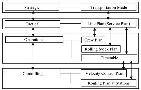
Figure 1.
Levels of the railway transportation planning work.
We can see that the operational plan and the controlling plan have a significant close connection, interacting with each other greatly. As we can see from Figure 1, a train timetable is essential to organize the operation of the trains. It is the base to design the crew plan and the rolling stock plan. It is also the constraint to deal with the train controlling problem, requiring that the train runs at an appropriate speed and through the stations according to a reasonable routing plan.
It is essential to study the integration of the operational plan and the controlling plan, avoiding the possibility of the invalidity of the operational plan. With the development of technology, train automatic driving has drawn researchers’ attention, which requires studying train re-scheduling and train control problem synthetically. We focus on this problem in this paper.
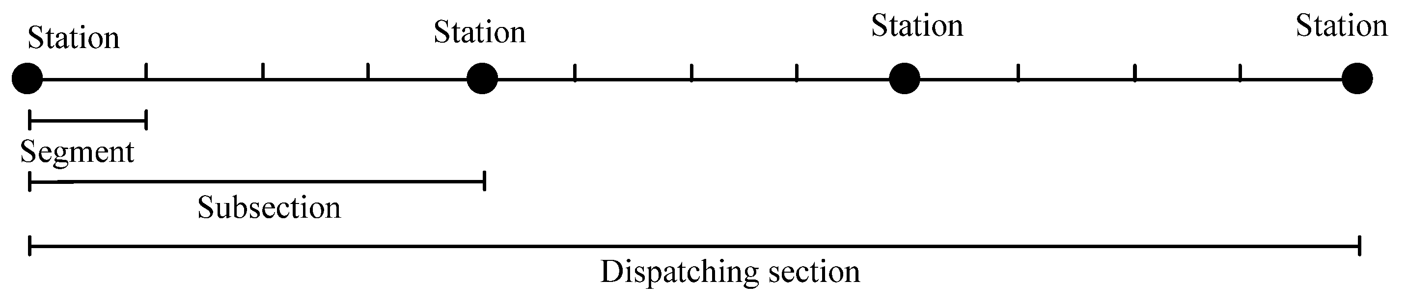
This paper involves several appellations of the railway sections. Here we give the definition. Dispatching section (or “section” only) refers to a section including some stations and segments, which is a unit for dispatching work. Segment refers to the subsection between two adjacent stations. A segment is divided into several segments because of the different longitudinal section and horizontal section by the turning points of the rail. We call the smallest unit of the section a segment, see Figure 2. We will study the train re-scheduling problem, determining the arrival and departure time of the trains at stations. We will also calculate the speed of the trains at the beginning and end of each section, controlling the movements of the trains, which belongs to the train control level.

Figure 2.
Description of several terms.
The main contribution of this paper is to present a novel approach to solve train re-scheduling and traction planning problem synthetically. It not only determines the arrival and departure time of the trains at stations, but also decides the traction plan of the trains. The approach presented in this paper can minimize the total delay time of the trains and assure the minimum energy consumption when the trains run between stations. We also utilize the quantum-inspired particle swarm optimization algorithm (QPSOA) to solve the proposed model. It is an innovation in the algorithm application. The approach in this paper can also provide supporting information for both the dispatchers and the train drivers to improve the on schedule rate and reduce the energy consumption.
The content of this paper is as follows. Section 2 reviews the related research on train re-scheduling and control problem. Section 3 builds an integrated model for train re-scheduling and control. Section 4 introduces QPSOA and gives the calculating steps for the model proposed in Section 3. Section 5 gives a computing case and analyzes the computing results. Section 6 draws the conclusion.
2. Literature Review
It is difficult to integrate the operational plan with the controlling plan. There are only a few publications on the integration of different levels of the problem. Carey proposed a model to help select the routes and platforms for the trains [1]. D’Ariano et al. focused on the reordering and rerouting problem, where reordering means to sequence the train movements and rerouting means to redesign the routes for the trains. They utilized a branch-and-bound algorithm and a local search algorithm to solve sequencing train movements problem and rerouting problem respectively [2]. Michaelis and Schöbel designed a heuristic method to solve the line planning, timetabling, and vehicle scheduling problem simultaneously [3]. Lee and Chen combined the train pathing and timetabling together and presented an optimization heuristic to solve real-sized instances [4]. Sun et al. proposed a multi-objective optimization model for train routing problem [5]. Groves et al. proposed a graph theoretic heuristic to select routes for a vehicle [6].
Most of the publications focus on problems belonging to only one of the levels. In recent years, many researchers have designed many train re-scheduling models. Schöbel proposed a model to improve the convenience of the passengers [7]. Tőrnquist and Persson presented a method to solve train re-scheduling problems on a railway network [8]. D’Ariano et al. built a job shop scheduling model to solve train re-scheduling problems [9]. Dündar and Şahin studied genetic algorithms for train re-scheduling problems [10]. Meng and Zhou constructed a single-track train re-scheduling model which optimized schedules for a relatively long rolling horizon. We put forward the definition of train timetable stability and optimized the train timetable based on the definition and also proposed an improved fuzzy linear programming model to solve train re-scheduling problems [11]. Chen et al. designed a model to generate a train timetable, considering the capacity of a railway section [12]. Chen et al. developed a departure time domain, considering capacities of arrival-departure tracks [13]. Yang et al. constructed an approach to rescheduling the metro trains, taking the energy consumption into consideration [14]. Wen et al. designed a cause-specific approach to identify the delay causalities and solve train re-scheduling problems [15]. Chang et al. proposed an integrated scheduling model, which integrated the scheduling of rail-mounted gantry cranes, inner trucks, and yard cranes [16]. Chen and Sun developed a multistate-based model to design travel time schedule for fixed transit route and designed a Monte Carlo simulation-based genetic algorithm procedure to obtain the optimal slack time [17]. Corman designed a model to resolve the re-scheduling and routing problem comprehensively [18]. Zhu and Goverde dealt with train re-scheduling problems, taking it for granted that the rails between stations are not available for several hours [19]. Zinder et al. designed a novel model to handle the eventuality of one track of a double-track railway becoming unavailable [20].
There are also some publications on the real-time re-scheduling problem. Mazzarello and Ottaviani described an architecture of a real-time traffic management system that had been successfully used [21]. Rodriguez combined the train pathing and reordering problem [22]. Cacchiani et al. studied the train re-scheduling where there were both passenger trains and freight trains [23]. Acuna-Agost et al. built a mixed-integer programming model to solve the real-time re-scheduling problem [24,25]. Krasemann designed a depth-first search algorithm to solve the train real-time re-scheduling problem [26]. Almodóvar and García-Ródenas proposed an on-line optimization model for train re-scheduling problem [27]. Dalapati et al. presented novel agent-based solution approach to handle the real-time collision in train re-scheduling work [28]. Altazinab et al. presented a simulation method for re-scheduling problem [29]. Huang et al. designed mixed integer programming models to solve the train re-scheduling problem [30].
In addition, the train control problem has been paid much attention in recent years. Dong et al. introduced railway traffic automatic control systems in Chinese high-speed train system in detail and proposed a numerical modeling of high-speed trains. They also simulated the train movements and analyzed the simulation results [31]. Song et al. presented a dynamic model that reflected resistance in train tracking control to solve the train control problem [32]. Zhou and Wang proposed the generalized and hierarchical framework of model predictive control for the railway system including macroscopic, macroscopic, and microscopic levels [33]. Yang et al. constructed a model to find optimal train movements under the consideration of operational interactions [34]. Wang et al. proposed a pseudo spectral method, a state-of-the-art method for optimal control problems [35]. Faieghi et al. redefined the robust adaptive cruise controller and analyzed the rigorous stability [36]. Li et al. investigated the robust cruise control scheduling of high-speed train based on sampled data [37]. Su et al. proposed a cooperative train control model to minimize the practical energy consumption [38]. Bersani et al. addressed the time-honored problem of scheduling trains on a single track, in the light of related results in robust team decision theory [39]. Li et al. investigated the coordinated cruise control strategy for multiple high-speed trains’ movement [40].
We can see that the majority of publications above focus on one of the problems, either on the train re-scheduling problem, or the train control problem. Only a few of them combine both the problems together. Two papers study problems similar to those which we study. Xu et al. built a train re-scheduling model integrating speed design [41]. There are some differences between their model and ours. Firstly, the type of the models is different. Their model is a MILP (mixed integer linear programming) model and ours is a non-linear model. Secondly, the goal of the model is to minimize the secondary delay of traffic running, while the goal of our model is to minimize the difference of the re-scheduled timetable and the planned timetable. Thirdly, speed in their model is considered in the constraints design work, while we study the train control mode (when to alternate the train mode) to reduce the energy consumption. Lastly, they utilized the commercial software to solve the model and we design a heuristic algorithm to solve the model. We have published another paper which combined the train re-scheduling problem and track assignment problem, which not only determines the arrival and departure time of the trains at the stations, but also decides which tracks the trains should occupy in the stations. It is different from the problem presented in this paper, which tries to give the arrival and departure time, together with the operation modes in the railway sections.
3. Integrated Model for Re-Scheduling and Control
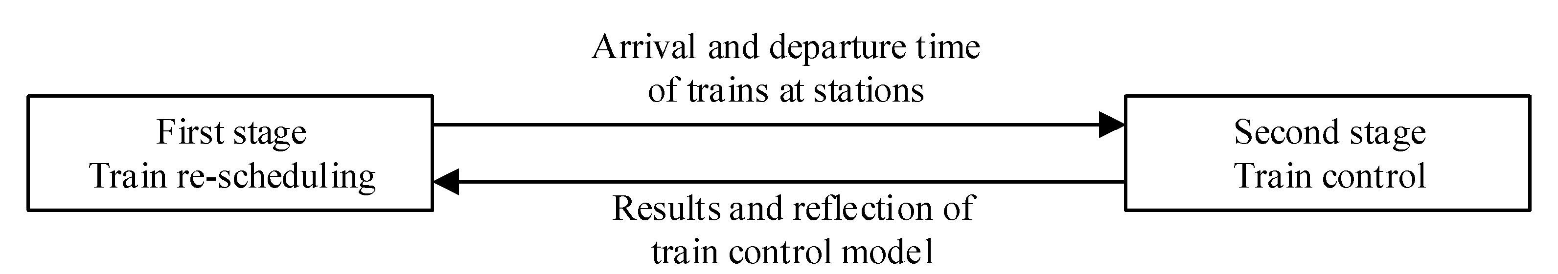
It is obvious that two problems must be solved when dispatching the trains on the railways, which are closely tied to each other. Re-scheduling is to adjust the order of the trains to run through the stations and the arrival and departure time of the trains. The task of control is to adjust the speed of the trains to arrive at the stations in time. Therefore, it can be concluded that the results of train re-scheduling problem (arrival and departure time of the trains at stations) are the base and constraints of the train control problem, requiring the arrival and departure time of the trains. Based on the characteristics analyzed above, we designed a bi-stage model to solve the train re-scheduling and control problem, see Figure 3.

Figure 3.
Relation between the train re-scheduling problem and train control problem.
Statement of the first stage model:
Based on the planned timetable, we must reduce the total time of delay when disturbances occur, considering the speed limit, the intervals between trains, etc.
The input data of the train re-scheduling problem are
- Intervals of the trains,
- Minimum running time at each segment,
- Minimum dwelling time at all the stations of each train.
The output data of the problem are the arrival and departure times of the trains at all stations.
Statement of the second stage model:
Under the constraints of the operation time of the trains at stations, we must identify the speed and speed changes when running on all the segments. The input data of the train control problem are the arrival and departure time of the trains at stations. The output data is the speed of the trains when running on the segments, and the change in speed when the condition of the rail varies, including the flat and vertical section.
3.1. Variables and Parameters of the Model
The related variables and parameters are listed in Table 1.

Table 1.
Variables and parameters of the model.
3.2. First Stage-Train Re-Scheduling Problem
3.2.1. Objective of Train Re-Scheduling Model
Generally, the aim of train re-scheduling is to recover the status of all trains running as per the original train diagram. There are several indices to measure the recovering degree, the on schedule rate, the delay rate, and the difference between the re-scheduled and original timetables. We have defined the gap based on arrival and departure time of the trains in a previous paper [13]. In this paper, we also use the definition in Reference [13], shown as Equation (1).
It describes the gap between the re-scheduled timetable and the original timetable, calculating the total delay time if the trains run as the re-scheduled timetable. Since the re-scheduled arrival time of a train at a station in the re-scheduled timetable may be earlier than in the original timetable, we use the max function to take the larger value from , and 0, avoiding the adverse effect of early arrival of a certain train.
3.2.2. Constraints for Train Re-Scheduling Model
When trains are running in the sections, arriving at stations and departing from stations, we must assure the safety of all the trains. The intervals are designed to keep the safe distance between trains, constructed with the time needed to pass a certain number of subsection, the time needed to do the arrival action, the time needed to do the departure action, the time needed for the divers to accept the signals and make corresponding actions, and the time needed for extra protection. The intervals are already calculated and have come into the operating rules.
The operation interval constraints to assure the arrival and departure safety are shown as Equations (2) and (3).
In addition, some of the stations cannot send a train and receive a train at the same time. The constraint is described in Equation (4).
Equation (5) requires that the re-scheduled running time is longer than the allowed minimal running time.
Equation (6) requires the re-scheduled dwelling time is longer than the allowed minimal dwelling time.
Passenger trains must not depart before the time as it is planned on the original timetable.
3.2.3. Mathematical Model
The mathematical model of this problem is constructed as follows:
3.3. Second Stage-Train Control Problem
The second stage of the model is to design the speeds and the speed changes of the trains when the train runs on the rail. The goal is to determine the traction plan and calculate the speed of all the trains at the beginning and end of each segment, matching the arrival time of the trains at the next station. Therefore, we can see that there are many plans which must be manipulated to make the trains arrive at the stations in time, see Figure 4.
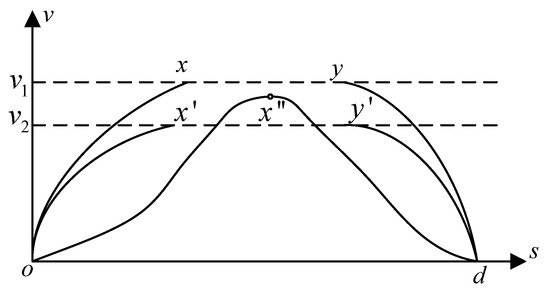
Figure 4.
Description of the train control plan.
There are three control plans shown in Figure 4. o is the beginning of the segment and the d is the end of the segment. The first one is to accelerate the train to a high-speed (o-x), and then run at the speed of (x-y), and then it causes the train to brake (y-d). The second is similar to the first plan. The train accelerates, runs at a constant speed , then it brakes. The third one is to accelerate the train to a speed, then it slows the train to a coasting drift (o-x″-d). Three control plans all cause the train to reach the end of the segment. The difference is that the goal of the first plan is to save time and that of the third plan is to save tractive force energy. Which one is the best? Generally, the third one is the best from the perspective of saving energy if it meets the arrival time of the trains at stations.
Therefore, in this paper we take the consumed energy as the optimizing goal.
is the consumed energy of train i, at segment j.
The processes that consume the energy are accelerating process, the braking process, and the process of running at a constant speed.
When the train accelerates,
So,
Then the tractive force is:
When the train runs at a constant speed, the tractive force must conquer the friction force between the train and the track. So,
When the train brakes,
The tractive force can be calculated then. How to evaluate the consumed energy? We take the “work” that the tractive force does to evaluate. We describe as follows.
Then the second stage-train control model is described as follows.
Here, we need to derive the formulas to calculate the consumed energy, the running time of a train in each segment, and the velocity at the end of each segment. Since the different types of EMUs (electric multiple units) have different basic resistance formula, we need to select the type of EMU to complete the derivation. The computing case in Section 5 is based on CRH3 (China Railway High-Speed-Vehicle Type 3). Therefore, we did the derivation work based on the resistance formula of CRH3.
In Equation (21), the measurement unit of is km/h, so it equals to:
where the measurement unit of is m/s.
In Equation (22), the measurement unit of is m/s. To unify the all the measurement units to a standard system, Equation (22) can be changed into Equation (23).
where the measurement unit of is m/s and the measurement unit of is N/KG.
Thus, if a train accelerates at a certain acceleration, the consumed energy in the acceleration process ( in Equation (19)) is:
We take it for granted that a train does not consume energy when it coasts or brakes.
In addition, the consumed energy in the process of running at a constant speed can also be calculated with Equation (24). Therefore, we get the equation for calculating the consumed energy.
The destination is to give a control plan for each segment to assure the running operation time of a train in a whole section and keep the consumed energy to be minimal. The control plan will determine the operation mode, thus determining the running time and the velocity at the end of a segment.
4. Quantum-Inspired PSO for the Integrated Model
4.1. Particle Swarm Optimization Algorithm
Quantum Particle Optimization (PSO) algorithm is a PSO which uses quantum inspired evolutionary algorithm theory. The positions of the particles are defined with the quantum bits. The PSO algorithm was first introduced by Eberhart and Kennedy [42]. It has been proved that PSO is an effective optimization algorithm in recent years. In this paper, we improved the algorithm with quantum inspired thought.
4.2. Quantum Particle Swarm Optimization Algorithm
The quantum particle swarm algorithm is a new version of particle swarm optimization algorithm. Compared with the typical particle swarm optimization algorithm, the most important difference is the description form of the particle positions and the velocity equation. The description of the positions and velocity uses the quantum concept.
The original positions of the particles are described with the probability amplitude of the quantum.
where , is a random number, , , , i is the number of the particles, and j is the dimensionality of a particle.
Then the most important work is to change the particle positions into real numbers, which can describe the solution of the engineering problems. Set to be the lower boundary of jth dimension of a particle and to be the upper boundary of jth dimension of a particle. Then is the value range.
Set to be the jth quantum position. The position of the solution can be defined as follows.
We can see that the solution is defined with the key element . We can adjust the solution by change the value of .
Set to be the current best solution and to be the global best solution of the optimization problem.
Then the change of argument of particle can be represented as:
where
The quantum rotation gate is:
Then the operation of the change of argument of the quantum is:
The new positions of particle are as follows:
Thus, the change of the particle position is completed. We can calculate fitness value of the optimization model to judge whether the position is better. Then we decide how to adjust the velocity and position of the particles.
4.3. QPSO for Resolving Train Re-Scheduling and Control Problem
The QPSO algorithm for train re-scheduling problem is as follows.
- Step 1: To initiate all the original solution and parameters of the model;
- Step 2: To calculate the fitness value of the model according to Equation (1) when solving train re-scheduling problem (Equation (19) when solving train control problem);
- Step 3: To calculate the change of argument of the particles according to Equation (30);
- Step 4: To calculate the positions of the particles according to Equation (35) and Equation (36);
- Step 5: To calculate the fitness value of the model according to Equation (1) when solving train re-scheduling problem (Equation (19) when solving train control problem);
- Step 6: To select the optimal local and global particle from the two swarms;
- Step 7: To check if the computational accuracy satisfies the requirements. If yes, stop; otherwise, go to step 3.
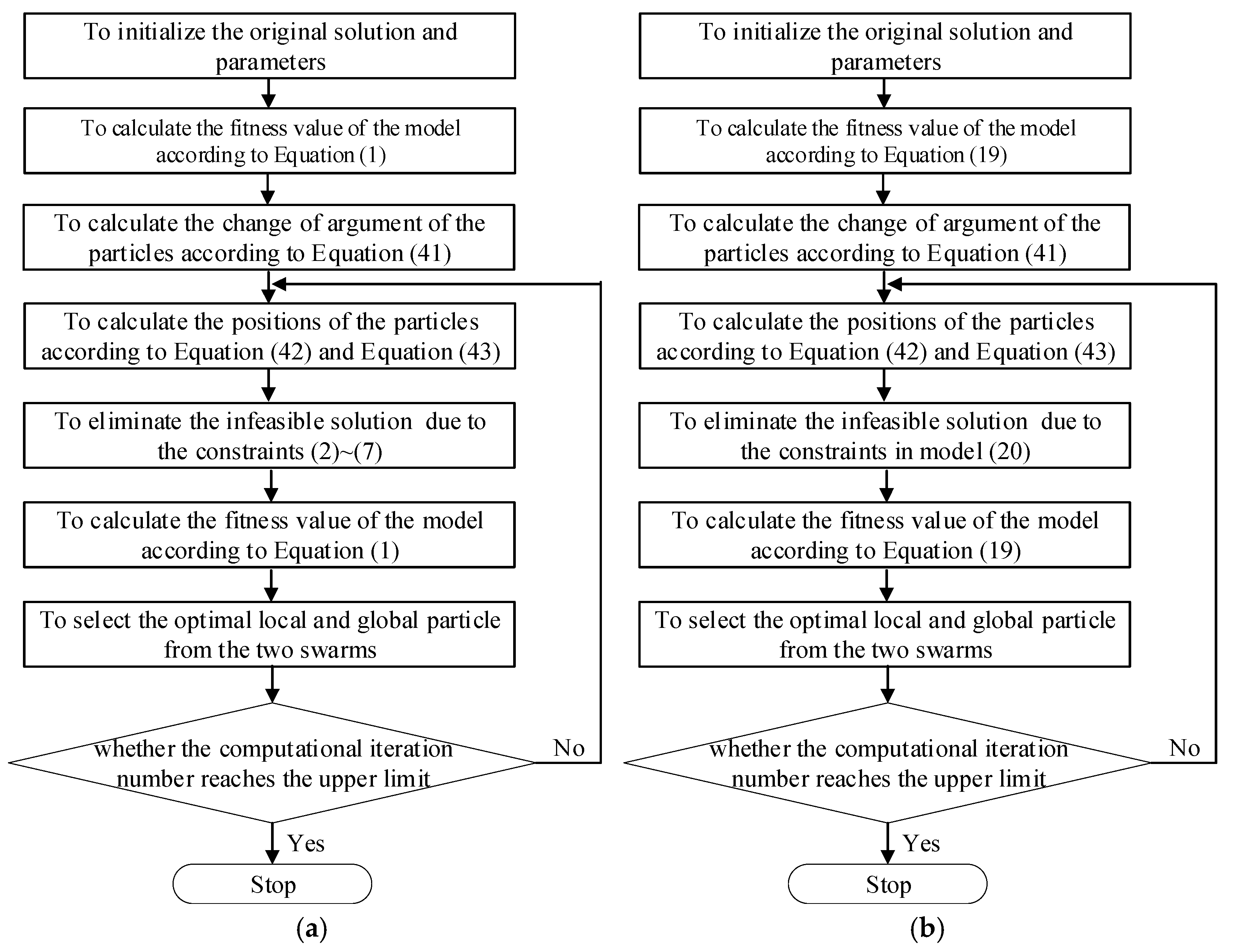
The flowchart of the algorithm for the train re-scheduling stage is shown as Figure 5a and that for the train control problem is shown in Figure 5b.
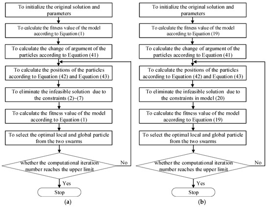
Figure 5.
Flowcharts of the algorithms for the two stages of the model. (a) Algorithm flowchart for train re-scheduling problem; (b) Algorithm flowchart for train control problem.
5. Computation Case and Results Analysis
5.1. Basic Data of the Computing Case
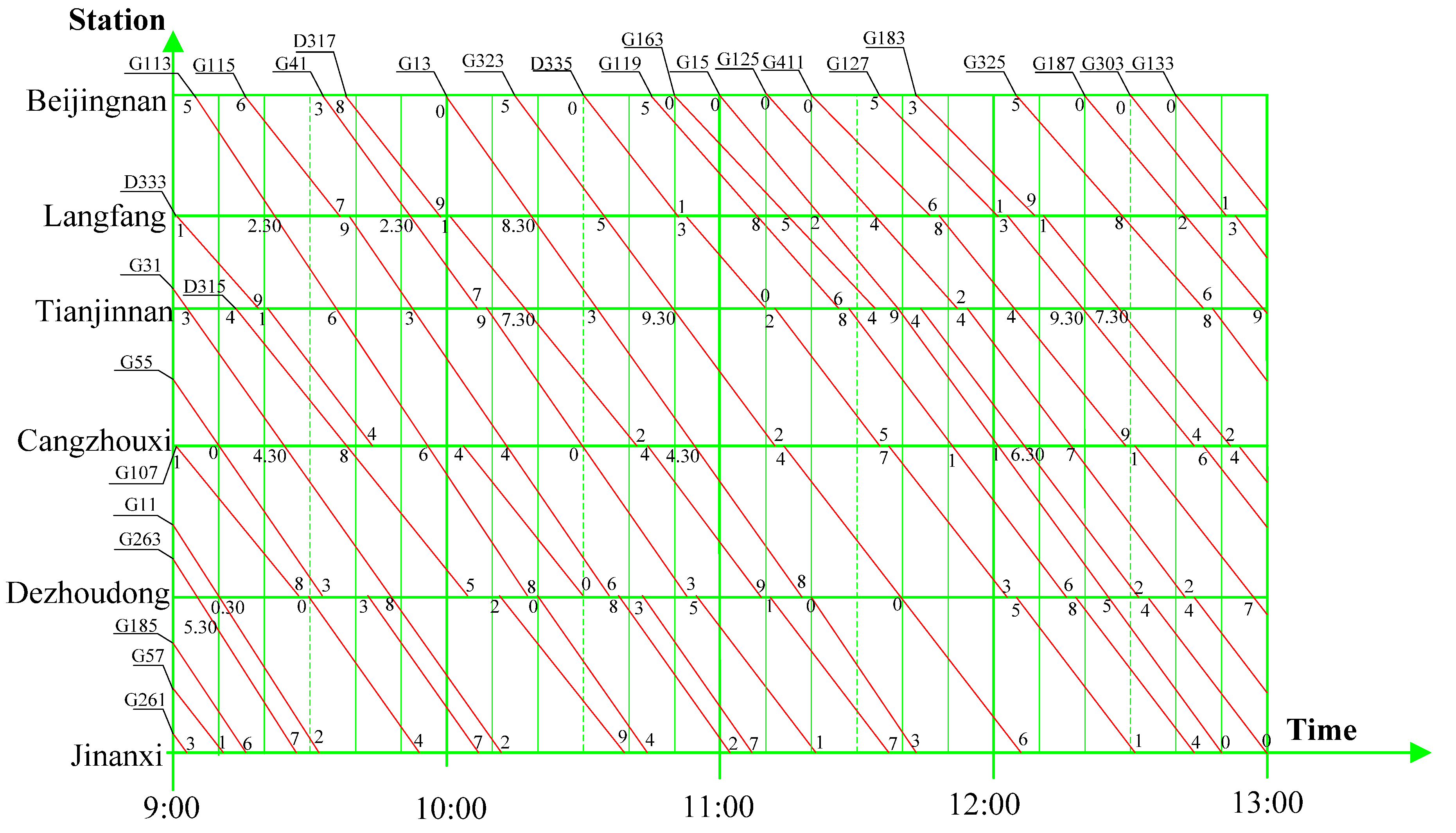
We did the data experiment based on the real operation data of Beijing-Shanghai high-speed railway. The timetable is between Beijingnan and Jinanxi station from 9:00 to 13:00. There are six stations in the studied section: Beijingnan, Langfang, Tianjin, Canzhouxi, Dezhoudong, and Jinanxi. The number of related trains is 28. There are two types of trains in this case, the G type trains and D type trains. G and D are the initials of two types of Chinese high-speed trains. D type trains have a maximum speed of under 250 km/h and a top speed of 200–250 km/h. The speed of G type trains is no less than 250 km/h. The top speed is 300–350 km/h.
The original train diagram is shown in Figure 6 and the arrival and departure time of the trains at the stations are listed in Table 2.
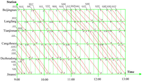
Figure 6.
Original train diagram between Beijingnan and Jinanxi (south-going direction) from 9:00 to 13:00.
Table 2.
Original train timetable between Beijingnan and Jinanxi (south-going direction) from 9:00 to 13:00.
The minimal running time of the trains is shown in Table 3.
Table 3.
Minimal running time of the trains in all the segments.
In addition, there has been a stops plan, to decide which trains to stop at which stations. When we re-schedule the trains, we cannot change the stops plan. The minimum dwelling time at a station is 2 min. Some of the trains may dwell 10 min to wait for a backward train to overpass it. For example, G163 stays at Tianjinnan station to wait for G15 to overpass it.
The minimum interval between two departures from a same station or two arrivals at a same station is 5 min. In addition, the current allowed maximal speed is 300 km/h on Beijing-Shanghai high-speed railway.
We instantiated the model, setting the parameters firstly. The arrival time and the departure time, as well as the accelerations of the trains, and the consumed time were the decision variables in the model. The arrival and departure time were changed into the seconds number from 0:00. The initial solution can be built with the numbers. We chose 28 trains and 6 stations in this computing case and there were 21 segments in the railway section due to Figure 6.
Thus, the total number of units in the initial solution vector which stands for the arrival time and departure time is , because it is not necessary to decide the arrival time at Beijingnan and departure time at Jinanxi of the trains. To do the train control data experiment, we find the track profile of the segment from Beijingnan to Langfang, shown in Figure 7. We only calculate the train control plan in the section of Beijingna to Langfang in the south-going direction. Therefore, the number of the elements in the solution vector which stands for the accelerations is , and that of the elements in the solution vector which stands for the consumed time is . Therefore, the total number of the units in the solution vector is .

Figure 7.
Track profile of segment from Beijingnan to Langfang.( Note: Vertical line is the boundary between the segments, the number above the horizontal line or the diagonal is the inclination angle of the segment ((Measurement Unit: degree) and the number under the horizontal line or the diagonal is the distance of the segment (Measurement Unit: m)).
We set the iteration time of the computing to be 1000. The parameters are both set to be 2 in the optimization algorithm. The particle group size is set to be 40.
The type of the EMU is CRH3. CRH3 has a starting acceleration of 0.5 m/s2. Average acceleration is 0.38 m/s2. The maximal deceleration is −1 m/s2. The weight of CRH3 is 380,000 Kg.
There are two fitness functions in this model. The fitness function of train re-scheduling problem (first stage) is as Equation (1), which can be described as
The fitness function of train control is as Equation (19), which is:
Thus, the task is to calculate a train re-scheduling plan to dispatch the trains. We need to calculate a train control plan to guide the train driver to manipulate the train in the section from Beijingnan to Langfang.
5.2. Computation Results and Discussion
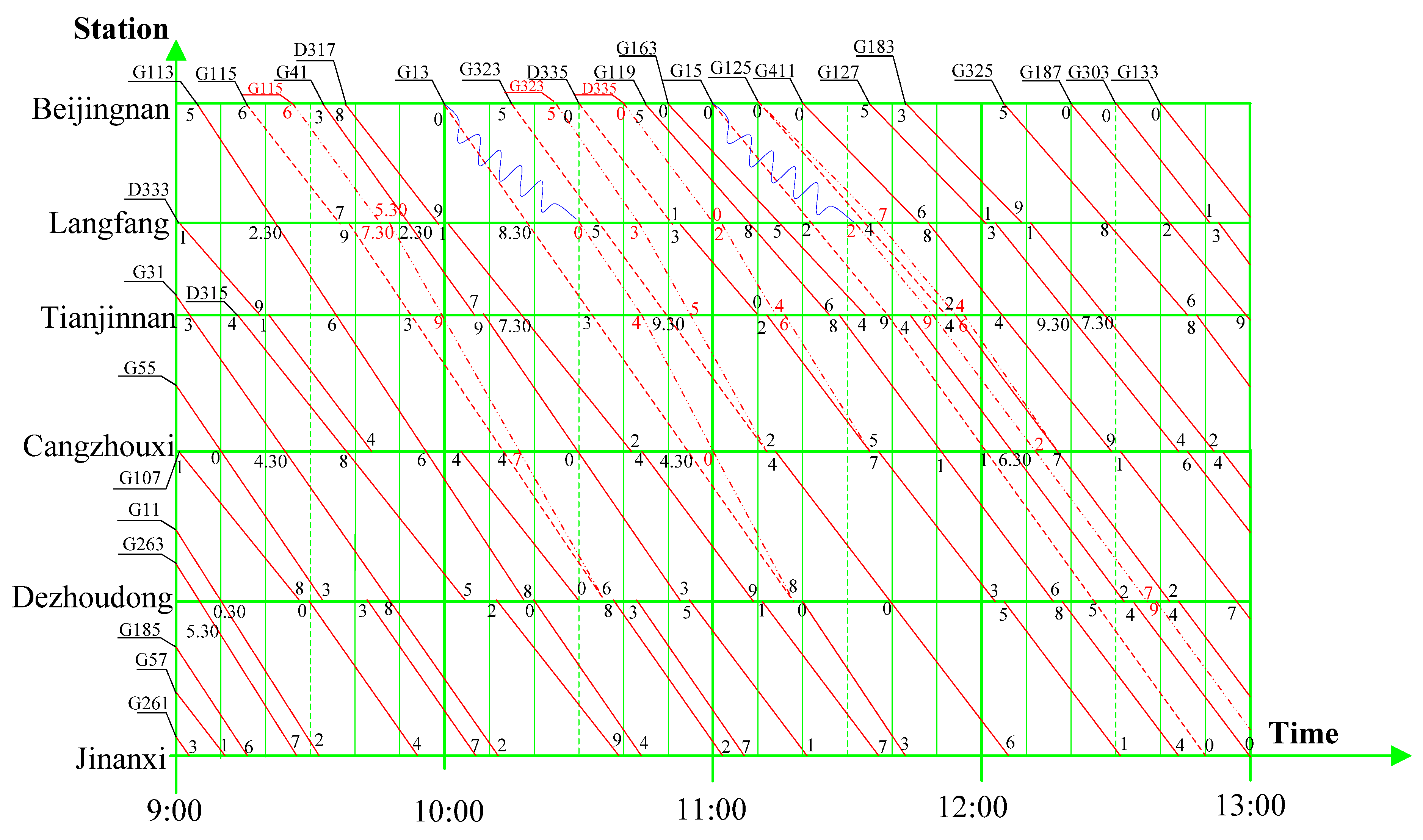
We took it for granted that four trains were delayed in the computing case. G115 and G323 were 10 min late at the origin station, Beijingnan, and EMU setup work was disturbed. G13 and G15 were delayed 10 min when arriving at Langfang station.
According to the model and the algorithm, we calculated a train re-scheduling plan, shown in Figure 8. The detailed timetable is shown in Table 4.
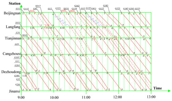
Figure 8.
Re-scheduled train diagram between Beijingnan and Jinanxi (south-going direction) from 9:00 to 13:00.
Table 4.
Part of Re-scheduled train timetable between Beijingnan and Jinanxi (south-going direction) from 9:00 to 13:00.
According to the calculation result, G115, G13, and D335 recovered the status that it ran according to the original timetable. The total delayed time of Train G115 is 45 min. The relative number of G13 is 56 min and relative number of D335 is 36 min. G15 did not recover to run according to the original timetable, for the following trains have the same degree as G15 and the dispatching rule is to ensure the operation plans of the trains are delayed as little as possible. The total delayed time is 86 min. Furthermore, G125 is affected by G15, as the minimum interval between two arrivals is 5 min. The total delay time of G125 is 10 min. The total delay time of all the trains at all the stations is 270 min.
Due to the operation rule by Meng in the previous publications, the train will be scheduled to run as fast as possible, which means that it will be scheduled to finish the running within the minimum running time [43,44,45]. However, we can find that G115 did not run as fast as possible, for the minimum running time is 18 min, while the re-scheduled running time is 19.5 min in this computing case. That is because we not only give the train re-scheduling plan as the previous publication, but also consider the train control plan, which aims to save energy. The detailed control plan is listed below.
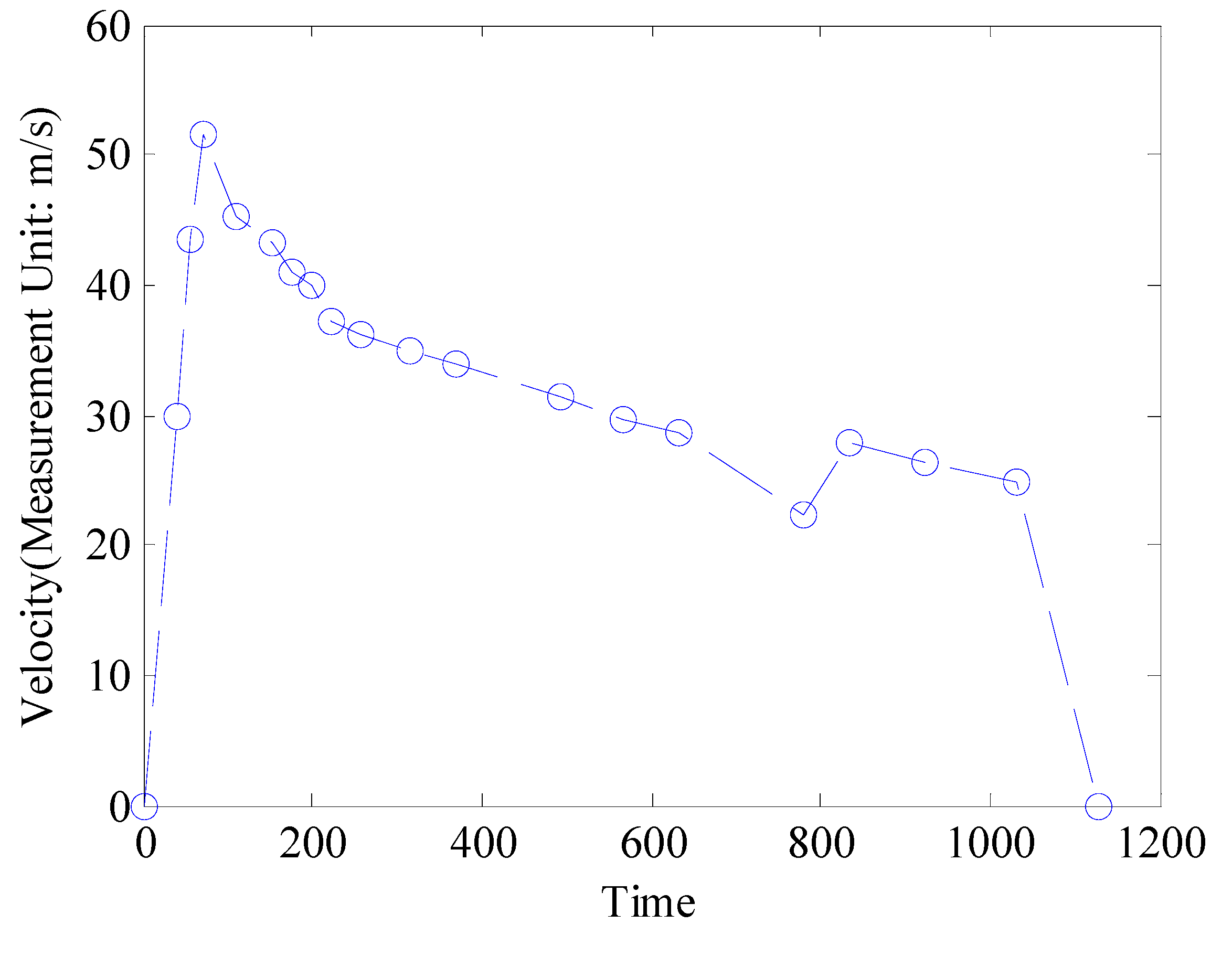
From Table 5, we can see that we need to accelerate Train G115 in four segments. The calculating result requires the train to accelerate at the first three segments. Then it coasts in the following 12 segments and the velocity decreases from 51.478 m/s to 28.728 m/s. It accelerates at the 16th segment, with the speed reaching to 27.832 m/s. After that it coasts for another segment. In the last segment, it brakes at the deceleration of −0.26 m/s2. We can see that the curve has a downward trend and the slope is declining. This is because the basic resistance is related to the velocity. With the decreasing of the train, the resistance is decreases, and the deceleration is diminishing. Then the velocity decreases. This is a loop process.
Table 5.
Train control plan for G115 in section between Beijingnan and Langfang in the south-going direction.
The total running time is 1169.527 s. It satisfies the requirement that the time for trains to operate from Beijingnan to Langfang is 1170 s (19.5 min).
We can see from Figure 9 that when the train is near Langfang, the speed is low. This is because a train with a low speed is easy to control. It not only benefits for the safety of train operation, but also for the saving of traction energy. The energy consumed in the four acceleration processes are , , , and joule separately.
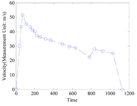
Figure 9.
Control plan of G115 from Beijingnan to Langfang.
The maximal speed in the whole process is 51.478 m/s, which equals to 185.32 km/h. The speed is much lower than the allowed maximal speed. However, we find that the total consumed time from Beijingnan to Langfang is less than 19.5 min. This reflects the fact that the timetable has reserved a somewhat large space to re-schedule the trains.
Can we speed up the trains at the first several segments to faster than 51.478 m/s and brake at the end of the section? It is possible, but it is not necessary. If we do so, more energy will be wasted. In addition, the maximal deceleration is −1.0 m/s2. If the velocity is too high, it is possible that the train would be unable to stop at Langfang as planned. The control plan can ensure the train arrives at Langfang on time, and it is an optimal control plan to minimize the consumed energy.
6. Conclusions
An integrated model for train re-scheduling and control is proposed. The model can be divided into two stages. The first stage is to re-schedule the trains when the trains are disturbed, deciding the arrival and departure time of the trains at the stations. Thus, the running time of each train can be calculated to set constraints for the train control problem. A train control approach is proposed, which is the second stage of the integrated model. Since it is quite important to have the perfect control plan, we designed the model to decide which manipulation mode should be taken in each segment. We derived the formula to calculate the energy, the running time, and the distance and provided a method to calculate the optimal control plan to minimize the consumed energy in the premise of meeting the requirement of the running time. The integrated model can give the train re-scheduling plan and the train control plan synchronously. Train re-scheduling plan can provide supporting information for the train dispatchers and the train control plan is helpful for the train drivers. Therefore, it can be seen as a theory base for self-driving technology. It can also avoid the risk that the train timetable cannot be executed, for there may be no feasible traction plan for the trains, although the timetable is generated.
In future works we will continue studying the train control problem (the second stage problem in this paper), generating the traction plan for all of the related trains. We will try to merge the train re-scheduling and train control (routing in the station and traction planning) problems to further support the train dispatching work.
Author Contributions
Investigation, X.M.; project administration, Y.W.; writing—original draft, Y.W.; writing—review and editing, L.L. (Li Lin); data curation, L.L. (Lei Li); validation, L.J. All authors have read and agreed to the published version of the manuscript.
Funding
This work is supported by Key Laboratory of Urban Rail Transit Intelligent Operation and Maintenance Technology & Equipment of Zhejiang Province, “Double-First Class” Major Research Programs, Educational Department of Gansu Province (No. GSSYLXM-04), the National Natural Science Foundation of China (Grant No. 71861022), the Young Teachers Program of Lanzhou Jiaotong University (Grant: 2019039), the Foundation of A Hundred Young Talents Training Program of Lanzhou Jiaotong University (Grant No. 1520220210), and the State Key Laboratory of Rail Traffic Control and Safety, Beijing Jiaotong University.
Institutional Review Board Statement
Not applicable.
Informed Consent Statement
Not applicable.
Data Availability Statement
All data, models, and code generated or used during the study appear in the submitted article.
Acknowledgments
The authors wish to thank the anonymous referees and the editor for their comments and suggestions.
Conflicts of Interest
The authors declare no conflict of interest.
References
- Carey, M. A model and strategy for train pathing with choice of lines, platforms and routes. Transp. Res. B Methodol. 1994, 28, 333–353. [Google Scholar] [CrossRef]
- D’Ariano, A.; Corman, F.; Pacciarelli, D.; Pranzo, M. Reordering and local rerouting strategies to manage train traffic in real time. Transp. Sci. 2008, 42, 405–419. [Google Scholar] [CrossRef]
- Michaelis, M.; Schöbel, A. Integrating line planning, timetabling, and vehicle scheduling: A customer-oriented heuristic. J. Public Transp. 2009, 1, 211–232. [Google Scholar] [CrossRef] [Green Version]
- Lee, Y.; Chen, C.Y. A heuristic for the train pathing and timetabling problem. Transp. Res. B Methodol. 2009, 43, 837–851. [Google Scholar] [CrossRef]
- Sun, Y.; Cao, C.; Wu, C. Multi-objective optimization of train routing problem combined with train scheduling on a high-speed railway network. Transp. Res. C Emerg. Technol. 2014, 44, 1–20. [Google Scholar] [CrossRef]
- Groves, G.; Roux, L.J.; Vuuren, J.H.V. Network service scheduling and routing. Int. Trans. Oper. Res. 2004, 11, 613–643. [Google Scholar] [CrossRef]
- Schöbel, A. A model for the delay management problem based on mixed-integer-programming. Electron. Notes Theor. Comput. Sci. 2001, 50, 1–10. [Google Scholar] [CrossRef] [Green Version]
- Tőrnquist, J.; Persson, J.A. N-tracked railway traffic re-scheduling during disturbances. Transp. Res. B Methodol. 2007, 41, 342–362. [Google Scholar] [CrossRef]
- D’Ariano, A.; Pacciarelli, D.; Pranzo, M. A branch and bound algorithm for scheduling trains in a railway network. Eur. J. Oper. Res. 2007, 183, 643–657. [Google Scholar] [CrossRef]
- Dundar, S.; Şahin, I. Train re-scheduling with genetic algorithms and artificial neural networks for single-track railways. Transp. Res. C Emerg. Technol. 2013, 27, 1–15. [Google Scholar] [CrossRef]
- Meng, L.; Zhou, X. Robust single-track train dispatching model under a dynamic and stochastic environment: A scenario-based rolling horizon solution approach. Transp. Res. B Methodol. 2011, 45, 1080–1102. [Google Scholar] [CrossRef]
- Chen, D.; Ni, S.; Xu, C.; Jiang, X. Optimizing the draft passenger train timetable based on node importance in a railway network. Transp. Lett. 2019, 11, 20–32. [Google Scholar] [CrossRef]
- Chen, D.; Ni, S.; Lv, H.; Li, H. Genetic algorithm based on conflict detecting for solving departure time domains of passenger trains. Transp. Lett. 2015, 7, 181–187. [Google Scholar] [CrossRef]
- Yang, X.; Chen, A.; Wu, J.; Gao, Z.; Tang, T. An energy-efficient rescheduling approach under delay perturbations for metro systems. Transp. B Trans. Dyn. 2018, 7, 386–400. [Google Scholar] [CrossRef]
- Wen, C.; Li, Z.; Huang, P.; Lessan, J.; Fu, L.; Jiang, C. Cause-specific investigation of primary delays of Wuhan–Guangzhou HSR. Transp. Lett. 2019, 12, 451–464. [Google Scholar] [CrossRef]
- Chang, Y.; Zhu, X.; Yan, B.; Wang, L. Integrated scheduling of handling operations in railway container terminals. Transp. Lett. 2019, 11, 402–412. [Google Scholar] [CrossRef]
- Chen, S.; Sun, D. A multistate-based travel time schedule model for fixed transit route. Transp. Lett. 2019, 11, 33–42. [Google Scholar] [CrossRef]
- Corman, F. Interactions and equilibrium between rescheduling train traffic and routing passengers in microscopic delay management: A game theoretical study. Transp. Sci. 2020, 54, 758–822. [Google Scholar] [CrossRef]
- Zhu, Y.; Goverde, R.M.P. Dynamic and robust timetable rescheduling for uncertain railway disruptions. J. Rail Transp. Plan. Manag. 2020, 15, 100196. [Google Scholar] [CrossRef]
- Zinder, Y.; Lazarev, A.; Musatova, E. Rescheduling traffic on a partially blocked segment of railway with a siding. Automat. Remote Control 2020, 81, 955–966. [Google Scholar] [CrossRef]
- Mazzarello, M.; Ottaviani, E. A traffic management system for real-time traffic optimization in railways. Transp. Res. B Methodol. 2007, 41, 246–274. [Google Scholar] [CrossRef]
- Rodriguez, J. Constraint programming model for real-time trains scheduling at junctions. Transp. Res. B Methodol. 2007, 41, 231–245. [Google Scholar] [CrossRef]
- Cacchiani, V.; Caprara, A.; Toth, P. Scheduling extra freight trains on railway networks. Transp. Res. B Methodol. 2010, 44, 215–231. [Google Scholar] [CrossRef]
- Acuna-Agost, R.; Michelon, P.; Feillet, D.; Gueye, S. A MIP-based local search method for the railway re-scheduling problem. Networks 2011, 57, 69–86. [Google Scholar] [CrossRef]
- Acuna-Agost, R.; Michelon, P.; Feillet, D.; Gueye, S. SAPI: Statical analysis of propagation of incidents. A new approach for re-scheduling trains after disruptions. Eur. J. Oper. Res. 2011, 215, 227–243. [Google Scholar] [CrossRef]
- Krasemann, J.T. Design of an effective algorithm for fast response to the re-scheduling of railway traffic during disturbances. Transp. Res. C Emerg. Technol. 2012, 20, 62–78. [Google Scholar] [CrossRef]
- Almodóvar, M.; García-Ródenas, R. On-line reschedule optimization for passenger railways in case of emergencies. Comput. Oper. Res. 2013, 40, 725–736. [Google Scholar] [CrossRef]
- Dalapati, P.; Padhy, A.; Mishra, B.; Dutta, A.; Bhattacharya, S. Real-time collision handling in railway transport network: An agent-based modeling and simulation approach. Transp. Lett. 2019, 11, 458–468. [Google Scholar] [CrossRef]
- Altazinab, E.; Dauzère-Pérèsbc, S.; Ramond, F.; Trefond, S. A multi-objective optimization-simulation approach for real time rescheduling in dense railway systems. Eur. J. Oper. Res. 2020, 286, 662–672. [Google Scholar] [CrossRef]
- Huang, Y.; Mannino, C.; Yang, L.; Tang, T. Coupling time-indexed and big-M formulations for real-time train scheduling during metro service disruptions. Transp. Res. B Methodol. 2020, 133, 38–61. [Google Scholar] [CrossRef]
- Dong, H.R.; Ning, B.; Cai, B.; Hou, Z. Automatic train control system development and simulation for high-speed railways. IEEE Circuits Syst. Mag. 2010, 10, 6–18. [Google Scholar] [CrossRef]
- Song, Q.; Song, Y.D.; Tang, T.; Ning, B. Computationally inexpensive tracking control of high-speed trains with traction/braking saturation. IEEE Intell. Transp. Syst. 2011, 12, 1116–1125. [Google Scholar] [CrossRef]
- Zhou, Y.H.; Wang, Y.P. Coordinated control among high-speed trains based on model predictive control. Key Eng. Mater. 2011, 467, 2143–2148. [Google Scholar] [CrossRef]
- Yang, L.X.; Li, K.P.; Gao, Z.Y.; Li, X. Optimizing trains movement on a railway network. Omega 2012, 40, 619–633. [Google Scholar] [CrossRef]
- Wang, Y.H.; Schutter, B.D.; van den Boom, T.J.J.; Ning, B. Optimal trajectory planning for trains—A pseudospectral method and a mixed integer linear programming approach. Transp. Res. C Emerg. Technol. 2013, 29, 97–144. [Google Scholar] [CrossRef]
- Faieghi, M.; Jalali, A.; Mashhadi, S.K.M. Robust adaptive cruise control of high-speed trains. ISA Trans. 2014, 53, 533–541. [Google Scholar] [CrossRef]
- Li, S.K.; Yang, L.X.; Li, K.P.; Gao, Z. Robust sampled-data cruise control scheduling of high-speed train. Transp. Res. Emerg. Technol. 2014, 46, 274–283. [Google Scholar] [CrossRef]
- Su, S.; Tang, T.; Roberts, C. A cooperative train control model for energy saving. IEEE Trans. Intell. Transp. 2015, 16, 622–631. [Google Scholar] [CrossRef]
- Bersani, C.; Qiu, A.; Sacile, R.; Sallak, M.; Schon, W. Rapid, robust, distributed evaluation and control of train scheduling on a single line track. Control Eng. Pract. 2015, 35, 12–21. [Google Scholar] [CrossRef]
- Li, S.; Yang, L.; Gao, Z. Coordinated cruise control for high-speed train movements based on a multi-agent model. Transp. Res. C Emerg. Technol. 2015, 56, 281–292. [Google Scholar] [CrossRef]
- Xu, P.; Corman, F.; Peng, Q.; Luan, X. A train rescheduling model integrating speed management during disruptions of high-speed traffic under a quasi-moving block system. Transp. Res. B Methodol. 2017, 104, 638–666. [Google Scholar] [CrossRef]
- Kennedy, J.; Eberhart, R.C. Particle swarm optimization. In Proceedings of the CNN’95—International Conference on Neural Networks, Perth, WA, Australia, 27 November–1 December 1995; pp. 1942–1948. [Google Scholar]
- Meng, X.; Jia, L.; Xiang, W.; Xu, J. Train re-scheduling based on an improved fuzzy linear programming model. Kybernetes 2015, 44, 1472–1503. [Google Scholar] [CrossRef]
- Meng, X.; Jia, L.; Qin, Y. Train timetable optimizing and rescheduling based on improved particle swarm algorithm. Transp. Res. Rec. 2010, 2197, 71–79. [Google Scholar] [CrossRef]
- Meng, X.; Wang, Y.; Xiang, W.; Jia, L. An integrated model for train rescheduling and station track assignment. IET Intell. Transp. Syst. 2021, 15, 17–30. [Google Scholar] [CrossRef]


Publisher’s Note: MDPI stays neutral with regard to jurisdictional claims in published maps and institutional affiliations. |
© 2021 by the authors. Licensee MDPI, Basel, Switzerland. This article is an open access article distributed under the terms and conditions of the Creative Commons Attribution (CC BY) license (https://creativecommons.org/licenses/by/4.0/).