Development of an Industry 4.0-Based Analytical Method for the Value Stream Centered Optimization of Demand-Driven Warehousing Systems

Abstract

In real life situations, the material handling strategy of on-site storage systems is usually determined during the design of the storage system, which is no longer reviewed later. The strategy is typically determined by the person(s) designing the storage system, without the use of scientific methods, based on previous experience. Without a thorough periodic review of operational strategy, most companies’ warehousing systems have significant logistical losses (e.g., unnecessary material handling, waiting, operations), which also negatively affects the sustainability of the logistics operations. Therefore, eliminating these losses can increase both the competitiveness and the sustainability of companies. For this reason, the aim of this publication is to introduce a gap-filling test method that allows the selection of an optimal material handling strategy covering the total value stream in a demand-driven storage environment, using the opportunities offered by the Industry 4.0 concept, in particular in the field of big data analysis. This integrated approach has so far not emerged in the study of warehouse material handling strategies. Beyond the obvious economic benefits, the application of this method can clearly help companies to achieve a higher level of sustainability in their logistics operations, as it allows storage systems to operate more efficiently while minimizing material handling losses, ultimately resulting in a lesser demand for energy and raw materials. Moreover, this can also result in a reduction in the human and machine resources required to perform the tasks.

1. Introduction

The definition of demand control for a multinational company engaged in production and warehousing activities is not clear, and it is therefore appropriate to assume that the primary ‘demand’ for the sustainability of the company is to achieve continuous positive EBIT (earnings before interest and taxes) and, to this end, to achieve a lasting and drastic reduction in costs [1,2,3,4]. On the other hand, especially in recent years, the environmental sustainability of companies has also become at least as important, especially given the fact that for many investors, the latter became one of the primary aspects affecting their investment strategy.

In practice, one form of cost and waste reduction is to identify and eliminate losses [5,6,7,8,9]. This ambition is mostly limited to production areas, taking into account to a limited extent the functioning and synergistic interconnectedness of the related storage systems with the flow of production material. The problems in the field of warehousing are basically due to the fact that in the case of raw material and finished product storage, input and output streams fluctuate significantly, in many cases stochastically, so that stocking mechanisms can only be determined with significant inaccuracy. Inaccurate inventory management caused by constantly changing customer demands has a significant impact on the preparation of the raw materials of the products to be manufactured, on the production lead time and predictability of the product, and through this, on the timely service of customer needs. The storage and integration into existing stocks of incoming materials generated by hectically fluctuating customer demand forecasts, optimization of location, re-storage of materials flowing back after production, and removal of quantity-based prioritized preparation time-reducing material to be manufactured in the factory’s product portfolio cannot be traced by simple algorithms taking into account all variables [10,11]. A combination of these processes has an increased inventory-enhancing effect on inventory at a time. On the other hand, the methods and procedures to be used for the optimized definition and operation of the capacity of human and mechanical resources belonging to different storage intensities are not sufficiently detailed [12]. In addition to the problems described above, a significant shortcoming is that the operation of storage systems is not reviewed or only carried out over a longer period, which in many cases does not result in changes being made due to seasonal effects [13].

Under the daily operational management of production companies, planning a medium- and long-term strategy for the future is a vital process. The strategy should be based on an environment with framework conditions that can produce comparable proposals for the same base and dimensions, depending on the variable parameters. These data are used to ensure the recoverable, timely planning of any investments required by the medium- and long-term strategy. For the producing companies, raw material management and stockpiling are an integral part of strategy creation, for the establishment of which it is necessary to determine the optimal material handling strategy. Based on the literature review described in Section 2 and our practical experience, it was found that only the processes of subsystems (raw material warehouse, production, finished product warehouse) are examined when defining material handling strategies, which usually do not take into account seasonal changes. It can be said that no test method has been developed so far which could determine the chain of optimal material handling strategies by integrating the material handling processes of several areas, namely the raw material warehouse, production, and the finished product warehouse. By performing these tests regularly, the material handling work of the tested system can be reduced, as well as the number of resources used. This increases the competitiveness of the company as well as the sustainability of the processes [14,15] or circular economy [16,17]. Perhaps even more importantly, it can also increase the environmental sustainability of the related processes at the company, which has become a central question for many businesses in recent years.

To overcome the challenges described in the previous paragraphs, the article presents a test method that allows the selection of an optimal material handling strategy covering the entire value stream in relation to demand-driven warehousing systems. Several value stream methods have been used in the literature [18,19,20]. It is important to note that value creation processes are divided into three major parts:

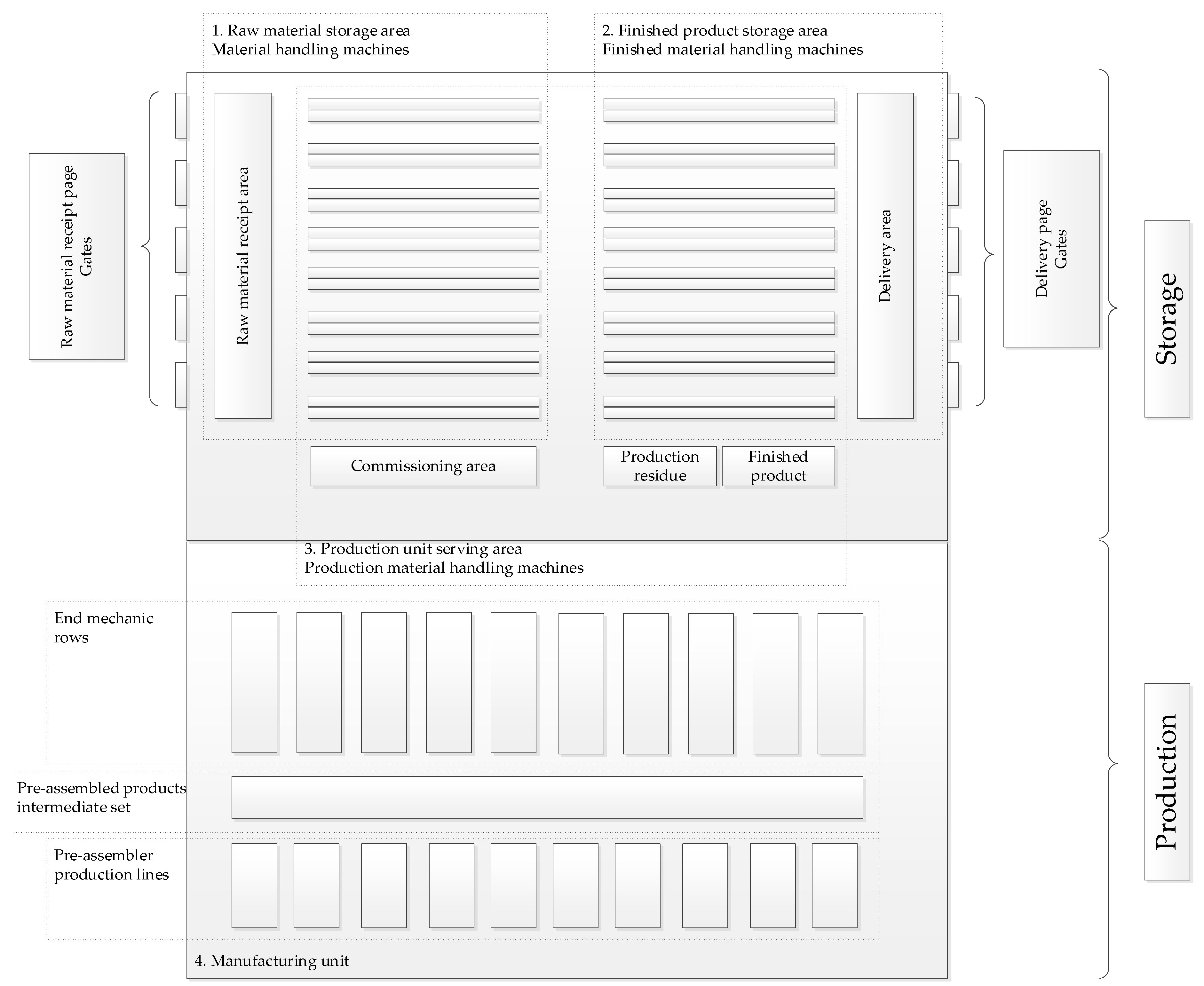
• Reception and storage of raw materials;
• Production area raw material service and material management;
• Storage and delivery of finished product.

Due to the high cost per square meter of production areas, the operation of production equipment is the primary objective in the production areas and while minimizing stocks of raw materials and semi-finished and finished products. In order to ensure the continuous supply of raw materials for production, the service needs of production equipment and processes should be taken into account. These needs have a significant influence on the processes of entry into storage, stocking of raw material, and stocking and removal of finished product.

The model outlined above can be divided into four main parts, which build on each other to form an entire system, ensuring the most important input data and procedures for optimum search, as shown in Figure 1.

Determining the structure and parameters of the warehouse system and creating the necessary data structures provide the basis for the cost model, the backup data of which are evaluated during optimization. Therefore, the method relies, to a large extent, on the widespread application of the Industry 4.0 concept in a given company [21,22], as this is an almost indispensable condition for the development of data structures in sufficient detail and for the effective application of the cost model and optimization process based on it. In addition, the other pillar of the developed method is the comparability of well-known entry and removal strategies to meet the needs of production areas. In each of the material handling steps within the value stream, the cost impact of entry and removal strategies is evaluated. This makes it possible to examine a number of alternatives. The mathematical model proposes the selection of the optimal material handling strategy while minimizing the fixed and variable costs per material movement path.

By minimizing both the required amount of raw material stocks and the lengths of the material movement paths, a significant reduction can be achieved in terms of energy and raw material usage, which can effectively reduce the ecological footprint of a manufacturing company, thus achieving a higher level of environmental sustainability. While this also has the secondary benefit of reducing the associated costs related to the usage of these commodities, it is probably much more important that in recent years, both regulations and investors themselves have increasingly been demanding the realization of sustainable operation from corporations. This can directly impact the economic success of manufacturing companies, as the obtainable amount of investment plays a central role in the business strategy of any firm, and in recent years, a trend is clearly emerging where investors increasingly favor sustainable businesses while reducing their investment portfolio in less sustainable areas of the economy. Therefore, the main interest of manufacturing firms is ultimately to quickly transition to a fully sustainable mode of operation as soon as possible, and the above outlined method can serve as one of the tools to achieve this goal (of course, together with the use of completely carbon-neutral energy sources, the electrification of the entire supply chain, the implementation of recycling as widely as possible, etc.).

Based on the above, two main hypotheses can be identified, which are: (1) By selecting the operational strategy of demand-driven warehousing systems using an inspection system, a more efficient operation can be achieved with regard to internal warehousing processes; (2) in the selection of the warehouse material handling strategy, the integrated management of the processes can directly determine the operation requiring fewer human and mechanical resources, and indirectly the operation requiring less energy and raw material input. These hypotheses are verified through the development and application of a test system. The paper does not detail all the elements of the concept for easier understanding; rather, it contains mainly simplifications thereof.

2. Overview of the Area of Storage System Design

The role of logistics systems is key for all supply chains, as this ensures that materials are delivered from their place of production to consumers [23,24,25,26,27,28,29,30,31,32,33]. Several methods increase the efficiency of a logistic system, e.g., the Lean [34]. Logistics systems are also critical to their role within the production company, as they represent significant value for committed capital [35]. Data for the USA show that the capital and operating costs of warehouses account for about 22% of logistical costs [36], while data for Europe show a similar 25% [37].

A study carried out in the United Kingdom showed that the number of large new warehouses increased steadily between 1995 and 2018 [38,39]. The number of warehousing businesses across Europe shows a similar growth trend in the period 2000–2018 [29]. These warehouses represent significant investments for companies. Expenditure on warehouse automation has been steadily increasing in Europe [40], and this trend is reflected globally by figures showing that sales increased by an average of 5% in the period 2003–2005 [35].

For business success, it is essential that warehouses be designed to operate cost-effectively. This is particularly important as storage costs should be largely determined at the planning stage [41].

Consequently, it is no coincidence that the design of warehouse systems as a comprehensive area has scientific literature dating back several decades. Some of these are mentioned chronologically [35,42]. Heskett (1973) divided the determination of requirements, the design of the material handling system, and the design of the arrangement into three parts [43]. Apple (1977) found that when designing buildings, the designer faces a complex task due to the interactions and relationships between individual design activities. The author defined a 12-step model [44]. According to Ashayeri and Gelders (1985), the most practical basis for warehouse design optimization is the combination of analytical models and simulation. The authors concluded that few articles deal with the topic of warehouse planning [45]. Muther (1987) defined a multi-step systematic layout design method [46,47,48]. Firth, Apple, Denham, Hall, Inglis, and Saipe (1988) defined a four-step model [49,50]. Hatton (1990) also employs a multi-step procedure for the problem of warehouse design [51]. According to Gray et al. (1992), in order to solve the design problem, iteration between the three levels of decision must be carried out in order to obtain a solution that minimizes the total cost [52]. Mulcahy (1994) published a manual on the operation of warehouses, including the main aspects of planning [53]. Oxley (1994) combined the most important steps of previous authors to create a comprehensive list. It begins with the definition of general system requirements for the supply chain, including factors such as service levels and implementation time limits, data collection, and analysis. It also introduces a new step to determine the unit loads to be used. The following steps concern the development of alternative operating methods, equipment, and layouts. It highlights that warehouse design should focus on storage and management requirements and that the building should be designed on this basis [54]. Duve and Mantel (1996) developed a step-by-step decision support method for LogiTRACE [35]. Govindaraj, Blanco, Bodner, Goetschalckx, McGinnis, and Sharp (2000) focused on processes used by designers and experts in the field. They tried to understand the decisions they make and the processes they follow when developing a project. They claimed that the designer should take into account some very complex compromises. The need for and importance of five steps and its repeating were underlined [55]. Rouwenhorst (2000) argued that the design process usually goes through several consecutive stages. They then continued to analyze tasks within these steps, grouping them into a hierarchical framework based on a top-down approach, identifying through them strategic, tactical, and operational decisions. It was proposed that these three sets of decisions be examined one after the other [41]. Goetschalckx (2001) provided a framework system for systematic warehouse planning and the development of a mathematical model [56]. Hassan (2002) and Waters (2003) once again provided a series of steps that are in many ways similar to those of previous authors, although the former deals primarily with one aspect of the design problem, namely layout [57,58]. Bodner (2002) divided the design process into three main phases. In the first stage, designers carry out preparatory work. The result of this section can be a proposal or a project decision document that the client can accept after possible changes. The second stage involves the design work itself. The result of this phase consists of a design specification. The third stage is the implementation of the design [59]. Rushton, Croucher, and Baker (2006) recognized the importance of flexibility in warehouse design. The step of business needs includes the concept of scenario planning, and this leads to a later, concrete step in evaluating design flexibility. An example of the iterative characteristics of the design process is the calculations of equipment and personnel, which are presented after the layout [60]. Kostrzewski (2012) defined a 22-step model by summarizing and developing previous models [49]. Thomas and Meller’s (2015) guidelines can provide warehouse construction close to the optimal solution. They created a framework and delimited decision variables, determining them to be the size and layout of the transport area, the configuration of the dock door, the shape of the pallet, and the height of the pallet warehouse. A statistical methodology was used to develop their planning guidelines [61].

Despite decades-long literature and the importance of warehouse planning, several literature reviews have concluded that few scientific journals have addressed the applicable systematic approach [35,62,63]. In fact, the systematic analysis of warehouse design subprocesses themselves is addressed in several studies [63,64], in subprocesses, for example, examining the issue of flight planning or the layout of storage systems [64,65]. In contrast, there is no overlapping study between subprocesses to find a possible optimum. Of course, it should be added that by exploiting the possibilities of the Industry 4.0 concept, which has become decisive in recent years, a level of full-scale optimization has become available, which would probably not have been realistically feasible before.

3. Description of the Test Options

As already defined in the introduction, the objective of the research was to develop a method for the selection and operation of the storage material handling strategy and to establish a process through which it is possible to choose the optimum strategy, taking into account the material handling steps within the value stream, where one of the main parameters of optimization is cost. The objectives of the research are based on the:

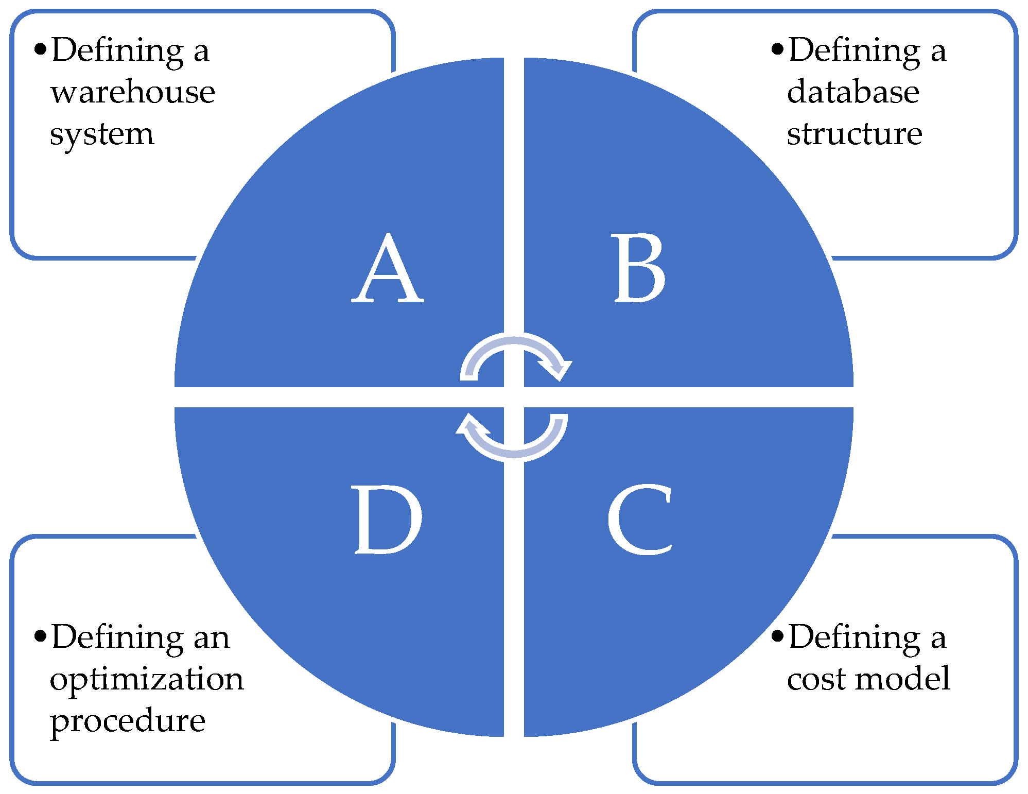
• Development of the concept of a test system to support the optimal selection and operation of the demand-driven storage system;
• Development and calculation of the cost model to support the selection and operation of the demand-driven storage system;
• Definition of the data model, conditions, and purpose function of the test system supporting the selection and operation of the demand-driven storage system.

In order to achieve the former objectives in the sense of the entire warehousing system, a large number of possibilities had to be considered for both the design variants and the operation of the processes. The size of the task is illustrated by the fact that if all variable parameters from the receipt of the raw material through the production processes to the delivery are taken into account, a total of 640,000 test alternatives can be determined using the established approach. Figure 2 illustrates possible system variants in relation to the relationship between entry and removal processes and entry and removal strategies (in the diagram, FIFO means first in, first out; LIFO means last in, first out; FEFO means first expire, first out; LOFO means lowest in, first out; and HIFO means highest in, first out). The loading and unloading strategies and process designation possibilities were elaborated on the basis of the review of the literature [10,11,23,66] as well as our practical experience.

4. Comprehensive Description of the Method Developed

4.1. Presentation of the Concept of Operation of the Test Method

In this section, the structure of the established method is succinctly presented. The high-level operational concept of the test method is described first. The arrayed shape of the system model implementing the method is shown in Figure 3. At the heart of the model is the module for the optimal choice of material handling strategy. The optimization module examines the cost of the entry and removal strategy for each handling step. As mentioned above, 640,000 options are examined during optimization.

The main elements of the model are:

• Information database: It provides input data from the optimization module. These databases contain static background tables of manufactured products and customers that vary with low frequency;
• Picking strategy input data: They provide data for picking processes. On the basis of these data, the claim is determined. The demand generates a to-do list to be executed for the picking operation;
• Entry strategy input data: They provide data for storage processes;
• On the basis of these data, the claim is determined. The demand generates a to-do list to be performed for the picking operation;
• Warehouse database: The database contains static background tables of handling machines, human resources, storage systems, and products that vary with elementary low frequency;
• Business plan database: It is a database of incoming revenues and outcoming expenses or charges required to make a profit, containing information about inventory value and investments.
• Material handling process steps: They are the handling steps during the reception, storage, and removal of the raw material;
• Evaluation database: It contains the results of material handling steps based on entry and removal strategies.

The selection of the optimal warehouse material handling strategy variant is implemented using a simulation test method, which ‘simulates’ the operation of the material flow system according to the different strategy variants using data from a designated past period and a pre-planned period, and then a variant with the most favorable target function value is selected based on the values of the logistic indicators obtained per strategy variant. The steps of the process are illustrated in Figure 4.

The steps in this process can be summarized as follows:

1. Record test data:

The databases required for the study and their contents are outlined below.

To record the elements of the information database:

• Part number and production schedule database data;
• Customer database data;
• Production database;
• Delivery database data.

Data of the elements of the warehouse database:

• Storage system database data;
• Material handling system database data;
• Product database data;
• Human resources database.

Rating details:

• Weight of objective function components;
• Specific cost functions based on historical data;

2. Select interval data: Select the time horizon of the information and warehouse database. Business plan databases provide interval opportunities to select the strategy that meets your expectations. This means that the database data are not static, but their values can be changed within an interval in the amount of available investment, or a limitation is implemented affecting the inventory value, thereby changing the number of operations to be performed, thus affecting the strategy to be selected. Only 1–1 items with an interval value can be selected on both input sides at a time;

3. Initialize interval data: The interval is min. and max. record of the value and the number of step units;

4. Start a simulation program: After recording the data in the data tables, the simulation program is started, which allows you to evaluate the warehouse material handling strategy variant and select the best version for a total of 10 material handling steps based on the given historical and forecasted data. The basic requirement for the simulation program is the automatic creation of the examined system based on past and future data, the running and evaluation of all material handling strategy versions, and the selection of the appropriate version;

5. Create an automatic test model:

Based on the test data, the tested logistics system is created automatically (material handling system, storage system, start-up stocks);

6. Initialize the value of variables: In the simulation test model, two basic variables are initialized, namely v, which contains the material handling strategy variants under study, and Opt, which contains the identifier of the optimal variant. Of course, there are other technical variables used in programming that need to be initialized, but these are not covered now;

7. Define logistics indicators for version v: In this step, the logistics indicators on which the comparison is based are generated (e.g., warehousing costs);

8. Record the data of specific logistics indicators: The values of the logistics indicators defined for each material handling strategy variant are recorded in a predefined data table, on the basis of which the target function components can be normalized later (step 11) and the target function can be generated;

9. Examine whether all possible variations have been examined:

If yes, the process of selecting the optimal version follows; if not, the next version is examined;

10. Increment the material handling strategy variant ID;

11. Normalize objective function components:

The value of the objective function of strategy variant v is determined on the basis of the values of the logistics indicators determined by the simulation model. In order for indicators of different dimensions to be applicable as objective function components, they must be normalized. The optimal material handling strategy is then selected by determining the weighted sum of the normalized objective function components;

12. Record normalized data:

The normalized version of the values of the logistic indicators defined for each material handling strategy variant is recorded in a predefined data table;

13. Determine the optimal version ID: Determine the ID of the optimal version through the objective function.

In order for the presented concept to be truly functional, of course, it is also necessary to have a data structure that serves as the basis for the use of the presented system model. In some ways, this data model is one of the most important parts of the whole process, since without constantly updated dynamic data and extensive hysterical data, effective optimization cannot be imagined. It is also clear that the continuous updating of the data structure requires a wide-ranging implementation of the Industry 4.0 concept in the given company, as this is the only way to ensure that accurate data are used during optimization. The structure of the data model is shown in Figure 5 on the next page.

The starting point of the data structure is the business plan, which shows the general ledger result of the company, taking into account the projected sales value and expenses. Expenses include financing elements of warehouse databases. The plan shows the maximum investment, committed capital, and value-creating operations that achieve the highest operating profit [67,68,69].

The information database determines the needs for warehouse processes. The database is closely related to business planning and the planning of operational production management processes.

The forecast of customer orders determines the range of products to be manufactured and shows a distribution in the change of demand within the calendar year. The processing and scheduling of this forecast generates a ‘demand’ for the ordering of raw material and the receipt of raw material after feedback from suppliers. The receipt schedule provides information as input data about the material to be handled by logistical processes. Smoothing the confirmed arrival times provides an additional opportunity in the optimization process, but the later model does not cover this.

The use of stocked raw material for production is carried out by scheduling customer orders into production, which is based on the date of fulfillment of the order. The date of delivery of the product to the customer, the distance of the delivery address from the production site, the number of products already manufactured in stock, and the production lead time determine when the product enters production. The preparation of the production refinement can be further optimized through a ‘pull’ system and in combination with smooth production, which also has a positive effect on the schedule ability of logistics processes, but this optimization option is not covered by the model.

The manufactured products are packaged differently at the request of customers. The number of finished products that can be placed in customer packaging and the number of raw materials per unit of packaging differ in most cases; therefore, after the production of the finished product in the production plan, the remaining raw material is returned to the storage. The aim is to avoid overproducing and using raw materials from other finished products to be manufactured.

In the foregoing, a comprehensive description of the data model was provided. The main data objects presented contain additional data elements separately, but they are not presented in detail within the framework of this publication, except for part of the information database.

4.2. Presentation of the Cost Model Supporting the Selection and Operation of the Storage System

One of the most important indicators for choosing the optimal warehouse handling strategy is cost, which is one of the most important indicators for comparing the alternative options outlined during the test. When selecting a warehousing strategy, the aim is to operate at the lowest possible cost, which means the expenditure in the entire warehousing process.

Warehouse-related costs can be divided into two parts:

• Variable cost: Every cost element that changes in the event of a change in the warehouse charge in the number of products handled. The following costs can be classified in this category:

  o

  Wage costs: The wages of persons performing the main operational logistical tasks of warehouses, which may vary depending on the warehouse load;

  o

  A certain part of the cost of operation, since with non-continuous operation, overhead costs for example electricity can be reduced by switching off the out-of-service lighting;

  o

  In the case of leasing contracts, the number of leased assets or storage facilities may also be changed. The cost implications and possible reaction time are displayed according to the terms of the contract;

• Fixed costs: all cost elements that cannot be changed in the event of a change in the warehouse load in the number of products moved:

  o

  Some of the operating costs, such as heating of buildings, supply of energy, and maintenance of security services, since a basic level of service must be maintained even if the warehouse is not in operation [70];

  o

  Amortization cost of machinery, equipment, and warehouse building owned by the company.

The steps for determining the costs describing the storage activity are as follows [66]:

Step 1.

Outline the layout model of the warehouse. It is necessary to specify the number of machines involved in the service; the type and capacity of equipment; the number of gates on the arrival and delivery side; and the size and location of the auxiliary areas, for instance, picking area, residual production area to be re-stored, finished production area to be put into storage. Assignments should be focused on the assignment of machines to activities, and delimitations should be made in the orientation of material handling;

Step 2.

Assign item items specified in the first point to the outlined warehouse layout model, such as assigning the number of machines to the raw material receipt page. The cost of each item element and its specific value per day should be determined. These costs are included in the business plan and can therefore be easily specified after groups have been trained;

Step 3.

Define load functions for warehouse processes. These load functions can be used to determine the value-added cost of the warehouse processes performed;

Step 4.

Define inefficiency indicators based on historical data taking into account measures to improve the efficiency of future processes;

Step 5.

Define specific cost functions using clustered unit cost, load functions, and inefficiency indicators. The clustered unit cost can be interpreted for three areas, namely raw material storage processes, production-related raw material handling, and finished product inventory processes. The clustered unit costs are determined using predefined data sets for these subprocesses;

Step 6.

Define logistical indicators for performance measurement;

Step 7.

Determine the inventory value of committed capital. The capital committed in the raw material is one of the largest sources of loss for the company, and therefore, its value should be minimized. The cost of handling materials changes in parallel with the minimization of inventory, as a smaller level of raw material stock requires more frequent and smaller amounts of supply; therefore, it has a significant impact on the selection of the ideal material handling strategy;

Step 8.

Define economic indicators to measure financial performance.

4.2.1. Step 1—Warehouse Layout Model

The structure of a typical warehouse layout model is shown in Figure 6. The arrangement of the shelving systems and the auxiliary areas in the storage area have been determined. The orientation of the material flow is indicated by three blocks: (1) raw material arrival side and storage area, (2) finished product delivery side and storage area, and (3) production unit serving area. The production unit includes end-assembly lines, area of the intermediate set of pre-assembly lines, and pre-assembly production lines. Within the areas, the machine numbers are determined and assigned.

4.2.2. Step 2—Assigning of Items to the Outlined Warehouse Layout Model

The material handling costs are determined on an annual basis for the previous three groups and broken down into daily unit costs. The description of all cost elements would exceed the limits of this article, so as an example, only the cost elements of the raw material area are presented, which are the following (the other cost elements are formulated following a similar logic):

$$ATk=\frac{AEEk+AGGk+ARBk+RUk}{365} (\mathrm{EUR}/\mathrm{year})$$

(1)

where:

• $ATk$—raw material area cost;
• $AEEk$—human resources annual cost—raw material area is relevant;
• $AGGk$—cost of raw material handling machines;
• $ARBk$—cost of warehouse equipment—raw material area is relevant;
• $RUk$—warehouse operating cost—raw material area is relevant.

All cost elements and their relationships are comprehensively illustrated in Figure 7.

4.2.3. Step 3—Definition of Load Functions for Warehouse Processes

The load functions defined for warehouse processes are classified in clusters identical to the number and properties of the groups formed in the previous point. It should be noted that two types of raw material storage processes can be distinguished, namely the normal process (where items are stored directly upon receipt) and non-normal process (e.g., unidentified shipment, shipment awaiting quality control, blocked receipt).

The schematic structure of the load functions is illustrated in Figure 8. Again, it is simply not possible to describe every load function in the model in detail within a single paper, but as an example for the general structure of the functions, the raw material storage normal process time vector is formulated as follows:

$$A{B}_{normal}=\left[A{B}_{normal}^1;A{B}_{normal}^2;\dots ;A{B}_{normal}^{365}\right] (\mathrm{Hour})$$

(2)

where:

• $A{B}_{normal}^n,n\in \left\{1,2\cdot \cdot \cdot 365\right\}$—the storage time requirement for normal raw material on the n-th day of calendar days. The number of calendar days can be set from 1 to 365 as desired.

The normal raw material storage time requirement for n-th calendar day is detailed in the following:

$$\begin{array}{cc}A{B}_{normal}^n=\frac{\frac{{{\displaystyle \sum }}_{ak=1}^{AKa}{{\displaystyle \sum }}_{i=1}^{r_{ak,n}}{l}_{ak}^z}{v}\times 2}{AG{G}_{ak}\times 3600},\hfill & \hfill (\mathrm{Hour})\\ z\in \left\{1,2\cdot \cdot \cdot s\right\},n\in \left\{1,2\cdot \cdot \cdot 365\right\},ak\in \left\{1,2\cdot \cdot \cdot AK\right\}\hfill & \end{array}$$

(3)

where:

• $A{B}_{normal}^n$—normal raw material storage time requirement for n-th calendar day;
• n—index of calendar days;
• ak—index of raw material-side gates;
• $AKa$—number of gates on the raw material side;
• $z$—index of container bin;
• $r_{ak,n}$—ak. number of items to be stored from gate on the n-th day;
• $l_{ak}^z$—the distance of the shortest path from ak. gate to z. bin;
• V—speed of the material handling equipment for entry into storage (m/s);
• $AA{G}_{ak}$—ak. number of material handling machines assigned to the gate.

The related process definitions for the load functions in Figure 8 can be found in the middle column titled ‘Process designation’, in which each definition relates to the abbreviation in the same row of the left column.

4.2.4. Step 4—Definition of Inefficient Indicators Based on Historical Data

There are delays and changes in scheduled material handling for unforeseen reasons that affect loading and removal processes:

• In case of receipt of raw materials, the reason for the change to the planned one may be the arrival of fewer raw materials than the order, delay in delivery due to the weather, technical problems on the supplier’s side, pre-delivery, and so on;
• The causes on the production side may be manufacturing malfunctions, overproduction, batch jumping (batches are not produced according to the pattern specified in the production plan), production of fewer pieces;
• Problems on the delivery side include JIT delivery (the manufactured finished product is loaded directly without entry), technical problems, and transport management problems.

In all three cases, the lack of human resources occurs due to vacation, illness, or fluctuation. To cover the lack of human resources, an additional number of people are included in the business plan, and the additional shortages are addressed by overtime. Therefore, the inefficiency caused by human deficiency in material treatment processes has not been studied by the authors. The derogations listed reduce efficiency, cause uncertainty, and increase costs, so the impact of this should be taken into account. The availability of the listed historical data is a prerequisite for determining inefficiency indicators. Even if these data are not available, inefficient indicators should be defined in accordance with the framework conditions available on the market, as set out in supplier and other contracts. As an example, the inefficiency indicator of page material errors can be described as follows:

$$AHm=1+\left(\frac{AHsz}{\left|{\Theta }_a^n\right|}\times 100\right) (\%)$$

(4)

where:

• $AHm$—inefficient indicator of raw material defects;
• $AHsz$—from historical data, you can specify the standard deviation of batches of raw material arrival errors;
• $\left|{\Theta }_a^n\right|$—on the n-th calendar day, the annual number of items managed by the arrival process $n\in \left\{1;2;\cdot \cdot \cdot ;365\right\},a\in \left\{1;2;\cdot \cdot \cdot ;p\right\}$.

4.2.5. Step 5—Definition of Specific Cost Functions

Specific cost functions are defined using clustered unit cost, load functions, and inefficiency indicators. In this way, the following cost functions have been defined:

• Raw material handling cost;
• Cost of handling production materials;
• Cost of moving finished product;
• Material handling cost.

As an example, the cost of the moving raw material is defined as follows:

$$AMk=\left|AM{k}_1;AM{k}_2;\cdot \cdot \cdot ;AM{k}_n\right| (\mathrm{EUR})$$

(5)

where:

• $AMk$—the cost of the moving raw material;
• $AM{k}_n$, $n\in \left\{1,2,\dots ,365\right\}$—cost of moving raw materials on the n-th calendar day.

$$AM{k}_n=\left(A{B}_{normal}^n\times ATk+a{b}_{jn}^n\times ATk\right)\times AHm (\mathrm{EUR})$$

(6)

where:

• $A{B}_{normal}^n$—the storage time requirement for normal raw materials falling on the n-th calendar day;
• $ATk$—cost of raw material area (per hour);
• $a{b}_{jn}^n$—raw material storage time requirement j. on the n-th calendar day of the non-normal process;
• $AHm$—inefficient indicator of raw material defects.

4.2.6. Step 6—Definition of Logistical Indicators

The definition of logistical indicators helps to determine the percentage of cost in order to measure performance. As the model does not optimize variable costs, the indicators can be used to measure the value of post-intervention performance. After changing the initialization value of variable costs, the model must be run again with the aim of maximizing the value of logistic indicators. The following three logistical indicators have been defined:

• Raw material storage capacity;
• Manufacturing material handling performance;
• Picking performance.

As an example, the raw material storage performance is defined as follows:

$$AT{m}_n=\frac{AM{k}_n}{ATk\times 24}\to max. AT{m}_n\le 100\% [\%]$$

(7)

where:

• $AT{m}_n$—raw material storage capacity on the n-th calendar day;
• $AM{k}_n$—cost of moving raw materials on n-th calendar day;
• $ATk\times 24$—cost of raw material area (per day—the cost per hour must be multiplied by 24 to get the value per day; however, the projection base can be adjusted according to the test needs).

A condition is that its value cannot be greater than 100%. In this case, reducing fixed costs will result in a loss of capacity that requires over-one capacity. In this case, the initialization value of fixed costs should be increased, and the model run again.

4.2.7. Step 7—Determination of the Stock Value of Committed Capital

Figure 9 shows the cost of capital employed, which can be divided into three major parts (raw material inventory value, finished product inventory value, fixed inventory value) as shown in the figure.

As an example, the raw material inventory value is calculated as follows:

$$AKe=\left|AK{e}_1;AK{e}_2;\cdot \cdot \cdot ;AK{e}_n\right| (\mathrm{EUR})$$

(8)

where:

• $AKe$—raw material inventory value;
• $AK{e}_n$—value of raw material in stock on the n-th day.

$$\begin{array}{cc}\hfill AK{e}_n=AI{e}_n+\left({\displaystyle {\displaystyle \sum }_{k=1}^j}{r}_{kn}\times A{e}_{kn}\right)-\left(r_{kon}\times A{e}_{hn}^{ki}\right)+\left(rko{v}_{hn}\times AK{e}_{hn}^{be}\right)+\hfill & \hfill (\mathrm{EUR}/\mathrm{day})\\ \hfill +\left(ra{m}_n\times AM{e}_n^{be}\right)\hfill & \end{array}$$

(9)

where:

• $AI{e}_n$—value of initial raw material stock on the n-th calendar day;
• $r_{kn}$—number of items to be stored from k. gate on the n-th day;
• $A{e}_{kn}$—value of items to be stored from k. gate on the n-th day;
• $rk{o}_{hn}$—number of items to be unloaded for the h picking area on the n-th calendar day;
• $AK{e}_{hn}^{ki}$—value of items to be unloaded for the h picking area on the n-th calendar day;
• $rko{v}_{hn}$—number of items to be stored from the h. picking area on the n-th calendar day;
• $AK{e}_{hn}^{be}$—value of items to be stored from the h. picking area on the n-th calendar day;
• $ra{m}_n$—number of items of residual raw materials of production to be stored on the n-th calendar day;
• $AM{e}_n^{be}$—value of items of residual raw materials of production to be stored on the n-th calendar day.

4.2.8. Step 8—Definition of Economic Indicators

Three economic indicators were introduced in the model: The raw material value indicator, the finished product value indicator, and the non-moving inventory value indicator.

The raw material value indicator is calculated as follows:

$$AE{m}_n=\frac{AK{e}_n}{UAKe÷365} (\%)$$

(10)

where:

• $AE{m}_n$—raw material value indicator on the n-th day;
• $AK{e}_n$—value of raw material in stock on the n-th day;
• $UAKe÷365$—value of the raw material specified in the business plan (for one calendar day).

The value indicator for the finished product is defined as follows:

$$KE{m}_n=\frac{KK{e}_n}{UKAKe÷365} (\%)$$

(11)

where:

• $KE{m}_n$—value indicator for the finished product on the n-th day;
• $KK{e}_n$—value of finished product in stock on the n-th day;
• $UAKe÷365$—the value of the finished product as defined in the business plan (per calendar day).

Finally, the non-moving inventory value indicator is defined as the following:

$$NMKm=\frac{NMKe}{UKAKe} (\%)$$

(12)

where:

• $NMKm$—the non-moving inventory value indicator;
• $NMKe$—average non-moving inventory;
• $UKAKe$—raw material value indicator as defined in the business plan.

4.3. Data Model, Conditions, and Target Function of the Test Method Supporting the Selection and Operation of the Storage System

In order to examine the optimal storage strategy of the storage system, it is necessary to define the framework conditions for the data used as input information, to standardize the type of data, so that all the information is always available for the analysis, on the basis of which the appropriate proposal can be selected. In order to be run and evaluated quickly at specified intervals, this framework is also expected to be defined. Figure 10 illustrates the database structure, which can be divided into three major parts:

• A business plan database based on the number of orders predicted by customers;
• The information database that translates the expectations of the business plan into operational tasks, which generates the needs for logistics processes;
• Warehouse database containing cost elements and edge conditions of the framework required to perform operational tasks.

The established database structure plays a key role in the applicability of the method, as it allows the use of large amounts of continuously generated data in value stream-oriented optimization, thus achieving one of the most important application advantages of the Industry 4.0 concept, i.e., the use of large amounts of data in optimization based on the current real state. For this reason, however, a detailed description of the entire database structure would go beyond the scope of this publication; therefore, only some of the main database elements shown in the former figure are presented, and more specifically the part of the number of pieces and production scheduling database concerning the storage processes.

4.3.1. Information Database: Number and Production Scheduling Database for Storage Processes

The production of fixed orders after customer forecasts must be scheduled, which is preconditioned for the available raw material and the time of receipt to customers. The following matrices and data vectors are required to determine the timing of the receipt of the raw material.

Input incorporation matrix for customer returns:

$$VMAIncorporation=\left|\begin{array}{cccc}vma{b}_{11}& \cdot & \cdot & vma{b}_{1a}\\ \cdot & \cdot & & \\ \cdot & & \cdot & \\ vma{b}_{k1}& & & vma{b}_{ka}\end{array}\right|$$

(13)

where:

• $VMAIncorporation$—input incorporation matrix for customer returns;
• $vma{b}_{ka}$—number of a. snap-in material of k. finished product.

A finished product also contains individual substances or materials common to other finished products. In the event that the finished product (k) is not a snap-in part of the raw material, $vma{b}_{ka}=0$.

Daily basic data matrix of the raw material to be ordered:

$$MA{A}^n=\left|\begin{array}{cccc}ma{a}_{11}^n& \cdot & \cdot & ma{a}_{1a}^n\\ \cdot & \cdot & & \\ \cdot & & \cdot & \\ ma{a}_{k1}^n& & & ma{a}_{ka}^n\end{array}\right|=\left|\begin{array}{cccc}vma{b}_{11}& \cdot & \cdot & vma{b}_{1a}\\ \cdot & \cdot & & \\ \cdot & & \cdot & \\ vma{b}_{k1}& & & vma{b}_{ka}\end{array}\right|\times \left|\begin{array}{c}v{m}_{1n}\\ \cdot \\ \cdot \\ v{m}_{kn}\end{array}\right|$$

(14)

where:

• $MA{A}^n$—daily basic data matrix of the raw material on the n-th calendar day;
• $ma{a}_{ka}^n$—number of a. input raw material required for the ordered number of k. finished products on the n-th calendar day;
• $vma{b}_{ka}$—a. number of inserts of k. finished product;
• $v{m}_{kn}$—number of ordered items with k. ID for the n-th calendar day.

Information vector for raw materials to be ordered on a daily basis:

$$MAA{i}^n=\left|MAA{i}_1^n;MAA{i}_2^n;\cdot \cdot \cdot ;MAA{i}_a^n\right|$$

(15)

where:

• $MAA{i}^n$—information vector for raw materials on the n-th calendar day;
• $MAA{i}_a^n$—amount of a. raw material to be ordered on the n-th calendar day.

$$MAA{i}_a^n={\displaystyle \sum }_{k=1}^{p}ma{a}_{ka}^n$$

(16)

where:

• $ma{a}_{ka}^n$—number of a. built-in raw materials required for the ordered number of finished products on the n-th calendar day

Information matrix of raw materials to be ordered:

$$MAi=\left|\begin{array}{c}MA{A}^1\\ MA{A}^2\\ \cdot \\ MA{A}^n\end{array}\right|=\left|\begin{array}{cccc}maa{i}_{11}& \cdot & \cdot & maa{i}_{1a}\\ \cdot & \cdot & & \\ \cdot & & \cdot & \\ maa{i}_{n1}& & & maa{i}_{na}\end{array}\right|$$

(17)

where:

• $MAi$—information matrix of raw materials;
• $maa{i}_{na}$—number of a. raw material required for the n-th calendar day.

The palletization of the raw material required for the manufacture of the finished product depends on the packaging specification of the material, and this also determines the number of raw materials received on one pallet.

Vector of packaging specification (number of raw materials within unit cargo per raw material):

$$CSe=\left|CS{e}_1;CS{e}_2;\cdot \cdot \cdot ;CS{e}_a\right|$$

(18)

where:

• $CSe$—vector of packaging specification;
• $CS{e}_a$—a. number of raw material within a unit load (pallet).

Pallet number matrix of raw materials to order:

$$MAr=\left|\begin{array}{cccc}ma{r}_{11}& \cdot & \cdot & ma{r}_{1a}\\ \cdot & \cdot & & \\ \cdot & & \cdot & \\ ma{r}_{n1}& & & ma{r}_{na}\end{array}\right|=\left|\begin{array}{cccc}maa{i}_{11}& \cdot & \cdot & maa{i}_{1a}\\ \cdot & \cdot & & \\ \cdot & & \cdot & \\ maa{i}_{n1}& & & maa{i}_{na}\end{array}\right|÷\left|CS{e}_1;CS{e}_2;\cdot \cdot \cdot ;CS{e}_a\right|$$

(19)

where:

• $MAr$—pallet number matrix of raw materials;
• $ma{r}_{na}$—number of pallets containing a. raw material required on the n-th day;
• $ma{a}_{ka}^n$—number of a. built-in raw material required for the ordered number of k. finished products on the n-th calendar day.

The information matrix of the raw materials to be ordered contains the number of raw materials required for the production of the ordered finished product on a daily basis. In this case, if the production lead time of the finished product, the production and delivery times of the suppliers, and the stocking lead time of the raw material were zero, the planned arrival matrix of the raw material and the information matrix of the raw materials to be ordered would be the same. Otherwise, the said particulars must be provided in order to plan the receipt of the raw material.

Matrix of lead time for the supply of raw materials by supplier:

$$ABA{i}^k=\left|\begin{array}{cccc}ab{a}_{11}^k& \cdot & \cdot & ab{a}_{1a}^k\\ \cdot & \cdot & & \\ \cdot & & \cdot & \\ ab{a}_{s1}^k& & & ab{a}_{sa}^k\end{array}\right|$$

(20)

where:

• $ABA{i}^k$—matrix of lead time for the supply of raw materials;
• $ab{a}_{sa}^k$—delivery time of the a. built-in material supplied by the s. supplier of the k. finished product.

Due to the different local location, production lead time, and production depth of the suppliers, the delivery time of each raw materials varies considerably.

Matrix of supplier performance of raw materials:

$$ABT=\left|\begin{array}{cccc}ab{t}_{11}& \cdot & \cdot & ab{t}_{a1}\\ \cdot & \cdot & & \\ \cdot & & \cdot & \\ ab{t}_{1s}& & & ab{t}_{as}\end{array}\right|$$

(21)

where:

• $ABT$: matrix of supplier performance of raw materials;
• $ab{t}_{as}$—a. material daily capacity supplied by the s. supplier.

Supplier performance determines the size of the item that can be fulfilled in one day. This means that if $ab{t}_{asz}=100$ and the size of the regulation item is 300pc by day n, the first delivery item must be received $n_b=n-\frac{300}{100}=n-3$.

Matrix of production lead time:

$$GYAi=\left|\begin{array}{cccc}gya{i}_{11}& \cdot & \cdot & gya{i}_{1gy}\\ \cdot & \cdot & & \\ \cdot & & \cdot & \\ gya{i}_{k1}& & & gya{i}_{kgy}\end{array}\right|$$

(22)

where:

• $GYAi$—matrix of production lead time;
• $gya{i}_{kgy}$—lead time of the k. finished product to be produced on the gy. production line.

The production of finished products can be carried out simultaneously on several production lines. The permeability of production lines varies significantly due to their purchasing time, technological capability, and production depth; therefore, the production lead time of the k-th finished product may vary over different production salts. If k-th finished product gy. cannot be produced on the production line, its value is $gya{i}_{kgy}=0$.

Vector of average inventory (storage) time:

$$aKi=\left|aK{i}^1;aK{i}^2;\cdot \cdot \cdot ;aK{i}^a\right|$$

(23)

where:

• $aKi$—vector of average inventory (storage) time;
• $aK{i}^a$—average storage time of a. raw material.

The raw materials must be received before manufacture. In order to continuously supply production, the receipt of the raw material is timed and carried out earlier than the beginning of production.

Lead matrix of the average material treatment time:

$$aAAi=\left|aAA{i}^1;aAA{i}^2;\cdot \cdot \cdot ;aAA{i}^a\right|$$

(24)

where:

• $aAAi$—lead matrix of the average material treatment time;
• $aAA{i}^a$—average treatment time of a. raw material, which means the time of material handling inside the storage and outside and inside the production line.

In order to be available on the n-th day in the matrix of pallet numbers of raw materials to be ordered, the raw material must be received on $n-x$. day.

The relationships between the handling cost performance and the mode of control is summarized in Figure 11. Again, it is not possible to detail all listed functions in the scope of this paper, but the previously described relations showcase the general logic behind the structure of the listed elements. As in the case of Figure 8, the related process definitions for the abbreviations in the leftmost column can be found in the column titled ‘Process designation’, which in this case is the rightmost column.

The pallet number matrix of the receipt of raw materials:

$$AIncome=\left|\begin{array}{cccc}a{p}_{11}& \cdot & \cdot & a{p}_{1n}\\ \cdot & \cdot & & \\ \cdot & & \cdot & \\ a{p}_{a1}& & & a{p}_{an}\end{array}\right|$$

(25)

where:

• $AIncome$—the pallet number matrix of the receipt of raw materials;
• $a{p}_{nv}$—number of a. ID item palette received on the n-th calendar day.

$$vAIncome=\left|vAIncom{e}^1;vAIncom{e}^2;\cdot \cdot \cdot ;vAIncom{e}^n\right|$$

where:

• $vAIncom{e}^n$—sum of the number of raw materials received on the n-th calendar day.

$$vAIncom{e}^n={\displaystyle \sum }_{a=1}^{p}a{p}_{an}$$

(26)

Data controlling the normal process of raw material storage: number of raw materials to be stored from ak. gate on a daily basis:

$$r_{ak,n}=\frac{vAIncom{e}^n}{AK}$$

(27)

where:

• $r_{ak,n}$—number of raw materials to be stored from ak. gate on the n-th calendar day;
• $AK$—number of gates on the raw material side.

Vector of the physical dimension of the unit cargo of the raw material:

$$AFD=\left|AF{D}^1;AF{D}^2;\cdot \cdot \cdot ;AF{D}^a\right|$$

(28)

where:

• $AFD$—vector of the physical dimension of the unit cargo of the raw material;
• $AF{D}^a$—a. material dimensionalization parameters.

4.3.2. Relationship between Material Handling Cost Performance and Control Mode

As shown in the previous subsection, the data in the database determine the logistical operations to be performed and the costs of the processes. It was also observed that the elements of the database can be divided into two parts: data controlling entry into storage and data controlling picking. Of course, the former applies to all elements of the database, not only to the previously described elements of the information database. Figure 11 presents the relationship between the performance of the material handling cost and the method of control throughout the entire database.

4.3.3. Target Function of the Method for Selecting an Optimal Warehouse Handling Strategy Controlled by Demand

As has been highlighted several times, costs are the basis for choosing the optimal material handling strategy. During optimization, the storage (4 variants) and picking (5 variants) strategies are compared based on the movement of finished products and materials of different states necessary for the supply of customers in the business plan. The cost is based on fixed and variable costs in the business plan. The conditions to be defined for optimization are as follows:

• Determine the level of initialization of warehouse equipment, machinery, and human resources. Record the number of warehouse locations and service machines and the need for the necessary human resources;
• Carry out the movement operations planned for the n-th calendar day within the n-th day. In the event that the available capacity is not sufficient to perform the operations, the initialization level shall be increased, and the optimum search shall be carried out again;
• Customer orders included in your stores plan will be leveled within calendar years, avoiding peak periods.

In addition to defining the conditions, based on the previous steps of the method, the following logistical indicators are required to specify the target function:

• Logistic material handling cost indicator;
• Logistic performance indicator;
• Committed capital cost indicator;
• Inventory value indicator;
• Adaptability index.

As an example, the logistic material handling cost indicator can be defined as follows:

$$L{G}^V=\frac{{\sum }_{n=1}^{365}AM{k}_n+{\sum }_{n=1}^{365}GYM{k}_n+{\sum }_{n=1}^{365}KM{k}_n}{\left(ATk\times \left(GYTk+KTk\right)\right)\times 365}$$

(29)

where:

• $L{G}^V$—logistic material handling cost indicator;
• $AM{k}_n$—cost of moving raw materials on the n-th calendar day;
• $ATk$—area cost of raw material (per day);
• $GYM{k}_n$—cost of handling materials on the n-th calendar day;
• $GYTk$—cost of production area (per day);
• $KM{k}_n$—the cost of moving the finished product on the n-th calendar day;
• $KTk$—area cost of finished product (per day).

The logistics material handling cost indicator shows the cost ratio generated by the loading and unloading V. strategy in relation to the total cost. V. strategy is an identifier for a loading and unloading strategy that represents a combination of the loading and unloading strategy for the process steps.

The only parameter in the target function is the identification of the material handling strategy variant. In fact, the target function selects the most favorable variant (Opt) based on the weighted sums of the normalized target function components defined for the material handling strategy variants—normalized logistical indicators—and determines its target function value (C). Based on this, the target function can be written in the following form:

$$C=\underset{v}{min}\left\{{\sum }_{l=1}^5{w}_l\times Y_i^V\right\},\mathrm{where}0\le w_l\le 1\mathrm{and}{\sum }_{l=1}^5{w}_l=1$$

(30)

where:

• $C$—target function value for the optimal material handling strategy variant;
• $v$—ID of the tested material handling strategy variant;
• $l$—target function component ID;
• $W_l$—target function component $l$. Weight;
• $Y_i^V$—V. Version $l.$ target function component value.

5. Application of the Established Method

The practical applicability of the established method and the correctness of the established relationships were demonstrated through the use of simulation modeling. During the simulation, the structure of the test system was created, and the initial values of the necessary data tables were initialized. Through the explored multi-step cost model, fixed and variable cost values for material handling strategies were calculated. Using the values obtained, the optimal material handling strategy was selected after executive optimization.

Due to the scope of the method, the framework of the publication does not allow the presentation of the entire calculation process; therefore, only the simulation algorithm, as well as the delimitation of the simulation environment and the final result are presented. At the same time, a detailed description of the initial data tables and a description of the entire optimization process can be found together [66].

5.1. Operating Algorithm of the Simulation Program That Selects the Material Handling Strategy

The simulation process for selecting the material handling strategy can be structurally divided into four parts:

• Define the structure of the warehouse system and determination of the data of the structural elements;
• Upload the data structure of the material handling system (from the recording of the test data);
• Write up and calculate items in a cost model;
• Perform optimization.

5.1.1. A. Definition of the Structure of the Warehouse System and Determination of the Data of the Structural Elements

• From the structure of the storage system shown in Figure 12, it is necessary to select the elements for which the test is to be carried out.
• For the selected test elements, the warehouse parameters must be determined:

  o

  Selected warehouse size;

  o

  Warehousing structure;

  o

  Physical parameters of warehouse characteristics (for example, distance of storage space).

5.1.2. B. From the Topping of the Data Structure of the Material Handling System (From the Recording of the Test Data)

The databases specified in Section 4.3 shall be uploaded with data.

The business plan database:

• Business forecasts database;
• Investment database;
• Limit database.

Elements of the information database data table:

• Number of pieces and production scheduling database for storage processes:

  o

  Raw material incorporation matrix for customer orders;

  o

  Daily basic data matrix of the raw material to be ordered;

  o

  Information vector for raw materials to be ordered on a daily basis;

  o

  Information matrix of raw materials to be ordered;

  o

  Vector of packaging specification (number of raw materials per raw material within unit cargoes);

  o

  Pallet number matrix of raw materials to order;

  o

  Matrix of lead times for the supply of raw materials as our supplier;

  o

  Matrix of supplier performance of raw materials;

  o

  Matrix of production lead time;

  o

  Vector of average inventory (storage) time;

  o

  Lead matrix of the average material treatment time;

  o

  Palette number matrix for receipt of raw materials;

  o

  Vector of the physical dimension of the unit cargo of the raw material;

• Number of pieces and production scheduling database for picking processes:

  o

  Production fine plan matrix;

  o

  Daily base data matrix of the raw material to be opened;

  o

  Information vector for raw materials to be opened on a daily basis;

  o

  Information matrix of raw materials to be opened;

  o

  Pallet number matrix of raw materials to be opened;

  o

  Matrix of rounded pallet numbers of raw materials to be opened;

  o

  Matrix of residual finished product;

  o

  Vector of residual finished product to be opened daily;

  o

  Finished product packing vector;

  o

  Base data matrix of the packing to be opened.

Warehouse database:

• Material handling tools database:

  o

  Database of handling machines;

  o

  A database of properties for handling machines;

  o

  Maintenance database of handling equipment;

  o

  Database of transport capacity of handling equipment;

  o

  A database of handling routes.

• Human resources database:

  o

  Human data database;

  o

  Work schedule database.

• Storage system database:

  o

  Storage system size data database;

  o

  Storage occupancy, matrix of empty storage spaces;

  o

  Type of material in the space.

• Product database:

  o

  Storage positions of start-up stocks by product type;

  o

  Product type placement options.

5.1.3. C. Write up and Calculate Items in a Cost Model

The costs describing the storage activity specified in Section 4.3 should be determined and calculated:

Step 1.

Outline the layout model of the warehouse;

Step 2.

Assign items from the item specified in the first point to the outlined warehouse layout model;

Step 3.

Define load functions for warehouse processes. Use these load functions to determine the value add-on cost for the warehouse processes performed;

Step 4.

Identify inefficient indicators based on historical data taking into account measures to improve the efficiency of future processes;

Step 5.

Define specific cost functions using clustered unit cost, load functions, and inefficiency indicators.

Clustering is an area of unit costs in this regard

Raw material storage processes

Production-related raw material handling

Finished product removal processes

Step 6.

Define logistical indicators for performance measurement;

Step 7.

Determine the inventory value of committed capital;

Step 8.

Define economic indicators to measure financial performance.

5.1.4. D. Perform Optimization

Performing the steps of the system for selecting the material handling strategy specified in Figure 4:

• Record test data;
• Select interval data;
• Initialize interval data;
• Start a simulation program;
• Automatically create a test model;
• Initialize the value of variables.
• Define logistical indicators for the v-ed version;
• Record data for specific logistical indicators;
• Determine whether all possible variations have been examined;
• Increment the material handling strategy variant ID;
• Normalize target function components;
• Capture normalized data;
• Determine optimal version ID.

5.2. Definition of the Simulation Environment

The applicability of the test method presented was verified by means of a mathematical simulation, for which the test environment was delimited as follows:

• Duration of study period: 1 day;
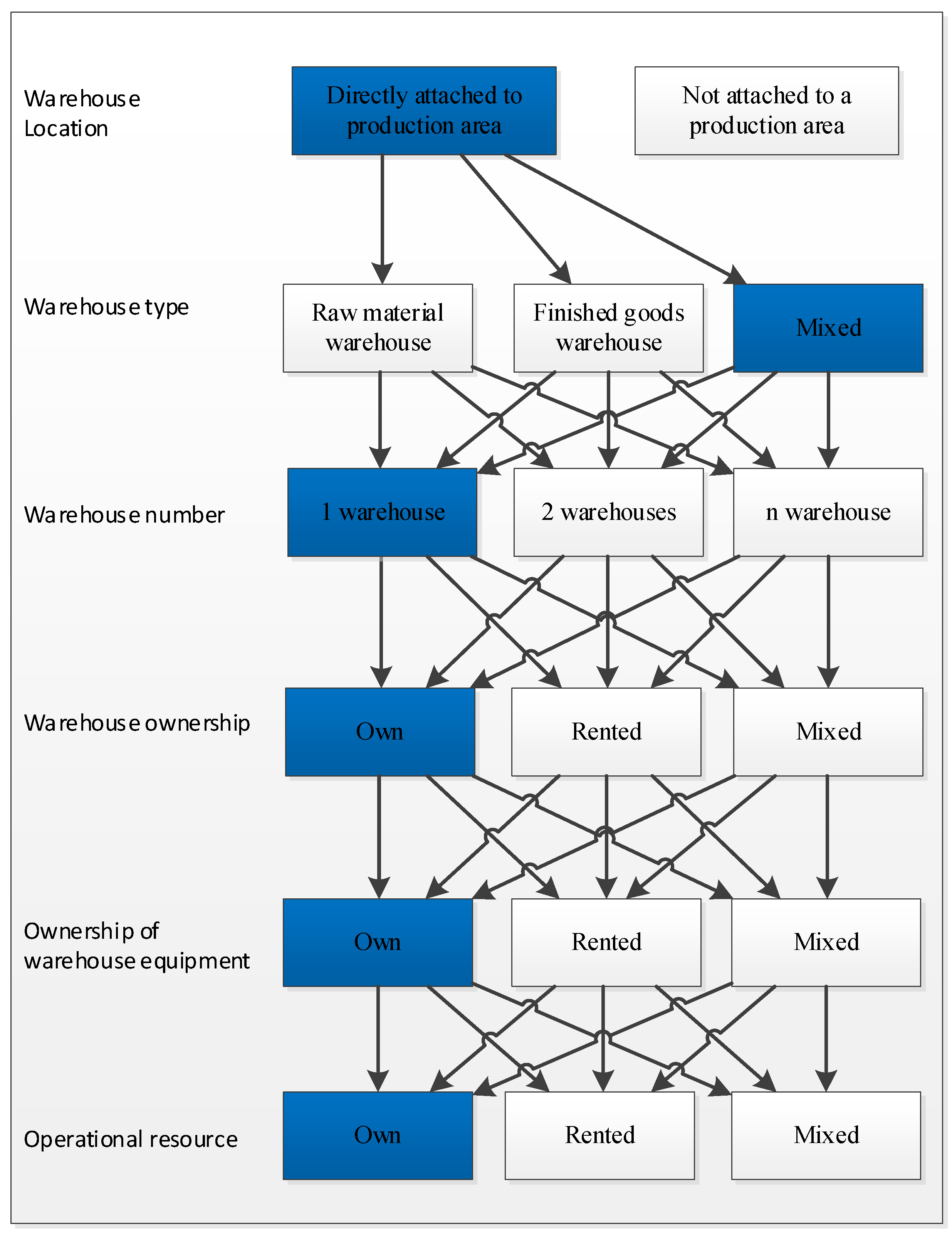
• Warehouse location: Directly attached to production area;
• Warehouse type: mixed;
• Warehouse number: 1 warehouse;
• Warehouse ownership: own;
• Ownership of warehouse equipment: Own;
• Operational Resource: Own;
• Number of handling steps: 2:

  o

  Raw material entry in case of normal process;

  o

  Raw material removal for picking.

The number of combinations tested during the test during the two handling steps is 20. The maximum number of combinations available for all material handling steps is 640,000.

5.3. Define a Target Function

As a result of the simulation carried out, the following values were given, where parameters Y_1..5^V represent the values of the five normalized logistic indicators and C represents the target function (

Table 1. Summary of the results of the mathematical simulation performed.

V. Version Number	Loading Process	Unloading Process	Y1V	Y2V	Y3V	Y4V	Y5V	C
1	Load for nearest open storage	HIFO Unloading	0.9672	0.9360	0.9360	0.8982	1	4.7374
3	Fixed storage loading	HIFO Unloading	0.9721	0.9455	0.9455	0.8982	1	4.7613
2	Loading by class	HIFO Unloading	0.9723	0.9459	0.9459	0.8982	1	4.7623
4	Randomloading	HIFO Unloading	0.9756	0.9522	0.9522	0.8982	1	4.7781
7	Randomloading	FIFO Unloading	0.9764	0.9538	0.9538	0.9174	1	4.8013
6	Fixed storage loading	FIFO Unloading	0.9804	0.9618	0.9618	0.9174	1	4.8215
8	Loading by class	FIFO Unloading	0.9797	0.9603	0.9603	0.9174	1	4.8177
5	Load for nearest open storage	FIFO Unloading	0.9828	0.9664	0.9664	0.9174	1	4.8329
13	Fixed storage loading	LIFO Unloading	0.9868	0.9743	0.9743	0.9469	1	4.8823
10	Load for nearest open storage	LIFO Unloading	0.9878	0.9762	0.9762	0.9469	1	4.8872
14	Fixed storage loading	FEFO Unloading	0.9883	0.9772	0.9772	0.9534	1	4.8960
9	Randomloading	LIFO Unloading	0.9909	0.9824	0.9824	0.9469	1	4.9025
12	Loading by class	LIFO Unloading	0.9918	0.9842	0.9842	0.9469	1	4.9070
15	Load for nearest open storage	FEFO Unloading	0.9875	0.9756	0.9756	0.9534	1	4.8921
11	Randomloading	FEFO Unloading	0.9923	0.9851	0.9851	0.9534	1	4.9159
16	Loading by class	FEFO Unloading	0.9942	0.9889	0.9889	0.9534	1	4.9253
19	Fixed storage loading	LOFO Unloading	0.9957	0.9917	0.9917	1.0000	1	4.9791
17	Loading by class	LOFO Unloading	0.9984	0.9971	0.9971	1.0000	1	4.9927
20	Randomloading	LOFO Unloading	0.9985	0.9973	0.9973	1.0000	1	4.9930
18	Load for nearest open storage	LOFO Unloading	1.0000	1.0000	1.0000	1.0000	1	5.0000

).

To prove this, the most spectacular part of the simulation is the difference between the extreme value of the material handling costs obtained during the combination of the examined loading and unloading strategies:

• Raw material movement cost: 1.95%;
• Production material handling cost: 5.99%;
• Material handling cost: 3.38%.

For the whole simulation, the sequence of entry and removal strategies between the calculation steps during the test is constantly changing, which confirms the impact and necessity of the defined logistical and economic indicators on optimization.

Based on the simulation performed, the lowest cost can be achieved with the version ‘1’ (nearest open storage—HIPO unloading). The highest cost was the ‘18’ (LOFO unloading) version.

As a result of the simulation, it can be concluded that the established system can be used to select the optimal material handling strategy for the demand-driven storage system. As mentioned earlier, a detailed description of the initial data tables and a presentation of the entire simulation process can be found together in [66].

5.4. Outline the Limitations of the Simulation Framework and the Significance of the Results Obtained

The presented test method was developed to determine the optimal material handling strategies of the warehouses in one site integrated with production. These tests can be applied to companies that have a raw material and a finished product warehouse at the site. It will be necessary to extend the model in case there are several raw material warehouses and/or finished product warehouses at the company’s site, and it is necessary to introduce a new type of operation in addition to the specified 10 types of material handling operations.

Based on this, it can be stated that an extremely widely applicable test method has been developed, which can be easily improved if necessary.

As a result of the simulation, it can be demonstrated that the material handling strategy has an impact on material handling costs and ensures the selection of the appropriate cost-effective strategy, providing significant cost savings and predictability for companies using the model.

A significant advantage of applying the test method is that the long-term fixed material handling strategies used so far can be reviewed in a short time, so we can take a significant step toward more efficient company operations.

6. Summary and Conclusions

The efficiency of the market and the difficult and only short-term planning of end-user demand pose an increasing risk to industrial actors and companies. Most industry players are adapting to the new market environment for sustainability, and this adaptation involves reallocations of available financial envelopes, significant cost reductions, austerity, and ultimately restructuring. These listed methods cost a significant amount of internal energy within the company—and while the company focuses on solving its internal problems, it lags behind its competitors. Any reorganization will reduce performance in the short term as previously established information channels change and/or disappear.

For the above reasons, any method or procedure that helps to determine and plan the expected costs based on the available data, relying on the possibilities provided by the Industry 4.0 concept, is therefore a significant help to companies. Adaptation to changed needs can be achieved based on exact data and methods. Perhaps even more importantly, any new method needs to focus on the environmental sustainability of the processes at least as much as on cost optimization, for the reasons outlined in the introduction of this paper.

The developed procedure can be applied to production companies to select a cost-optimized warehousing strategy through the minimization of raw materials and energy usage, taking into account the value of committed capital and investment opportunities in the business plan, ensuring plannability and predictability in terms of costs incurred while lowering the overall ecological footprint the logistics operations.

Possible use of results:

• The warehousing model can be customized for production companies;
• The developed procedure is demand driven, and these needs can be tailored to the individual;
• The needs extend to the handling of raw materials, production, and finished products;
• The number of customer forecasts used in business planning can be used as the main input data;
• The elaborated multi-step cost-prescribing procedure is easy to implement;
• The basis of optimization is the material handling path;
• The model can often be run in search of an optimum;
• By changing the initialization status, you provide an opportunity to reduce costs while choosing the optimal strategy.

The developed test method results in an increase in process efficiency in the field of warehouse material handling. This contributes to reducing the number of resources required, and thus to increasing sustainability. Due to its complexity, the established system includes many possibilities for further development. The primary option is to program the model and create the interfaces needed to adapt it to ERP systems. This allows for an in-stream and online optimal search. Of course, the need for this must be considered, as it is not possible to change the loading and unloading strategy from day to day.

A significant improvement opportunity is the possibility of re-storage during loading and unloading. This means that in the case of fixed storage, the storage of the remaining material after removal is not stored in the same place as storage before removal. In this case, a new fixed storage space is defined, which, for example, makes it possible to reduce the travel path and thereby dynamically smoothen the overloaded periods, as opposed to the static smoothing of the developed model, in order to achieve further cost optimization.

More development opportunities:

• Extend the model to a production company with no attached warehouse;
• Extend optimization to human capacity planning;
• Increase the number of handling operations (more than 10);
• Avoid static pre-leveling;
• Develop applicability to automatic warehouses.

The presented test method was developed to determine the optimal material handling strategies for the warehouses. The method manages production and warehousing processes in an integrated way. These tests can be applied to companies where there is one raw material warehouse and one finished product warehouse at the examined site. It will be necessary to extend the model for cases where there are several raw material warehouses and/or finished product warehouses at the company’s site, and in addition to the specified 10 types of material handling operations, it is necessary to introduce a new type of operation. The implementation of this extended testing program can help in the finalization of certain aspects of the method; for example, it can help in determining the optimal number of examined versions during the optimization process. Another feature that would be necessary for the full applicability of the method would be the quantification of the energy usage in the model, as currently, we can only qualitatively determine that the optimal solution is also the most energy efficient and environmentally sustainable one (based on the fact that it requires the least amount of material handling work and raw material stock). The authors hope that with the further development of the model, these remaining questions can be easily answered.

Together with the few mentioned areas which could be elaborated further in the future, overall, it can be stated that an extremely widely applicable test method has been developed, which can be easily improved if necessary. It should be noted that in addition to the development of the test method, we also laid down the theoretical foundations for a possible combination of warehouse management strategies, which could be the subject of new research.

References

1. Doron, N. EBITDA, EBITA, or EBIT?, Columbia Business School Research Paper 2019, No. 17-71. Available online: https://papers.ssrn.com/sol3/papers.cfm?abstract_id=2999675 (accessed on 27 October 2021).
2. Ferrara, F.; Santilli, P.; Vitiello, A.; Forte, G.; D’Aiuto, V. Logistics management provides greater efficiency, governance and compliance. Int. J. Clin. Pharm. 2021, 43, 1431–1435. [Google Scholar] [CrossRef] [PubMed]
3. Mohammadnazari, Z.; Ghannadpour, S.F. Sustainable construction supply chain management with the spotlight of inventory optimization under uncertainty. Environ. Dev. Sustain. 2021, 23, 10937–10972. [Google Scholar] [CrossRef]
4. Popović, V.; Kilibarda, M.; Andrejić, M.; Jereb, B.; Dragan, D. A New Sustainable Warehouse Management Approach for Workforce and Activities Scheduling. Sustainability 2021, 13, 2021. [Google Scholar] [CrossRef]
5. Ceraolo, M.; Consolo, V.; Di Monaco, M.; Lutzemberger, G.; Musolino, A.; Rizzo, R.; Tomasso, G. Design and Realization of an Inductive Power Transfer for Shuttles in Automated Warehouses. Energies 2021, 14, 5660. [Google Scholar] [CrossRef]
6. Zhang, M.; Luo, Y.; Huang, D.; Miao, H.; Wu, L.; Zhu, J. Maize storage losses and its main determinants in China. China Agric. Econ. Rev. 2021. [Google Scholar] [CrossRef]
7. Giat, Y.; Bouhnik, D. A Decision Support System and Warehouse Operations Design for Pricing Products and Minimizing Product Returns in a Food Plant. Interdiscip. J. Inf. Knowl. Manag. 2021, 16, 39–54. [Google Scholar] [CrossRef]
8. Luo, Y.; Huang, D.; Li, D.; Wu, L. On farm storage, storage losses and the effects of loss reduction in China. Resour. Conserv. Recycl. 2020, 162, 105062. [Google Scholar] [CrossRef]
9. La Scalia, G.; Micale, R.; Miglietta, P.P.; Toma, P. Reducing waste and ecological impacts through a sustainable and efficient management of perishable food based on the Monte Carlo simulation. Ecol. Indic. 2019, 97, 363–371. [Google Scholar] [CrossRef]
10. Ang, M.; Lim, Y.F. How to optimize storage classes in a unit-load warehouse. Eur. J. Oper. Res. 2019, 278, 186–201. [Google Scholar] [CrossRef]
11. Bahrami, B.; Piri, H.; Aghezzaf, E.-H. Class-based Storage Location Assignment: An Overview of the Literature. In Proceedings of the 16th International Conference on Informatics in Control, Automation and Robotics; SciTePress—Science and Technology Publications: Setúbal, Portugal, 2019. [Google Scholar]
12. Pan, C.; Yu, S.; Du, X. Optimization of warehouse layout based on genetic algorithm and simulation technique. In Proceedings of the 2018 Chinese Control and Decision Conference (CCDC), Shenyang, China, 9–11 June 2018; pp. 3632–3635. [Google Scholar]
13. Eder, M. Analytical model to estimate the performance of shuttle-based storage and retrieval systems with class-based storage policy. Int. J. Adv. Manuf. Technol. 2020, 107, 2091–2106. [Google Scholar] [CrossRef] [Green Version]
14. Preghenella, N.; Battistella, C. Exploring business models for sustainability: A bibliographic investigation of the literature and future research directions. Bus. Strat. Environ. 2021, 30, 2505–2522. [Google Scholar] [CrossRef]
15. Chen, S.; Lin, N. Culture, productivity and competitiveness: Disentangling the concepts. Cross Cult. Strat. Manag. 2020, 28, 52–75. [Google Scholar] [CrossRef]
16. Alhawari, O.; Awan, U.; Bhutta, M.; Ülkü, M. Insights from Circular Economy Literature: A Review of Extant Definitions and Unravelling Paths to Future Research. Sustainability 2021, 13, 859. [Google Scholar] [CrossRef]
17. Atif, S.; Ahmed, S.; Wasim, M.; Zeb, B.; Pervez, Z.; Quinn, L. Towards a Conceptual Development of Industry 4.0, Servitisation, and Circular Economy: A Systematic Literature Review. Sustainability 2021, 13, 6501. [Google Scholar] [CrossRef]
18. Noto, G.; Cosenz, F. Introducing a strategic perspective in lean thinking applications through system dynamics modelling: The dynamic Value Stream Map. Bus. Process. Manag. J. 2021, 27, 306–327. [Google Scholar] [CrossRef]
19. Klimecka-Tatar, D. ANALYSIS AND IMPROVEMENT OF BUSINESS PROCESSES MANAGEMENT – BASED ON VALUE STREAM MAPPING (VSM) IN MANUFACTURING COMPANIES. Pol. J. Manag. Stud. 2021, 23, 213–231. [Google Scholar] [CrossRef]
20. Sultan, F.A.; Routroy, S.; Thakur, M. A simulation-based performance investigation of downstream operations in the Indian Surimi Supply Chain using environmental value stream mapping. J. Clean. Prod. 2021, 286, 125389. [Google Scholar] [CrossRef]
21. Silva, N.; Barros, J.; Santos, M.Y.; Costa, C.; Cortez, P.; Carvalho, M.S.; Gonçalves, J.N.C. Advancing Logistics 4.0 with the Implementation of a Big Data Warehouse: A Demonstration Case for the Automotive Industry. Electron. 2021, 10, 2221. [Google Scholar] [CrossRef]
22. Zoubek, M.; Simon, M. Evaluation of the Level and Readiness of Internal Logistics for Industry 4.0 in Industrial Companies. Appl. Sci. 2021, 11, 6130. [Google Scholar] [CrossRef]
23. Kłodawski, M.; Jacyna, M.; Lewczuk, K.; Wasiak, M. The Issues of Selection Warehouse Process Strategies. Procedia Eng. 2017, 187, 451–457. [Google Scholar] [CrossRef]
24. Bányai, T.; Cselényi, J. Logistics Networks–Models and Applications; University of Miskolc: Miskolc, Hungary, 2005. [Google Scholar]
25. Benkő, J. Logisztika II. In Felsőfokú Logisztikai Tanfolyam; Szent István University: Gödöllő, Hungary, 2007. [Google Scholar]
26. Benkő, J. Periodikus készletfigyelésű Modell Megoldása Dinamikus Programozással Általános Feltételek Mellett; Kutatási és Fejlesztési Tanácskozás: Gödöllő, Hungary, 2002. [Google Scholar]
27. Cselényi, J.; Illés, B. Logisztikai rendszerek I.; Miskolci Egyetemi Kiadó: Miskolc, Hungary, 2004. [Google Scholar]
28. Cselényi, J.; Illés, B. Anyagáramlási Rendszerek Tervezése és Irányítása I.; Miskolci Egyetemi Kiadó: Miskolc, Hungary, 2006. [Google Scholar]
29. Cselényi, J.; Illés, B.; Kovács, L. Kis Teherbírású Modulokból Felépülő Számítógépes Irányítású Tárolórendszerek Optimális Kialakítási Lehetőségei és Működtetési Stratégiái, Anyagmozgatás-Logisztika, Tudomány a Gyakorlatban; Transpack folyóirat válogatott tanulmányai, book in Hungarian; Miskolci Egyetemi Kiadó: Miskolc, Hungary, 2005; ISBN 9630608480. [Google Scholar]
30. Cselényi, J.; Illés, B.; Bálint, R. Mikor és Milyen Mértékben Válhat Gazdaságossá egy Hálózatszerűen Működő, Karbantartást Végző Vállalat Logisztikai Tevékenységének az Outsourcingja; Miskolci Egyetem, Anyagmozgatási és Logisztikai Tanszék: Miskolc, Hungary, 2006. [Google Scholar]
31. Cselényi, J.; Bányainé, T.Á. Termelő Vállalatoknál Jelentkező Logisztikaifeladatok Optimális Outsourcingjának Meghatározására Szolgáló Modellek; Magyar Közlekedési Kiadó, Logisztikai Évkönyv: Budapest, Hungary, 2000; pp. 20–29. [Google Scholar]
32. Zhong, Y.; Guo, F.; Tang, H.; Chen, X. Research on Coordination Complexity of E-Commerce Logistics Service Supply Chain. Complexity 2020, 2020, 1–21. [Google Scholar] [CrossRef]
33. Shamout, M.D. The nexus between supply chain analytic, innovation and robustness capability. Vine J. Inf. Knowl. Manag. Syst. 2021, 51, 163–176. [Google Scholar] [CrossRef]
34. Tortorella, G.L.; Saurin, T.A.; Filho, M.G.; Samson, D.; Kumar, M. Bundles of Lean Automation practices and principles and their impact on operational performance. Int. J. Prod. Econ. 2021, 235, 108106. [Google Scholar] [CrossRef]
35. Baker, P.; Canessa, M. Warehouse design: A structured approach. Eur. J. Oper. Res. 2009, 193, 425–436. [Google Scholar] [CrossRef] [Green Version]
36. Establish Inc./Herbert W. Davis & Co. Logistic Cost and Service 2005, Presented at Council of Supply Chain Managers Conference; Establish Inc./Herbert W. Davis and Company: Fort Lee, NJ, USA, 2005. [Google Scholar]
37. ELA European Logistics Association; A T Kearney Management Consultants. Differentiation for Performance; Deutscher Verkehrs-Verlag GmbH: Hamburg, Germany, 2004. [Google Scholar]
38. Baker, P. Aligning Distribution Center Operations to Supply Chain Strategy. Int. J. Logist. Manag. 2004, 15, 111–123. [Google Scholar] [CrossRef] [Green Version]
39. Total Number of Warehouses in the United States from 2007 to 2020. Available online: https://www.statista.com/statistics/873492/total-number-of-warehouses-united-states/ (accessed on 27 October 2021).
40. Frost & Sullivan. European Automated Materials Handling Equipment Markets 3947-10; Frost & Sullivan Ltd.: London, UK, 2001. [Google Scholar]
41. Rouwenhorst, B.; Reuter, B.; Stockrahm, V.; van Houtum, G.-J.; Mantel, R.; Zijm, H. Warehouse design and control: Framework and literature review. Eur. J. Oper. Res. 2000, 122, 515–533. [Google Scholar] [CrossRef]
42. Duve, B.; Mantel, R. Logitrace: A decision support system for warehouse design, Progress in Material Handling Research; The Material Handling Industry of America: Charlotte, NC, USA, 1996; pp. 111–124. [Google Scholar]
43. Heskett, J.; Glaskowsky, N.; Ivie, R. Business Logistics, Physical Distribution and Materials Handling, 2nd ed.; Ronald Press: New York, NY, USA, 1973. [Google Scholar]
44. Apple, J. Plant Layout and Material Handling, 3rd ed.; John Wiley: New York, NY, USA, 1977. [Google Scholar]
45. Ashayeri, J.; Gelders, L. Warehouse design optimization. Eur. J. Oper. Res. 1985, 21, 285–294. [Google Scholar] [CrossRef]
46. Muther, R. Systematic Layout Planning; Management & Industrial Research Publications: Marietta, GA, USA, 1987. [Google Scholar]
47. Muther, R. Systematic Layout Planning; McGraw Hill: New York, NY, USA, 1995. [Google Scholar]
48. Hossain, R.; Rasel, K.; Talapatra, S. Increasing Productivity through Facility Layout Improvement using Systematic Layout Planning Pattern Theory. Glob. J. Res. Eng. 2014, 14, 71–76. Available online: https://www.engineeringresearch.org/index.php/GJRE/article/download/1269/1201 (accessed on 27 October 2021).
49. Kostrzewski, M. The Procedure of Warehouses Designing as an Integral Part of The Warehouses Designing Method and The Designing Software. Int. J. Math. Models Methods Appl. Sci. 2012, 4, 535–543. [Google Scholar]
50. Firth, D.; Apple, J.; Denham, R.; Hall, J.; Inglis, P.; Saipe, A. Profitable Logistics Management; McGraw-Hill Ryerson: Toronto, ON, Canada, 1988. [Google Scholar]
51. Hatton, G. Designing a warehouse or distribution center. In The Gower Handbook of Logistics and Distribution Management, 4th ed.; Gattorna, J.L., Ed.; Gower Publishing: Aldershot, UK, 1990; pp. 175–193. [Google Scholar]
52. Gray, A.E.; Karmarkar, U.S.; Seidmann, A. Design and operation of an order-consolidation warehouse: Models and application. Eur. J. Oper. Res. 1992, 58, 14–36. [Google Scholar] [CrossRef]
53. Mulcahy, D. Warehouse Distribution and Operations Handbook; McGraw-Hill: NewYork, NY, USA, 1994. [Google Scholar]
54. Oxley, J. Avoiding inferior design. Storage Handl. Distrib. 1994, 38, 28–30. [Google Scholar]
55. Govindaraj, T.; Blanco, E.E.; Bodner, D.A.; Goetschalckx, M.; McGinnis, L.E.; Sharp, G.P. Design of warehousing and distribution systems: An object model of facilities, functions and information. In Proceedings of the Smc 2000 Conference Proceedings. 2000 IEEE International Conference on Systems, Man and Cybernetics, Nashville, TN, USA, 8–11 October 2000. [Google Scholar] [CrossRef]
56. Goetschalckx, M.; McGinnis, L.; Sharp, G.; Bodner, D.; Govindaraj, T.; Huang, K. A Framework for Systematic Warehouse Design. 2001. Available online: http://www2.isye.gatech.edu/~mgoetsch/cali/Warehousing%20Systems%20Design/Framework%20for%20Systematic%20Warehouse%20Design%20Version%20E.pdf (accessed on 27 October 2021).
57. Mohsen; Hassan, M.D. A framework for the design of warehouse layout. Facilities 2002, 20, 432–440. [Google Scholar] [CrossRef]
58. Waters, D. Logistics: An Introduction to Supply Chain Management; Palgrave Macmillan: New York, NY, USA, 2003. [Google Scholar]
59. Bodner, D.; Govindaraj, T.; Karathur, K.N.; Zerangue, N.F.; McGinnis, L.F. A process model and support tools for warehouse design. In Proceedings of the 2002 NSF Design, Service and Manufacturing Grantees and Research Conference, San Juan, Puerto Rico, 7–10 January 2002. [Google Scholar]
60. Rushton, A.; Croucher, P.; Baker, P. The Handbook of Logistics and Distribution Management, 3rd ed.; Kogan Page: London, UK, 2006. [Google Scholar]
61. Habazin, J.; Glasnović, A.; Bajor, I. Order Picking Process in Warehouse: Case Study of Dairy Industry in Croatia. Promet-Traffic Transp. 2017, 29, 57–65. [Google Scholar] [CrossRef] [Green Version]
62. Reyes, J.J.R.; Solano-Charris, E.L.; Montoya-Torres, J.R. The storage location assignment problem: A literature review. Int. J. Ind. Eng. Comput. 2019, 10, 199–224. [Google Scholar] [CrossRef]
63. Longo, F.; Mirabelli, G.; Papoff, E. Material Flow Analysis and Plant Lay-Out Optimization of a Manufacturing System. In Proceedings of the 2005 IEEE Intelligent Data Acquisition and Advanced Computing Systems: Technology and Applications, Sofia, Bulgaria, 5–7 September 2005; pp. 727–731. [Google Scholar] [CrossRef]
64. Uriarte, A.G.; Ng, A.H.C.; Zúñiga, E.R.; Moris, M.U. Improving the material flow of a manufacturing company via lean, simulation and optimization. In Proceedings of the 2017 IEEE International Conference on Industrial Engineering and Engineering Management (IEEM), Singapore, 10–13 December 2017; pp. 1245–1250. [Google Scholar]
65. Dobos, P.; Illés, B.; Tamás, P. Conception for selection of adequate warehouse material handling strategy. Adv. Logist. Syst. Theory Pract. 2015, 9, 53–60. [Google Scholar]
66. Dobos, P. Igényvezérelt Raktározási Rendszerek Optimalizált Működtetésének Elméleti Megalapozása és Kidolgozása Szimulációs Modellezés Felhasználásával. Ph.D. Dissertation, University of Miskolc, Miskolc, Hungary, 2021. [Google Scholar] [CrossRef]
67. Abrams, R. The Successful Business Plan: Secrets & Strategies, 4th ed.; Kaye, D., Wait, A., Eds.; The Planning Shop: Redwood City, CA, USA, 2003. [Google Scholar]
68. Honig, B.; Karlsson, T. Institutional forces and the written business plan. J. Manag. 2004, 30, 29–48. [Google Scholar] [CrossRef]
69. Abdoli, S.; Kara, S. Designing Warehouse Logical Architecture by Applying Object Oriented Model Based System Engineering. Procedia. Cirp. 2016, 50, 713–718. [Google Scholar] [CrossRef] [Green Version]
70. Bányai, Á. Energy Consumption-Based Maintenance Policy Optimization. Energies 2021, 14, 5674. [Google Scholar] [CrossRef]
Figure 1. Main parts of the elaborated model (authors’ own).
Sustainability 13 11914 g001
Figure 2. Relationship between picking and picking processes and picking and picking strategy (authors’ own).
Sustainability 13 11914 g002
Figure 3. Arrayed form of the system model implementing the method (authors’ own).
Sustainability 13 11914 g003
Figure 4. Concept of selecting an optimal material handling strategy driven by demand (authors’ own).
Sustainability 13 11914 g004
Figure 5. Data structure of the system for selecting an optimal material handling strategy (authors’ own).
Sustainability 13 11914 g005
Figure 6. Warehouse layout model (authors’ own).
Sustainability 13 11914 g006
Figure 7. Cost elements and its contexts (authors’ own).
Sustainability 13 11914 g007
Figure 8. Schematic structure of load functions (the related process definitions for the abbreviations in the leftmost column can be found in the identical rows of the ‘Process designation’ column) (authors’ own).
Sustainability 13 11914 g008
Figure 9. Demand-driven optimal strategy cost elements and context (authors’ own).
Sustainability 13 11914 g009
Figure 10. Demand-driven optimal storage system database structure (authors’ own).
Sustainability 13 11914 g010
Figure 11. Relationships between handling cost performance and control mode (the related process definitions for the abbreviations in the leftmost column can be found in the identical rows of the ‘Process designation’ column) (authors’ own).
Sustainability 13 11914 g011
Figure 12. Warehouse system structure (authors’ own).
Sustainability 13 11914 g012