Abstract
Optimization of lighting installations should be a priority in order to reduce energy consumption and obtrusive light while providing optimal visibility conditions for road users. For the design of lighting installations, it is assumed that the road has homogeneous photometric characteristics and only one viewing angle is used. There are often significant differences between the design of lighting installations and their actual performance. In order to examine whether these differences are due to the photometry of the road, this study proposes metrics to assess the influence of road heterogeneity and observation angle. These metrics have been used on many measurements conducted on site and in the laboratory for different pavements. A calculation engine has been developed to realize road lighting design with several r-tables in the same calculation or for different observation angles. Thus, this study shows that a root mean squared deviation (RMSD) calculation, including average luminance and uniformities associated with different r-tables, is directly correlated to a normalized root mean squared deviation (NRMSD) calculation between these r-tables. With these proposed metrics it is possible to optimize lighting installation while taking into account different types of urban surfaces and the diversity of users.
1. Introduction
For many years now, the optimization of road lighting installations has been a subject of major interest to researchers, lighting professionals, local authorities, and road surface manufacturers. The adoption of LED technology in new installations or in renovation operations [1] has made it possible to address important aspects of this optimization, such as reducing energy consumption or extending the life of sources. This contributes directly to the reduction of CO2 emissions and therefore seems to be favorable to sustainable development issues. Moreover, because of its ease of control, LED lighting is now considered to be smart, capable of adaptation to the needs of users at any given time. The counterpart of these advantages is a tendency to install more and more lighting [2] and this trend is expected to accelerate in order to meet the challenges of the smart city and offer citizens new services supported by lighting infrastructures (IoT, electric vehicle charging, and video surveillance, etc.). Thus, even if LED lighting offers a better control of light (for example, regarding quantity and spatial distribution) [3], more light remains synonymous with an increase in light pollution [4] and a harmful impact on biodiversity [5]. This is why, when the opportunity to illuminate is provided, designing a perfectly adjusted lighting installation is still fundamental to conciliate human needs and environmental imperatives. It is therefore a question of designing useful, controlled, and responsible lighting [6], adapted to the needs of the various users (pedestrians, cyclists, and motorists) [7].
Performance requirements for lighting installations are defined in the CIE (International Commission on Illumination) technical documents [8,9] and are used in a standardized manner [10]. For drivers of motorized vehicles, the main criteria of lighting quality are based on the luminance of the road surface to offer good visibility conditions [11]. These documents also specify the methodology for performing calculations in designing or optimizing a lighting installation and achieving the necessary performance [9]. The optical properties of a pavement are one of the basic inputs of these calculations [12]. The pavement ability to reflect light provides the average level of luminance required by users. Uniformities allow for the evaluation of the homogeneous distribution of lighting on the road surface. They are thus linked to the photometric characteristics of the luminaire and to the geometry of the lighting installation, but also to the optical properties of the pavement, especially if these latter are heterogeneous.
The reflection properties of the pavement material are expressed as a table of reduced luminance coefficient (or r-table) [13]. CIE 144:2001 has defined a set of standard r-tables that are directly available in all lighting design software. The characterization of a pavement is given by its degree of specularity S1 and the average luminance coefficient Q0 (also called lightness [14]), which are calculated from r-table values. Since 2001, CIE 144:2001 recommends a scaling of the chosen standard r-table according to the average luminance coefficient Q0. However, since the photometric characteristics of the pavements are generally not measured in practice, a standard r-table is often used for lighting design without any rescaling [15].
Recent studies show that pavement reflection properties should be better taken into account in lighting calculations, and that the use of standard r-tables should be reconsidered [16]. With some lighting design software, it is now possible to use the complete measured r-table of a pavement. It has been demonstrated that using the real photometric characteristics of the road surface can improve the quality of lighting, reduce energy costs, and limit obtrusive light [17]. Thus, in recent years, there are more and more scientific works aimed at measuring or modelling the optical properties of pavements [18,19,20,21,22,23] to optimize light. Working groups federate coating manufacturers and lighting designers [24] to better size lighting installations at the design stage or during a renovation.
Another way of adjusting the amount of light is to change the road observation geometry used to design lighting installations and then to evaluate their performance. As with the standard r-tables, this geometry was fixed by the CIE in the 1970s. It defines an observer (motorist) whose eyes are located 1.5 m above the road surface and who is looking 1° below the horizontal. This corresponds to an observation distance of 86 m. This geometry is still suitable for a motorist travelling at 90 km/h (e.g., on a motorway). However, in the context of urban lighting, where speeds are more like 50 km/h or even 30 km/h [25], this geometry needs to be questioned. This is even more important if we consider the other users of the urban space at night (pedestrians and cyclists, etc.). The idea is to establish new observation angles that are adapted to the different uses and users [26]. This implies characterizing the pavement reflection properties from angles other than the conventional 1°. It also implies adapting the methodology for dimensioning and measuring the performance of a lighting installation by systematizing the use of luminance [27,28]. For the classical calculations at 1°, the observer is fixed and located 60 m in front of the calculation zone [9,29]. For luminaires spaced 30 m apart, the observation angle varies between 1.43° at 60 m and 0.95° at 90 m. Since the pavement reflection properties are considered invariant for an observation angle between 0.5° and 1.5° [14,30], the r-table measured at 1° is used for all calculation points. If the observation angle is changed, considering, for example, that an observation angle of 3° [31] is better suited for urban driving or that an angle of 10° is more representative of a cyclist’s perception, the variation of this angle between two luminaires becomes important. For 10°, the observer will be located 8.5 m in front of the calculation area. At the end of the zone, at 38.5 m, this angle will only be 2.23°. Using a fixed observer would therefore mean considering that the pavement reflection properties are the same at 2.23°, at 10°, and for all angles between these two values. This does not seem realistic, and it becomes necessary to consider the concept of a moving observer as defined in [28,31]. It allows the distance between this observer and the calculation points to always be the same and thus use only the r-table measured at the studied observation angle. This notion of the moving observer is already mentioned in the standardization [32] for dynamic luminance measurements. It is also used in veiling luminance calculation to determine the threshold increment [9,33]. We propose here to use it for observation angles greater than 1° in order to systematize the calculations and make them comparable.
The importance of knowing and therefore measuring the pavement reflection properties seems clearly established. However, as always in the use of a measurement, the question of its accuracy must be asked, obviously in terms of uncertainty [34], but also about representativeness, here from a spatial point of view. Indeed, an r-table measurement is often punctual. For example, the measurement is carried out in the laboratory with a gonioreflectometer on pavement samples, either new or obtained after coring the pavement [27,35]. In the latter case, two areas on the road are usually chosen: one in a wheel track and another in the central track (between the two-wheel tracks of the lane). If the road is composed of several lanes, pavement samples are generally taken in the slow lane. The location of these areas is based on the expertise of the operators who select areas of the pavement that appear visually representative. It can also be performed directly on site with a portable gonioreflectometer device [36,37]. Whatever the measuring instrument, the aim is always to characterize a surface of about 100 cm2 and then to generalize its properties to the whole infrastructure. With portable devices, several measurements are possible. In [38,39], six measurements are made, three in the central track and three in a wheel track, and when [40] make ten measurements, five in each track. In [41], to characterize a site, five points in the central track are measured with a spacing of 1 m between two consecutive points. This gives in a set of different r-tables that better reflect the heterogeneity of the pavement. Different questions then emerge. How does this heterogeneity affect a lighting calculation? What is its impact on the average luminance and uniformities? What methodological recommendations can be made to better integrate it and ensure the optimal use of r-tables measurements? Moreover, exactly the same questions arise when looking at the r-tables obtained for different observation angles. However, it was not possible to study these aspects with the classic lighting simulation software. A lighting calculations engine called Ecl_R was developed to address these research questions. This software can integrate r-tables measured at different places in the same lighting calculation. It can also integrate r-tables measured at different angles, considering the concept of a moving observer. To our knowledge, there are no metrics in the literature that make a direct link between pavement reflection properties deviations and lighting performance criteria deviations. In this study, we introduce such new metrics and use them both on an experimental site to study the influence of pavement heterogeneity for four use cases and on road samples to study the influence of the observation angles.
In this article, after a reminder of the basics of road lighting, we describe the experimental site and the different materials used in this study. We then present our new metrics to link pavement reflection properties deviations with lighting performance criteria deviations. The measurements and calculations performed to examine their relevance are detailed immediately after. In the third part, all of our results are delivered and discussed. In the last part, we present our conclusions and some perspectives.
2. Materials and Methods
2.1. Road Lighting Basics
In road lighting, the nominal position of the grid points at which calculations or measurements are made is defined in [9,29,32,42]. In the longitudinal direction, the measurement field shall enclose two luminaires in the same row. In the transversal direction, the measurement field is positioned between two lane markings and can include several driving lanes, as shown in Figure 1.
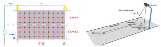
Figure 1.
Normative grid points for road lighting calculations or measurements (on the left); angles of observation α, deviation β and incidence γ to characterize the photometry of the road surface (on the right).
The spacing of the points in the longitudinal and transverse directions shall be determined as follows:
- D = S/N in the longitudinal direction where D is the spacing between points in the longitudinal direction in meters and S is the spacing between luminaires in the same row in meters. N is the number of points in the longitudinal direction with N = 10 for S ≤ 30 m and N is the smallest integer giving D ≤ 3 m if S > 30 m.
- d = W/3 in the transverse direction where d is the spacing between points in the transverse direction in meters and W is the width of the lane in meters.
For luminance evaluation, the position of the observer (symbolized with a green smiley in Figure 1 on the left) is 1.5 m above the road surface and at 60 m ahead the field of the relevant area. In the transverse direction, the observer shall be positioned in the center of each lane in turn.
From these luminance values, the following photometric parameters are computed [9,29,32]:
- The average luminance is the arithmetic mean of the luminance at the grid points in the field of measurement;
- The overall uniformity is the ratio of the lowest luminance, occurring at any grid point in the field of measurement, to the average luminance;
- The longitudinal uniformity is the ratio of the lowest to the highest luminance on points in the longitudinal direction along the center line of the lane.
The reflection properties of the road surface are used for the computation of a lighting installation. The most characteristic parameter is the luminance coefficient q, which is the ratio between the luminance L in cd/m2, which the observer sees, and the illuminance E in lux which is incident on the surface (Equation (1)).
Since the 1980s, for practical reasons, the luminance coefficient was replaced by the reduced luminance coefficient r in cd/m2/lux (Equation (2)), which is derived from q and given for a combination of fixed lighting angles β and tan(γ) (see Figure 1 on the right).
The standardized viewing height is again 1.5 m and the angle of observation α is constant at 1°, corresponding to an observation distance of 86 m.
To simplify the calculation, two indicators are defined by the CIE [13]. The average luminance coefficient Q0 represents the degree of lightness of the measured surface. It is computed as the average of the luminance coefficients over the specified solid angle Ω0, which only depends on β and γ values (Equation (3)). Q0 values given in this article were calculated directly by solving the double integral on β and γ using the trapezoidal rule.
The specular factor S1 represents the degree of specularity (shininess) of the observed surface. It is defined as the ratio between the reduced luminance coefficients of two specific illumination conditions (Equation (4)).
The figure and explanation proposed in [37] provide an original understanding of what S1 represents (see Figure 2). It can indeed be considered as the degree to which the surface at point P reflects more light from luminaire B, compared to that of luminaire A (h is the mounting height of a luminaire).

Figure 2.
Geometry used for the definition of the specularity factor S1 (inspired by [37]).
In CIE 144:2001, a classification system groups different surfaces according to the value of the specular factor S1 (see Table 1). Surfaces within a class are represented by a predefined r-table as well as values of Q0 and S1. The r-table can be rescaled if the real Q0 is known.

Table 1.
R classification from CIE 144:2001.
2.2. Ecl_R
Ecl_R is a road lighting calculations engine developed by the Cerema. Its development was motivated by the objectives of this study. With this software, it is possible to conduct classic lighting design and also to integrate the complete photometric characteristics of a pavement considering its heterogeneity and several observation angles. The instructions of CIE publication 140:2019 [9] have been carefully followed in the development of Ecl_R.
The possibilities of Ecl_R are the following:
- Classic lighting design: calculation of the photometric quantities representative of the performances of a lighting installation, using the standard CIE r-tables with or without Q0-scaling;
- Advanced lighting design: calculations with measured r-tables;
- Implementation of the concept of the moving observer: lighting calculations with a moving observer;
- Consideration of the road photometric heterogeneity: lighting calculations with r-tables measured at different points of the grid;
- Consideration of the new needs of road lighting: lighting calculations with r-tables measured at different observation angles.
Other possibilities, such as the visibility level calculation [43,44], are also available, but are not used in this study and are therefore not presented in detail.
In Annex B of CIE 140:2019, a set of test data and results benchmark values are provided to verify calculated values of road lighting computer programs. It was thus possible to validate the first functionalities of Ecl_R (see Appendix A). The following, calculations with r-tables measured on each point of the normative grid or with r-tables measured at different observation angles, are research tools and will be presented in the result part of this document.
2.3. Experimental Site
The data used in this study were obtained from the LUMIROUTE® experiment. The objective of LUMIROUTE® [17] was to assess an optimized, evolving pavement and lighting combination. To assess this, two conventional designed sections were compared with two LUMIROUTE® sections. On-site measurements of road photometry, luminance and power consumption were conducted every six months for three years.
The experimental site is a 2 × 2 lanes pavement 6.50 m wide and 400 m long, located on a suburban road in Limoges, France. The speed limit is 70 km/h with traffic between 150 and 300 trucks per day. The 4.25 m wide central reserve is equipped with a 9 m high lighting system with twin central arrangement. The entire road surface is a very thin asphalt concrete with a 0/10 mm gradation. The experimental zone consists of two sections of 200 m on either side of the boulevard (Figure 3). Sections 1 and 2 are the innovative sections called LUMIROUTE® sections. Sections 3 and 4 are ordinary “control sections”. Sections 1 and 4 are raw sections while the surfaces of Sections 2 and 3 have been treated with a high-pressure water jet to remove the thin bituminous layer from the surface. For the “control sections” Sections 3 and 4 composed of ordinary road surfaces and lighting, the lighting chosen was a metal halide (MH) discharge source. The two LUMIROUTE® sections were composed of lighter surfaces and adjustable LED lamps.
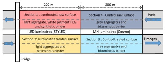
Figure 3.
Framework of the implementation of the four sections.
The resulting four combinations of road surface and lighting are summarized below:
- Section 1 is composed of the LUMIROUTE® 1 pavement (raw surface with light-colored aggregates, a synthetic binder and white pigment TiO2) combined with an LED illumination of 77 W (STYLED lamp, color temperature 4000 K);
- Section 2 consists of the LUMIROUTE® 2 pavement (water jet scrubbed pavement with light aggregates and a bituminous binder) combined with an LED illumination of 103 W (STYLED lamp, color temperature 4000 K);
- Section 3 is composed of a “Control treated” road surface (water jet scrubbed pavement with grey aggregate and a bituminous binder) combined with traditional lighting consisting of a 140 W MH discharge source (COSMO lamp, color temperature of 2811 K);
- Section 4 is composed of a “Control raw” road surface (current pavement with grey aggregate and a bituminous binder) combined with the same 140 W MH discharge source.
To simplify the reading, we will later on only mention pavements 1 to 4, offering the possibility for the reader to refer to the previous description.
2.4. Experimental Measurements and Devices
2.4.1. On-Site Measurement of Road Photometry
To study the spatial heterogeneity of pavement reflection properties, photometric evaluation was performed on-site with a portable measurement device named COLUROUTE [27,36] (picture on the left in Figure 4), which complies with the specifications of the CIE [13]. The luminance coefficients of the road surface are measured on-site, in daylight, and without sampling. COLUROUTE is equipped with a sensor directed at the measurement surface with an observation angle of 1° and has 27 sources set to successively illuminate this surface with different combinations of β and γ angles. These angles have been chosen in order to allow for the direct computation of the specularity factor S1 and to reconstruct by interpolation the complete r-table of the road surface. Calibration is performed on-site using reference plates measured with the Cerema laboratory gonioreflectometer [24,27]. The COLUROUTE outputs comprise the reduced luminance coefficient table (r-table), the average luminance coefficient Q0, and the specularity factor S1.
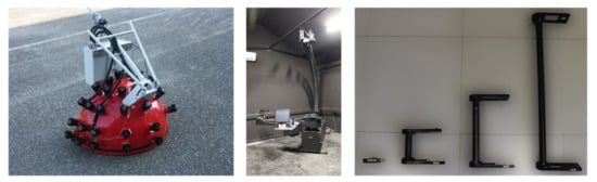
Figure 4.
The COLUROUTE device (on the left), the laboratory gonioreflectometer (in the middle) and ILMD supports for measurement at 2.29°, 10°, 20° and 45° (on the right).
2.4.2. Description of the Laboratory Gonioreflectometer
To study the influence of the observation angle on pavement reflection properties, photometric evaluation was performed in the laboratory with the Cerema gonioreflectometer [24,27]. It measures the reflection of road surfaces under the observation conditions of a motorist at an observation angle of 1° but also at other observation angles: 2.29°, 5°, 10°, 20° and 45°. It gives the 580 reflected luminance coefficients q(β,γ) of the r-table. The mechanical positioning unit consists of a steel base on which is adapted a rotating measuring arm to change the sight angle β from 0 to 180° and a light source positioning system to vary the angle of the incidence of light γ from 0° to 90° (see picture in the middle in Figure 4). The mechanical movement system of the lamp and the arm carrying the photometer is computer controlled, so the data acquisition is fully automated. The reference source is a type A halogen lamp with a color temperature of 2700 K (warm light) and an angle of diffusion of 10°. The light source is mounted on a metal arc with a radius of 2.05 m, whose movement corresponding to the incidence angle is ensured by a motor connected to an indexer-transformer, and the angle γ varies for its 29 positions. The illuminated area is a 10 × 10 cm square, always at the center of the sample. The “sample holder device” consists of a turntable allowing for the adjustment of the height of the sample, its lateral positioning, and the inclination to obtain the horizontality of the sample upper surface. This allows the measurement area to be centered on the sample without having to change the luminance sensor and source settings. The luminance sensor is an imaging luminance measuring device (ILMD) and is fixed on an articulated arm, made of light alloy, that is driven by a gear motor for the 20 positions of β from 0° to 180°. To change the observation angle, different supports (pictured on the right in Figure 4) for the ILMD have been designed during the SURFACE project [45].
2.4.3. On-Site Luminance Measurement
For the study of spatial heterogeneity, calculations from the COLUROUTE measurements were compared with average luminance and uniformities obtained from the luminance measurements. For on-site luminance measurements, Cerema has developed an automatic mobile system for measuring road lighting performance [28,46,47]. This device called CYCLOPE is an ILMD installed in a vehicle at a height of 1.5 m to comply with the standard. The normative measurement grid (Figure 1 on the left) is projected onto the luminance images [46]. For grid points positioning in these images, a model associating a distance to each line of the image is computed. Assuming a locally flat road between the vehicle and the measurement area, the pinhole model for the camera is used. In the longitudinal direction, the pinhole model allows for determining the rows in the image that correspond to the limits of the measurement area (please refer to the horizontal black lines in Figure 5 on the left). In the transverse direction, the road markings equations, computed by using road marking detection and robust fitting, delimit each lane (please refer to the red curves in Figure 5 on the left). Thus, a region of interest (ROI) is extracted from the image, which matches the field of luminance measurement for the relevant area. The last step is to calculate the positions of best pixels in the ROI that correspond to the grid points (please refer to the green points in Figure 5 on the left). The angular subtense of the measured road surface at each grid point shall not be greater than 2 arcmins in the vertical plane and not greater than 20 arcmins in the horizontal plane [42]. Since each pixel of the CYCLOPE camera has an angular aperture of 2 × 2 arcmins, the final luminance value at each grid point is calculated by taking the mean of 10 pixels in a transverse direction and 1 pixel in a longitudinal direction. An example of the resulting luminance values on the normative measurement grid is given on the right of Figure 5.
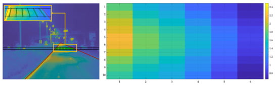
Figure 5.
On the left, example of luminance image recorded with CYCLOPE on pavement 1 with an observer placed in lane 1. The positions of the measurement grid points are displayed in green, the detected road marking lines in red and the horizontal black lines correspond to the standard observation distance 60 m and 89 m (luminaires are 29 m apart). On the right, representation of the resulting luminance values on the normative measurement grid.
From these luminance values, average luminance, overall uniformity, and longitudinal uniformity are computed according to the standardization [29]. The CYCLOPE measurements are traditionally operated in a moving vehicle. Dynamic measurement systems are mentioned in guidelines [42] and standards [32]. However, to limit some uncertainty factors in the study presented here, we performed static measurements for each section and each lane per section by mounting our ILMD outside the vehicle on a photographic stand in the standard geometry.
2.5. Methodology
2.5.1. New Metrics for Assessing the Link between Pavement Reflection Properties Deviations and Lighting Performance Criteria Deviations
The main objective of this study is to compare road lighting calculations with each other and to determine which ones give results as close as possible to values obtained from luminance measurements. Obviously, differences between values of average luminance and uniformities depend on how the pavement reflection properties have been treated in the calculations. To our knowledge, the CIE publications [8,9] or standardization [29,32], do not specify a hierarchy in the performance criteria of a lighting installation. Thus, in order to evaluate the differences between values calculated with two different r-tables, i and j, or between calculated and measured values, the average luminance, the overall uniformity, and the longitudinal uniformity should be considered simultaneously. For this reason, a global approach integrating the three photometric quantities and all the traffic lanes is proposed here, and a root mean squared deviation (RMSD) is calculated as follows:
where , and are average luminance, overall uniformity and longitudinal uniformity, respectively, in the considerate lane for r-table i; , and are average luminance, overall uniformity and longitudinal uniformity, respectively, in the considerate lane for r-table j; is a reference luminance (for to be a dimensionless quantity); , and are weighting factors and is the number of lanes. In this study, we have considered that was the average luminance to be maintained for the lighting class corresponding to our experimental site (class M3 [8,10]; average luminance equal to 1 cd/m2). The weighting factors , and are also fixed to 1. Equation (5) is thus a generalization of our first proposal in [48].
The same formula can obviously be used to compare calculations and measurements. In this case, it is sufficient to replace , and with values from measurements.
Considering our objectives, the relevance of will be established if this metric is representative of differences between pavement reflection properties. For this purpose, two new metrics for comparing two measurements of pavement photometry are also proposed, one based on Q0 and S1, the other on all values of the r-tables. The first one is also a root mean squared deviation, defined as follows:
where and are Q0 and S1, respectively, which are values calculated from r-table i; and are Q0 and S1, respectively, which are values calculated from r-table j. in this expression allows to be also a dimensionless quantity. It consists in dividing by a Q0ref (a reference Q0), here the Q0 of a perfect diffuser with a reflectivity equal to 1. This factor is an evolution since our first proposal [48], allowing for the set of metrics to be dimensionless and thus making their comparison mathematically cleaner.
Defining a metric based on Q0 and S1 values seems quite logical. Indeed, it is always these quantities that are investigated in studies comparing pavements, or that are interested in the evolution of pavement properties with ageing [17], or that consider their surface state [21,49,50].
The second metric considers a calculation of difference between pavements based on all available values in an r-table. A normalized root mean square deviation (NRMSD) calculation was therefore implemented (Equation (7)) where the averages of the r-tables’ values acts as a normalization factor.
where is the value of the r-table i for the position βk and tan(γ)l with k = [1:20] and l = [1:29]; is the value of the r-table j for the position βk and tan(γ)l.
These three metrics (, and ) have been used to assess the impact of pavement reflection properties deviations on lighting performance criteria deviations.
2.5.2. Experimental Measurements
To study the influence of pavement heterogeneity and of the observation angle, several experimental measurements were conducted, both on-site and in the laboratory.
At the LUMIROUTE® site, a specific experimental campaign was carried out to study the impact of the spatial heterogeneity of a pavement on lighting calculations when the pavements were 18 months old. Usually, with portable devices, six to ten measurements are made on-site [38,39,40]. In our case, the photometry of the four pavements in place was characterized with COLUROUTE and thirty r-tables were measured for each pavement. The location of the measurements has been chosen according to the CIE grid points, as shown on the left of Figure 6. Ten measurements were done in central tracks (points in rows B and E) and twenty in wheel tracks (other points).
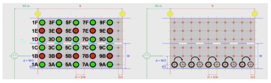
Figure 6.
On the left, repartition of r-table measurements to study spatial pavement reflection properties heterogeneity corresponding to half of the CIE grid points. Red circles correspond to measurements in central tracks, green circles to measurements in wheel tracks. On the right, principle of nearest neighbor selection for the grid points without measured r-table.
In parallel, the CYCLOPE measurements were carried out on the four pavements, thus providing experimental values of average luminance and uniformities to be compared with the calculations made from COLUROUTE measurements.
To study the influence of the observation angle, measurements for α (see Figure 1 on the right) equal to 1°, 2.29°, 5°, 10°, 20° and 45°, have been performed with the Cerema gonioreflectometer on pavement samples taken on the wheel track from the four sections of the LUMIROUTE® experimental site. We choose to use samples of the brand-new pavements collected during the first evaluation (T0) of the experiment. Generally, the pavements have the most different reflection properties in their new state [16] and the same tendency has been found for LUMIROUTE® pavements [17].
2.5.3. Lighting Calculations with Ecl_R
From all these measurements, different lighting calculations were carried out with Ecl_R, to study both the heterogeneity of the pavements and the influence of the observation angle.
The parameters used for the lighting calculations are presented in Table 2. They correspond to the settings of the lighting installations in place during the evaluation campaign of the LUMIROUTE® experiment at T18.
Table 2.
Lighting installations parameters used for calculations with Ecl_R.
First, Q0 and S1 values were calculated for the thirty measurements made on the grid. The thirty Q0 and the thirty S1 are then averaged to establish which would be the closest typical CIE pavement (see Table 1) and what scaling factor could be used for Q0.
Then, for the four pavements, different lighting calculations were performed with Ecl_R by varying the photometry of the pavement, considered as follows:
- A calculation using the standard r-table corresponding to the class of the pavement established from the thirty measurements;
- A calculation using the standard r-table scaled with the average of thirty Q0;
- Ten calculations using the ten r-tables measured on the central tracks;
- Twenty calculations using the twenty r-tables measured on the central tracks;
- A complete calculation using a dedicated r-table for each grid point. For the grid points where we did not directly have a measured r-table, we used the nearest neighbor according to the principle illustrated in Figure 6 (on the right).
In order to find out how many measurements are really needed to be representative of the heterogeneity of a pavement, additional calculations were made, considering different combinations of measured r-tables.
The influence of the observation angle on lighting calculations was also studied with Ecl_R. Seven calculations were carried out for each pavement: the first one, classical, using the r-table at 1° and a fixed observer, then six others with the r-tables associated with the different observation angles using a moving observer.
3. Results and Discussions
3.1. Spatial Heterogeneity Study
3.1.1. Analysis of Experimental Measurements
When the four pavements where 18 months old, thirty r-tables measurements (ten in the central tracks and twenty in the wheel tracks) were conducted with the COLUROUTE device on the CIE grid. All of the corresponding Q0 and S1 are represented in the Figure 7, and Table 3 gives the associated numerical values.
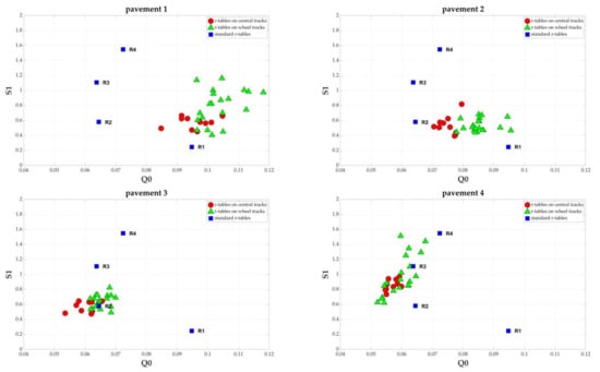
Figure 7.
Measurements of Q0 and S1 of the four pavements with one graph for each pavement. Red disks are used for the r-tables measured on central tracks, green triangles for the r-tables measured on wheel tracks and blue squares for the CIE standard r-tables.
Table 3.
Photometric characterization of the four pavements at T18 with the Q0 and S1 values.
According to the CIE classification (Table 1), pavements 1 to 3 are of type R2. Pavement 4 is of type R3. In Figure 7, except for pavement 3 where the measurements are well centered around the standard r-table, they are much further away for the three other pavements. In Table 3, the Q0 values for pavements 1 and 2 are higher than for pavements 3 and 4. This result was expected because these two pavements are innovative LUMIROUTE® light pavements. The specularity S1 is lower for pavements 2 and 3, as is the associated standard deviation. This is due to the water jet scrubbing treatment carried out on these pavements [17]. Concerning the differences between central tracks and wheel tracks, Q0 calculated from the measurements on the wheel tracks are systematically higher than Q0 calculated from the measurements on the central tracks. This is especially the case for the LUMIROUTE® light pavements. The same observations can be made for S1 values which are higher in the wheel tracks than in the central tracks for pavements 1, 3 and 4.
For each pavement, thirty lighting calculations were conducted, ten with r-tables measured on the central tracks and twenty with r-tables measured in the wheel tracks. Table 4 presents a summary of these calculations, giving for each photometric quantity the extreme values and associated amplitudes obtained in central tracks, in wheel tracks, and for the whole road. Each given value is the average of values obtained for the two lanes.
Table 4.
Summary of the thirty calculations conducted for the four pavements giving for each photometric quantity the extreme values (min and max) and associated amplitudes (Δ = max/min − 1 in %) obtained in central tracks (CT), in wheel tracks (WT) and for the whole road (CT + WT).
This table illustrates the variability of results depending on the r-table used, even if it belongs to the same pavement. Considering the values obtained for the whole road, the differences between minimal and maximal values are of the order of 20% for uniformities and 40% for the average luminance. Regarding differences between values obtained on the central tracks and on the wheel tracks, it seems to be very difficult to establish a general trend. The impact of pavement heterogeneity on the quality of a lighting installation is therefore clearly demonstrated. Our new metrics will be useful to investigate the link between the deviations of pavement reflection properties and the deviations of lighting performance criteria.
3.1.2. Implementation of the Proposed Metrics
To verify the relevance of the proposed metrics, we first examine the linearity between the values of Q0 and the average luminance, as well as between the values of S1 and the uniformities. Indeed, it was established in the 1970s [51,52] that the average luminance varied linearly with Q0 and that uniformities varied linearly with S1. Based on this principle, small differences between the values of Q0 and S1 should give small values of and vice versa.
Figure 8 shows the link between the thirty photometric measurements and the thirty associated lighting calculations for the four pavements. On the left is the average luminance as a function of Q0, in the middle the overall uniformity as a function of S1 and on the right the longitudinal uniformity as a function of S1. The correlation coefficients obtained for the different graphs are given in Table 5.
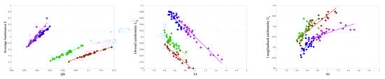
Figure 8.
On the left is the average luminance as a function of Q0, in the middle the overall uniformity as a function of S1 and on the right the longitudinal uniformity as a function of S1. Each given value is the average of values obtained for the two lanes. Red circles are associated with pavement 1, greens with pavement 2, blues with pavement 3 and magentas with pavement 4.
Table 5.
Correlation coefficients (R2) obtained between average luminance and Q0, overall uniformity and S1, longitudinal uniformity and S1 for the four pavements.
As in previous studies [51,52], very good correlations are obtained between the values of Q0 and the average luminance, and between the values of S1 and the overall uniformity. This is slightly less the case between S1 and longitudinal uniformity.
Given the correlations obtained (Table 5), the approach of simultaneously studying the variations of (Equation (5)), which represent lighting performance criteria deviations, with (Equation (6)), which represent pavement properties deviations, seems justified. and were therefore calculated by taking the r-tables two by two, i.e., 435 () possible combinations and therefore as many values for each proposed metric. 435 (Equation (7)) were also calculated using the same principle. Figure 9 plots for each pavement against on the left and against on the right. The corresponding correlation coefficients are given in Table 6.
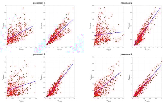
Figure 9.
For each pavement, variations of against on the left and against on the right.
Table 6.
Correlation coefficients (R2) between and and between and .
There are very good correlations between and as opposed to and . This means that which includes both Q0 and S1 is not sufficient to explain the variations in average luminance and uniformities taken simultaneously. On the other hand, considering the complete r-table with , differences in pavement reflection properties are immediately translated into differences in lighting calculations, regardless of the type of pavement or lighting installation.
This demonstrates that is a metric of comparison between lighting performance criteria that is representative of differences in pavement reflection properties.
3.1.3. Calculation of a Threshold on
For the next steps of our analyses, was used as a metric for comparison between lighting calculations and on-site luminance measurements. Based on linear regressions shown in Figure 9 and the associated correlations (Table 6), we can deduce that the smaller the value of , the smaller the value of , and the better r-table used in the calculation will tend to represent the properties of the pavement included in luminance measurements. A question then arises. For what values of can we consider that the average luminance and uniformities obtained from a lighting calculation are similar to those obtained from the on-site luminance measurements and that, in this case, the r-table used in the calculation is representative of the actual pavement reflection properties? To address this question, it seems necessary to establish a threshold value of (denoted ), below which it will be considered that calculations and measurements provide similar results.
In this study, the on-site luminance measurements are considered as the reference. The relative measurement uncertainty associated with the CYCLOPE system used in static configuration and in outdoor conditions was estimated to be 13.5% with a coverage factor of two. To establish the value of , this uncertainty was introduced into the calculation of in order to study the amplitude of the variation of as a function of the measured luminances and their associated uncertainty. The Monte Carlo method was used following the instructions of the Supplement 1 to the “Guide to the expression of uncertainty in measurement” (GUM) [53].
For each pavement, sixty luminance measurements on the normative grid points are available for an observer located in lane 1 and sixty luminance measurements are also available for an observer located in lane 2. Table 7 gives an example of the measurements made for the pavement 1.
Table 7.
Luminance measurements (in cd/m2) for the pavement 1 with an observer located in lane 1 (values on the left) and in lane 2 (values on the right). Values in bold correspond to coordinates on the normative grid.
From these sixty measurements, the average luminance, general uniformity, and longitudinal uniformity are calculated for each observer position. Table 8 presents a summary of the CYCLOPE measurements for the four pavements. These results are therefore the reference values in the various calculations of .
Table 8.
Average luminance (in cd/m2), overall uniformity, and longitudinal uniformity obtained from CYCLOPE measurements for the four pavements.
To evaluate the impact of the measurement uncertainty associated with the CYCLOPE device in the calculation of , the following approach was taken. It was considered that if the luminance measurements had been made a very large number of times, then, at each point of the grid, these measurements would have been statistically distributed according to a normal distribution, centered on the value effectively measured and with a standard deviation equal to half the measurement uncertainty of the reference instrument. Figure 10 illustrates this principle by simulating the case where the measurements were made one million times, using the values measured for pavement 1 and an observer placed in lane 1 (Table 7 on the left).
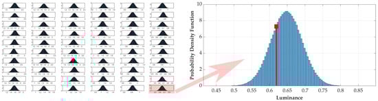
Figure 10.
On the left, construction of the normal statistical distributions of luminance at each point of the measurement grid for pavement 1 and an observer located in lane 1. On the right, focus on one of these statistical distributions and illustration of the principle of random luminance value selection (red square).
In the Monte Carlo method implemented, the principle consists of randomly taking a simulated luminance value for each point of the grid respecting the statistical distribution associated with the measurement uncertainty of the reference (Figure 10 on the right). New values of the average luminance and uniformities are then calculated and the between these simulated values and the reference values can be evaluated. This process was repeated one million times, as recommended in Supplement 1 of the GUM. Figure 11 provides the statistical distributions of the obtained for the four pavements.
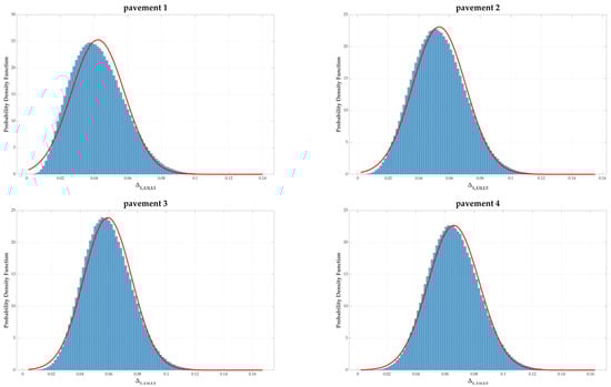
Figure 11.
Statistical distributions of the obtained for the four pavements (blue bars) and associated normal distributions (red curves).
It was verified by performing a Kolmogorov-Smirnov test [54] that each distribution of followed a normal distribution. This assumption is also verified graphically in Figure 11 where the red curves represent the normal distributions obtained from the averages and the standard deviations (see values in Table 9) calculated on the distributions of .
Table 9.
Summary of averages, standard deviations, and thresholds calculated from distributions of for the four pavements.
Since the normality assumption is verified, it is possible to look at the range of variation of the values of using their average extended by plus or minus three times the standard deviation from this average. This range covers 99.73% of the possible values of resulting from the uncertainty of the reference instrument. In the end, the threshold value corresponds to the maximum value of this range. Table 9 summarizes all of these calculations for the four pavements.
Subsequently, when the values of the average luminance and uniformities obtained from a lighting calculation will be compared with those obtained from reference measurements, it will be considered that these values are similar if is less than the associated with the studied pavement. This is a strong requirement. It means that a lighting calculation based on input data (luminaires, road surface and geometry, etc.), each with its own uncertainty, must provide a deviation from the reference within the range of variation of the deviations associated with the uncertainty of the reference alone. In other words, the deviation between the calculation and the reference measurements should be of the order of the deviation which would have been obtained from two consecutive measurements.
Because of the correlations established between and (Table 6), it will also be assumed that the r-table used in the lighting calculation is representative of the actual optical properties of the studied pavement.
3.1.4. Analysis of the Calculations
Table 10 shows the main results obtained from all the calculations carried out for each pavement. Average luminance, overall uniformity and longitudinal uniformity are given for each lane. between lighting calculation and luminance measurements, is provided in the last column. The reported lighting calculations are as follows:
Table 10.
Calculation results for different ways of integrating the optical properties of pavements. Calculations that meet the requirement () are highlighted in bold.
- Calculation with the standard r-table;
- Calculation with the standard r-table Q0-scaled using the values from Table 3;
- Calculations with the r-tables measured in central tracks which give the minimum and the maximum values among the ten calculations performed;
- Calculations with the r-tables measured in wheel tracks which give the minimum and the maximum values among the twenty calculations performed;
- Complete calculation using a dedicated r-table for each point of the grid.
Looking at the different obtained for each pavement and comparing them with the thresholds provided in Table 9, the calculations performed with the standard r-table do not meet the requirement for three out of four pavements. This is also the case for the calculations performed with the scaled r-tables based on Q0 values. These results confirm that the use of standard r-tables, scaled or not, is a hazardous exercise.
In contrast, in the case of calculations based on measured r-tables, there is always at least one central track measurement and one wheel track measurement for each pavement that meets the requirement. The complete calculations also systematically comply with the requirement. Among the calculations performed with measured r-tables, it was expected that the complete calculations would always show the lowest deviations. Indeed, the methodology associated with the complete calculation is the one that seems most likely to integrate the pavement heterogeneity. This assumption is true for pavements 1 and 4, whereas for pavements 2 and 3, an r-table measured in the wheel track offers the smallest deviation. For pavements 1 and 4, the deviations obtained with the complete calculation are very close to those obtained with the best measurement in the central track or in the wheel track. Whereas for pavements 2 and 3, the deviations associated with the best measurement in the wheel track are significantly lower than those obtained with the complete calculation. This demonstrates that the measurement methodology associated with the complete calculation is neither mandatory nor the most relevant to take into account for the pavement heterogeneity in a lighting calculation. This result is really important because the thirty measurements method is time-consuming and not compatible with operational constraints.
3.1.5. Implications for On-Site Measurements Methodology
In absolute terms, the use of a single measured r-table for the lighting calculation is sufficient to meet the requirements. However, this “optimal” r-table can be located in the central track as well as in the wheel track, and among all the measurements carried out in this study, it was never in the same place on the road. In addition, there are also measured r-tables that do not comply with the requirement, showing deviations that are sometimes greater than those obtained with the standard r-tables. It is therefore necessary to adopt a methodology for on-site measurements that can guarantee representative data for the surface to be illuminated.
Different scenarios are considered, deliberately leaving aside the notion of the operator’s expertise. These expertise may vary from one individual to another, and is based on the subjective criteria of the visual representativeness of the area to be measured. Our aim is to provide methodological guidelines that can be used by a standard operator.
- The first scenario consists of making a naive measurement, i.e., completely at random. It was therefore examined, for each pavement, how many of the thirty calculations made from the thirty available r-tables met the requirement.
- The second scenario is to make a single central track measurement. For each pavement, the number of calculations that met the requirement was examined from among the ten calculations made from the ten available r-tables in the central tracks.
- The third scenario is to make a single wheel track measurement. For each pavement, the number of calculations that met the requirement was examined from the twenty calculations made from the twenty available r-tables in the wheel tracks.
- The fourth scenario is to make one measurement in the central tracks and one in the wheel tracks. Additional calculations were made with Ecl_R to test the 200 () possible combinations. The r-table used in each calculation is the average of the selected central track r-table and the selected wheel track r-table. It was then examined for each pavement how many of these calculations met the requirement out of the 200 performed.
- The fifth scenario is to make two measurements in the central tracks and two in the wheel tracks. New calculations were performed to test 8550 () possible combinations. The r-table used in each calculation is the average of the four selected r-tables. It was then examined for each pavement how many of these calculations met the requirement out of the 8550 performed.
- The sixth scenario is to make three measurements in the central tracks and three in the wheel tracks. New calculations were performed to test 136,800 () possible combinations. The r-table used in each calculation is the average of the six selected r-tables. It was then examined, for each pavement, how many of the 136,800 calculations met the requirement.
Table 11 gives, for each pavement, the percentage of confidence associated with each scenario.
Table 11.
Confidence percentages associated with the different measurement scenarios (CT: r-table measured in central tracks; WT: r-table measured in wheel tracks).
In accordance with practice [17,38,39,40], the measurement methodology which takes into account the pavement heterogeneity consists of making measurements in both the central track and the wheel track. Four measurements (Scenario 5) already offer a very interesting level of confidence. Six measurements (Scenario 6), positioned in a completely arbitrary manner, without any notion of operator expertise, allow to systematically exceed 85% of confidence in the ability of the resulting r-table to reflect the actual pavement reflection properties. This result seems to us very satisfactory and scientifically confirms previous measurement practices. The process of averaging several r-tables to obtain a single resulting r-table was also not common prior to this study. Our results show that this approach can be robust. Furthermore, the advantage of using this single resulting r-table is that the exercise of lighting design is not more expensive in terms of time and computation than using a standard r-table. The constraint consists in carrying out measurements in the field. However, since the number of required measurements is moderate, the operational constraints remain manageable, particularly with regards to the potential energy savings made by taking into account the actual properties of the pavement [17].
The presented methodology and previous results have demonstrated that our proposed metrics are useful for the optimization of lighting design. To go further, these metrics were also tested for other observation angles. As public lighting is often urban, it is important to better integrate the different uses of urban spaces at night and to design lighting better adapted to the real needs of users.
3.2. Influence of Observation Angle on Pavement Reflection Properties
3.2.1. Analysis of Experimental Measurements
For the four pavements, measurements for the observation angles of 1°, 2.29°, 5°, 10°, 20° and 45° have been performed with Cerema gonioreflectometer. We chose to use T0 samples because it was in the new state that the four pavements showed the most different reflection properties [15,17]. Q0 and S1 values associated with these different measurements have been calculated (Table 12). Although it is not mentioned in the reference documents [13] that these factors can be used for other observation angles, there is nothing in their mathematical expression (Equations (3) and (4)) that prohibits this, since they depend only on the β and γ angles (Figure 1 on the right).
Table 12.
Photometric characterization of the four pavements at different observation angles with the Q0 and S1 values.
Figure 12 provides a graphical representation of the photometric coefficients Q0 and S1 for the different observation angles. The photometric solids associated with these r-tables are drawn in Figure 13. They are a 2D projection of r-table values, and the horizontal axis is 104.r.sinγcosβ, while the vertical axis is 104.r.cosγ.
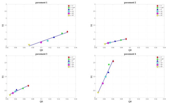
Figure 12.
Measurements of Q0 and S1 of the four pavements at different observation angles with one graph for each pavement.
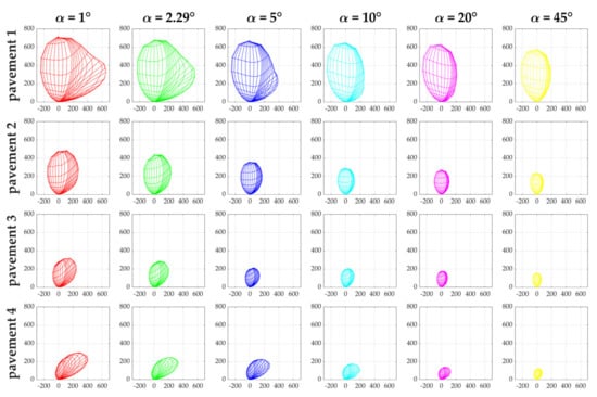
Figure 13.
Photometric solids for the four pavements at different observation angles.
Looking at Table 12 and Figure 12, the same trend for all four pavements can be noted, namely the decrease in Q0 and S1 values as the observation angle α increases. These observations are in line with those produced in previous studies [44]. It can even be underlined that these decreases seem to be linear with each other, considering the calculated correlation coefficients (please refer to the last line of Table 12). The same observations are made from the photometric solids in Figure 13. The decrease in the area covered by the 2D projection is directly related to the decrease in Q0 values. The decrease in S1 is reflected in the tendency of the solids to become more and more spherical as the observation angle of the observation increases. This reflects an increasingly diffuse behavior [44].
3.2.2. Analysis of the Calculations
From these six r-tables per pavement, seven lighting calculations were performed with Ecl_R, using the parameters given in Table 2. The first was carried out conventionally using the r-table measured at 1° and a fixed observer. Then, six other calculations were performed with r-tables measured at the different observation angles and a moving observer. Table 13 shows all the results obtained.
Table 13.
Calculation results for different observation angles.
For all the pavements, a clear and continuous decrease in average luminance is systematically observed when the observation angle increases. From 1° to 2.29°, the luminance decreases by 7% for pavement 1 and by about 15% for pavements 2, 3 and 4. This demonstrates the important effect of the observation angle in the design of a lighting installation.
This decrease can also be observed for the longitudinal uniformity for pavements 1 to 3, though less so for pavement 4. It is difficult to identify a general trend for the overall uniformities, which seem to be less sensitive to the change of angle.
These trends already observed for on-site luminance measurements [28,55] are here confirmed with the calculations. All these elements show the interest of using a moving observer, when we are interested in the effect of the observation angle on lighting performance criteria.
3.2.3. Implementation of the Proposed Metrics
In order to evaluate the relevance of in the case of the evolution of pavement reflection properties with the observation angle, the same approach as for the study of heterogeneity was reproduced. The variations of were studied as a function of the deviations in the values of Q0 and S1 represented by . For this purpose, the linearities between the values of Q0 and the average luminance as well as between the values of S1 and uniformities were examined. A graphical representation (Figure 14) of these variations and the correlation coefficients obtained (Table 14) are shown below.
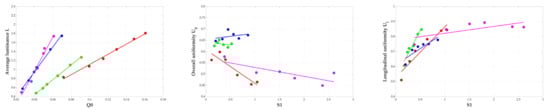
Figure 14.
On the left is the average luminance as a function of Q0, in the middle the overall uniformity as a function of S1 and on the right the longitudinal uniformity as a function of S1. Each given value is the average of values obtained for the two lanes. Red circles are associated with pavement 1, green with pavement 2, blue with pavement 3 and magenta with pavement 4.
Table 14.
Correlation coefficients (R2) obtained between average luminance and Q0, overall uniformity and S1, longitudinal uniformity and S1 for the four pavements.
Excellent correlations between Q0 and the average luminance values are obtained. Good correlations between S1 and longitudinal uniformity also exist, especially for the first three pavements. The results are more difficult to interpret between S1 and the overall uniformity for which the variation according to the observation angle is not obvious. This is in line with the first interpretations of results presented in Table 13. Nevertheless, examining jointly the variations of and again seems justified. These two quantities were calculated by taking the r-tables two by two, i.e., 15 () possible combinations. was also evaluated. The results for the four pavements are given in Figure 15 together with the associated correlation coefficients (Table 15).
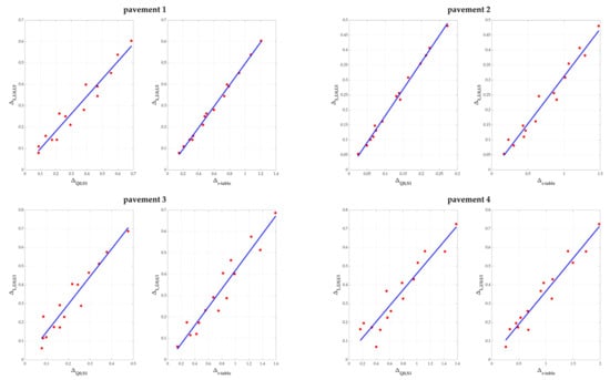
Figure 15.
For each pavement, variations of against on the left and against on the right.
Table 15.
Correlation coefficients (R2) between and and between and .
Excellent correlations between and , and between and are obtained. For , associating these results with those obtained previously, it clearly becomes a privileged metric for expressing differences between pavement reflection properties. As for , even if the correlations between luminance and Q0, and between uniformities and S1, are of the order of those obtained in the study on spatial heterogeneity, it must be noted that, for a variable observation angle, can also be used to predict deviations in lighting calculations. We attribute this result to the amplitude of the variations of the values of Q0 and S1 and of the values of luminance and uniformities when the observation angle increases. Indeed, these amplitudes are much larger than in the spatial heterogeneity study, due to the evolution from specular to diffuse pavement behavior. is a metric capable of reflecting this evolution. The linearities observed in Figure 12 confirm this. These results also confirm the implementation and relevance of moving observation in lighting calculations because the average luminance and uniformities obtained directly reflect the evolution of Q0 and S1.
Concerning , it is confirmed that it is indeed a significant metric in lighting calculations with different pavement reflection properties, this time in the case of the variation of the observation angle. Therefore, in Table 16, have been calculated from values of Table 13, taking as reference the calculation at 1° for a fixed observer. Not surprisingly, the smallest deviations are obtained for the 1° calculations with a moving observer, and then increased continuously up to the 45° angle.
Table 16.
Calculations of and for the four pavements. The r-table measured at 1° is considered as the reference for calculations. The values of average luminance and uniformities obtained at 1° for a fixed observer (Table 13) are considered as the reference for calculations.
In Table 16, were also calculated for each angle, taking the r-table at 1° as a reference.
It then seemed interesting to plot the variations of these and as a function of the observation angle (Figure 16).
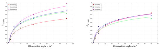
Figure 16.
Variations of (at left) and (at right) as function of the observation angle for the four pavements.
For all four pavements, a logarithmic increase of and is observed as a function of the observation angle. This illustrates once again the evolution of the pavements towards a more and more diffusive behavior when the observation angle increases. Indeed, we see equally large variations between 1° and 10° as between 10° and 45° with a stabilization of the pavement reflection properties reflected by the convergence of and . For the we also observe that the calculation points and the logarithmic regressions are relatively close, even if the optical properties of the pavements are basically very different. This would argue for a relatively systematic evolution of as a function of the observation angle, regardless of what the pavement formulation is and whether a surface treatment is performed.
4. Conclusions and Perspectives
This paper presents a new metric (called ) able to compare the performance of a lighting installation with a single value related both to the average luminance, and the overall and longitudinal uniformities when pavement reflection properties are variable. Two metrics able to evaluate the differences between different r-tables are also proposed. It was found that , the root mean square deviation between values of average luminance and uniformities from calculations with two different r-tables, was representative of the normalized root mean square deviation between these two r-tables (called ). This result was obtained from measured values on four different pavements, in a study of the spatial heterogeneity of the optical properties of pavements. It was then confirmed in a study of the evolution of these properties with the observation angle. The normalized root mean square deviation is a new way of characterizing differences between pavements, rather than reasoning about Q0 and S1 alone because, according to our results, these two factors do not explain lighting calculation differences. Our proposed metrics and directly relate pavement reflection properties to the performance of a lighting installation with a correlation coefficient better than 0.9 in a large majority of cases.
According to previous work [17], the benefit of measuring pavement reflection properties when designing a lighting installation was confirmed in this study. In terms of measurement methodology, it was shown that performing r-table measurements on the central track and on the wheel track is necessary to take into account the pavement heterogeneity. From a large panel of pavement photometry measurements carried out on half of the CIE grid points, it was possible to investigate what the minimum number of measurements necessary to be representative of the photometry of a pavement in place was. We have shown that six measurements, three on central tracks and three on wheel tracks, are sufficient to determine an average r-table representative of the real pavement properties with a very good level of confidence.
All these results could be inputs for the CIE Technical Committee 4-50 [56] on road photometry, one of whose objectives is to revise CIE Publication 144.
Nevertheless, it still seems ambitious to assume that the on-site measurement of luminance and road photometry will be generalized. Despite the rapid and significant developments in the use of LEDs in urban lighting, designing practices are evolving more slowly. The use of luminance as a performance criterion is far from being systematic, and having the actual photometry of the pavement is therefore not a priority. The question of defining new standard r-tables is therefore legitimately raised. In the absence of measurements, they could limit the harmful effects of lighting (for example, energy waste and light pollution) by updating obsolete standards. The actual work of the French group “Pavements and Lighting” [24] aims to characterize the optical properties of different families of urban pavements. The database currently includes thirty-eight different pavements and photometric measurements were carried out on these pavements when new and after thirty months of natural ageing. These measurements were also conducted at two different observation angles, 1° and 10°. Thus, based on all these new measurements and the metrics introduced in this article, it could be envisaged to define new standard r-tables, which are more representative of current pavements, particularly for urban applications.
Finally, our investigations into the observation angle have shown a real influence of this angle on the pavement reflection properties and on the performance of a lighting installation. We thus find results previously produced in the laboratory [44] and from on-site luminance measurements [28,55]. Some of our observations of when the observation angle changes, such as the linear variations between those of Q0 and S1, or the logarithmic evolutions of and , suggest the possibility of predicting the evolution of pavement reflection properties as a function of the observation geometry. We will investigate this in future studies.
The interest of using a moving observer concept [31] was confirmed in this work. Its use for angles greater than 1° is a good way to report the impact of the observation angle on the performance of a lighting installation. We are aware that a moving observer who always looks at the same distance is not really representative of the spatial aspects of visual exploration during travel [57,58,59]. It is nonetheless relevant to one of the main reasons for lighting, namely to detect an obstacle at a sufficient distance to stop.
In the perspective of proposing new geometries adapted to urban uses and different types of users, the reduction in average luminance and uniformities when the angle increases will be a central issue. Especially since, as we have shown, this decrease is strong in the interval between 1° and 10° and we assume that it is in this interval that these new geometries will be proposed. It will therefore be necessary to revise the performance requirements of a lighting installation, mainly by reducing the average luminance level to be maintained. However, since it is a question of better considering urban uses and consequently reduced travel speeds, we believe that this reduction of average luminance will not be prejudicial in terms of visual comfort. It could even be a source of new possibilities for saving energy and reducing light pollution. To confirm this, we intend to reintegrate visibility calculations as a performance criterion for lighting installations in future works, as was already the case in previous recommendations [11,60].
Author Contributions
Conceptualization, F.G. and V.M.; methodology, F.G. and V.M.; software, F.G.; validation, F.G. and V.M.; formal analysis, F.G., V.M., V.B. and F.F.; investigation, F.G., V.M., V.B., L.L. and S.L.; resources, F.G., V.M., V.B., F.F. and S.L.; data curation, F.G., V.M. and S.L.; writing—original draft preparation, F.G.; writing—review and editing, V.M., V.B., F.F., L.L. and S.L.; visualization, F.G.; supervision, F.G. and V.M. All authors have read and agreed to the published version of the manuscript.
Funding
This research received no external funding.
Institutional Review Board Statement
Not applicable.
Informed Consent Statement
Not applicable.
Data Availability Statement
The data presented in this study are available on request from the corresponding author.
Acknowledgments
Authors acknowledge Aurélia Nicolaï from Spie batignolles malet, Alexandre Taron from Thorn and Jean-Luc Bicard from Cerema for their technical support. Authors are very grateful to Roland Brémond from Gustave-Eiffel University for his enlightening review.
Conflicts of Interest
The authors declare no conflict of interest.
Appendix A
Performances of Ecl_R software have been evaluated and validated using the CIE 140:2019 methodology. In Annex B of CIE 140:2019, a set of test data and results benchmark values are provided to verify calculated values of road lighting computer programs. Seven different classical lighting situations are defined with the corresponding installation parameters: spacing between luminaires, road width, number of lanes, mounting height, luminous intensity data, lighting arrangement, etc. The lighting computation on these seven profiles were conducted with both Ecl_R and DIALux® to use a software widely employed by lighting professionals. The aim was to have three different results and to be able to position Ecl_R in terms of uncertainties, because CIE 140:2019 does not provide any tolerance on the calculated values. Table A1 presents these comparisons for one particular situation with three lanes (situation 5). Table A2 gives the results for the six other situations.
Table A1.
Comparison of the results provided in CIE 140:2019, DIALux® and Ecl_R for the situation 5 with Lave (average luminance in cd/m2), U0 (overall uniformity), Ul (longitudinal uniformity), Lv (veiling luminance in cd/m2), TI (threshold increment), Eh (average horizontal illuminance in lux), Uh (uniformity of illuminance) and REI (edge illuminance ratio).
| Road Lighting Situation | CIE 140:2019 | DIALux® | Ecl_R | ||||||||||
|---|---|---|---|---|---|---|---|---|---|---|---|---|---|
| Fixed Observer | Moving Observer | ||||||||||||
| Lane 1 | Lane 2 | Lane 3 | Lane 1 | Lane 2 | Lane 3 | Lane 1 | Lane 2 | Lane 3 | Lane 1 | Lane 2 | Lane 3 | ||
| Situation 5 | Lave | 0.44 | 0.42 | 0.41 | 0.43 | 0.41 | 0.40 | 0.44 | 0.42 | 0.41 | 0.44 | 0.42 | 0.40 |
| U0 | 0.45 | 0.57 | 0.67 | 0.43 | 0.56 | 0.72 | 0.45 | 0.57 | 0.67 | 0.48 | 0.59 | 0.68 | |
| Ul | 0.79 | 0.71 | 0.75 | 0.79 | 0.72 | 0.73 | 0.79 | 0.73 | 0.75 | 0.79 | 0.73 | 0.75 | |
| Lv | 0.105 | 0.095 | 0.063 | - | - | - | 0.105 | 0.095 | 0.063 | 0.105 | 0.095 | 0.063 | |
| TI | 11.0 | 10.4 | 7.10 | 11 | 10 | 7 | 11.0 | 10.4 | 7.10 | 11.0 | 10.4 | 7.10 | |
| Eh | 7.00 | 7.04 | 7.04 | ||||||||||
| Uh | 0.28 | 0.27 | 0.28 | ||||||||||
| REI | 0.76 | - | 0.76 | ||||||||||
Looking at the differences between our results for a fixed observer (Table A1 and Table A2) and those presented in CIE 140:2019, 75% of our results are strictly equal to the values provided by CIE 140:2019, and all of them present differences lower than 5%. Compared to the results from DIALux®, we achieve superior performance in these situations. Thus, we consider that our software Ecl_R is valid for classic lighting design.
The second step was to introduce the concept of the moving observer [28,31] and evaluate its impact for the 1° geometry. We thus carried out the same calculations on the seven test situations, this time considering a moving observer. Table A1 and Table A2 offer a comparison between the reference values and the Ecl_R results for a fixed observer and for a moving observer.
Table A2.
Comparison of the results provided in CIE 140:2019, DIALux® and Ecl_R for the six other situations.
Table A2.
Comparison of the results provided in CIE 140:2019, DIALux® and Ecl_R for the six other situations.
| Road Lighting Situations | CIE 140:2019 | DIALux® | Ecl_R | ||||||
|---|---|---|---|---|---|---|---|---|---|
| Fixed Observer | Mobile Observer | ||||||||
| Lane 1 | Lane 2 | Lane 1 | Lane 2 | Lane 1 | Lane 2 | Lane 1 | Lane 2 | ||
| Situation 1 | Lave | 0.26 | 0.26 | 0.25 | 0.26 | 0.26 | 0.26 | 0.26 | 0.27 |
| U0 | 0.14 | 0.15 | 0.14 | 0.15 | 0.14 | 0.15 | 0.14 | 0.15 | |
| Ul | 0.56 | 0.64 | 0.55 | 0.68 | 0.56 | 0.64 | 0.56 | 0.64 | |
| Lv | 0.877 | 0.314 | - | - | 0.897 | 0.329 | 0.897 | 0.329 | |
| TI | 141 | 49.7 | 126 | 50 | 145 | 52.0 | 143 | 51.6 | |
| Eh | 2.50 | 2.54 | 2.52 | ||||||
| Uh | 0.28 | 0.28 | 0.28 | ||||||
| REI | 0.32 | - | 0.31 | ||||||
| Situation 2 | Lave | 0.26 | 0.26 | 0.26 | 0.26 | 0.26 | 0.26 | 0.26 | 0.26 |
| U0 | 0.35 | 0.32 | 0.31 | 0.32 | 0.35 | 0.32 | 0.37 | 0.37 | |
| Ul | 0.33 | 0.33 | 0.33 | 0.33 | 0.33 | 0.33 | 0.33 | 0.33 | |
| Lv | 0.636 | 0.626 | - | - | 0.653 | 0.644 | 0.653 | 0.644 | |
| TI | 101 | 99 | 95 | 95 | 104 | 102 | 103 | 102 | |
| Eh | 2.50 | 2.54 | 2.52 | ||||||
| Uh | 0.32 | 0.32 | 0.31 | ||||||
| REI | 0.47 | - | 0.46 | ||||||
| Situation 3 | Lave | 0.55 | 0.60 | 0.54 | 0.60 | 0.55 | 0.60 | 0.55 | 0.60 |
| U0 | 0.52 | 0.54 | 0.51 | 0.52 | 0.52 | 0.54 | 0.54 | 0.54 | |
| Ul | 0.68 | 0.70 | 0.67 | 0.68 | 0.68 | 0.70 | 0.68 | 0.70 | |
| Lv | 0.130 | 0.138 | - | - | 0.131 | 0.139 | 0.131 | 0.139 | |
| TI | 11.5 | 11.3 | 10 | 11 | 11.6 | 11.3 | 11.5 | 11.3 | |
| Eh | 7.80 | 7.85 | 7.77 | ||||||
| Uh | 0.34 | 0.33 | 0.34 | ||||||
| REI | 0.64 | - | 0.64 | ||||||
| Situation 4 | Lave | 0.88 | 0.87 | 0.87 | 0.86 | 0.88 | 0.87 | 0.87 | 0.87 |
| U0 | 0.54 | 0.51 | 0.52 | 0.50 | 0.54 | 0.51 | 0.53 | 0.53 | |
| Ul | 0.53 | 0.53 | 0.51 | 0.51 | 0.53 | 0.53 | 0.53 | 0.53 | |
| Lv | 0.228 | 0.227 | - | - | 0.228 | 0.228 | 0.228 | 0.228 | |
| TI | 13.8 | 13.8 | 13 | 13 | 13.8 | 13.9 | 13.9 | 13.8 | |
| Eh | 12.0 | 12.0 | 12.0 | ||||||
| Uh | 0.49 | 0.49 | 0.49 | ||||||
| REI | 0.61 | - | 0.61 | ||||||
| Situation 6 | Lave | 1.17 | 1.30 | 1.16 | 1.30 | 1.17 | 1.31 | 1.17 | 1.31 |
| U0 | 0.49 | 0.49 | 0.47 | 0.48 | 0.49 | 0.49 | 0.50 | 0.50 | |
| Ul | 0.62 | 0.72 | 0.61 | 0.69 | 0.62 | 0.72 | 0.62 | 0.72 | |
| Lv | 0.239 | 0.181 | - | - | 0.243 | 0.184 | 0.243 | 0.184 | |
| TI | 11.5 | 8.00 | 11 | 7 | 11.6 | 8.11 | 11.7 | 8.10 | |
| Eh | 16.2 | 16.0 | 16.2 | ||||||
| Uh | 0.50 | 0.50 | 0.50 | ||||||
| REI | 0.67 | - | 0.67 | ||||||
| Situation 7 | Lave | 0.53 | 0.58 | 0.53 | 0.58 | 0.53 | 0.58 | 0.53 | 0.59 |
| U0 | 0.45 | 0.46 | 0.44 | 0.46 | 0.45 | 0.46 | 0.46 | 0.47 | |
| Ul | 0.84 | 0.91 | 0.86 | 0.89 | 0.84 | 0.91 | 0.84 | 0.91 | |
| Lv | 0.173 | 0.127 | - | - | 0.173 | 0.127 | 0.173 | 0.127 | |
| TI | 15.6 | 10.6 | 15 | 10 | 15.6 | 10.6 | 15.6 | 10.6 | |
| Eh | 7.00 | 7.04 | 7.01 | ||||||
| Uh | 0.50 | 0.50 | 0.50 | ||||||
| REI | 0.62 | - | 0.62 | ||||||
The results obtained for a moving observer are very close to those obtained with a fixed observer. The most significant differences are observed for some overall uniformity calculations, probably due to variations in the minimum luminance on the grid. Nevertheless, we consider that the moving observer concept is valid for lighting calculations and can be used with other observation angles than the traditional 1°.
References
- Outdoor LED Lighting Market|Size, Growth, Trend and Forecast to 2023|Markets and Markets. Available online: https://www.marketsandmarkets.com/Market-Reports/outdoor-led-lighting-market-%20211822268.html (accessed on 11 July 2021).
- Kyba, C.; Kuester, T.; Sanchez de Miguel, A.; Baugh, K.; Jechow, A.; Hölker, F.; Bennie, J.; Elvidge, C.; Gaston, K.; Guanter, L. Artificially Lit Surface of Earth at Night Increasing in Radiance and Extent. Sci. Adv. 2017, 3, e1701528. [Google Scholar] [CrossRef] [PubMed] [Green Version]
- Tardieux, P.; Greffier, F.; Taron, A. Projet Lumiroute®: Évaluation Du Système EQflux®. RGRA 2017, 950, 18–21. [Google Scholar]
- Soardo, P.; Iacomussi, P.; Rossi, G. The Luminance Coefficient in Road Lighting. A Parameter to Save Energy and Reducing Atmospheric Pollution. In Proceedings of the 11th Lux Europa International Congress, Istanbul, Turkey, 9–11 September 2009. [Google Scholar]
- Sordello, R. Pollution lumineuse et trame verte et bleue: Vers une trame noire en France? Territ. Mouv. Rev. Géographie Aménagement Territ. Mov. J. Geogr. Plan. 2017. [Google Scholar] [CrossRef]
- Aménagement, Urbanisme, Biodiversité, Éclairage: Une Série de Fiches Pratiques Pour les Différents Acteurs. Available online: http://www.cerema.fr/fr/actualites/amenagement-urbanisme-biodiversite-eclairage-serie-fiches (accessed on 11 July 2021).
- Fotios, S.; Gibbons, R. Road Lighting Research for Drivers and Pedestrians: The Basis of Luminance and Illuminance Recommendations. Lighting Res. Technol. 2018, 50, 154–186. [Google Scholar] [CrossRef]
- CIE 115: 2010 Lighting of Roads for Motor and Pedestrian Traffic; International Commission on Illumination (CIE): Vienna, Austria, 2010.
- CIE 140:2019 Road Lighting Calculations, 2nd ed.; International Commission on Illumination (CIE): Vienna, Austria, 2019.
- EN 13201-2:2015. Road Lighting—Part 2: Performance Requirements; CEN: Brussels, Belgium, 2015. [Google Scholar]
- Brémond, R. Visual Performance Models in Road Lighting: A Historical Perspective. LEUKOS 2020, 17, 1–30. [Google Scholar] [CrossRef]
- Fotios, S.; Boyce, P.; Ellis, C. The Effect of Pavement Material on Road Lighting Performance; Sheffield Hallam University: Sheffield, UK, 2005. [Google Scholar]
- CIE 144:2001 Road Surface and Road Marking Reflection Characteristics; International Commission on Illumination (CIE): Vienna, Austria, 2001.
- van Bommel, W. Road Lighting: Fundamentals, Technology and Application; Springer International Publishing: Berlin/Heidelberg, Germany, 2015; ISBN 978-3-319-37835-0. [Google Scholar]
- Dumont, E. Photométrie Des Chaussées et Éclairage Public; Etudes et Recherches des Laboratoires des Ponts et Chaussees—Serie Routes et Securite Routiere; Laboratoire Central des Ponts et Chaussées (LCPC): Paris, France, 2007; ISBN 2-7208-2480-1. [Google Scholar]
- Dumont, E.; Paumier, J.-L.; Ledoux, V. Are Standard R-Tables Still Representative of Road Surface Photometric Characteristics in France? In Proceedings of the 2nd CIE Expert Symposium on “Advances in Photometry and Colorimetry”, CIE, Turin, Italy, 7–8 July 2008; Volume CIE x033.
- Muzet, V.; Greffier, F.; Nicolaï, A.; Taron, A.; Verny, P. Evaluation of the Performance of an Optimized Road Surface/Lighting Combination. Lighting Res. Technol. 2019, 51, 576–591. [Google Scholar] [CrossRef]
- Buschmann, S.; Steblau, J.; Voelker, S. New Image Based Measurement Method. In Proceedings of the CIE 2017 Midterm Meetings and Conference on Smarter Lighting for Better Life, International Commission on Illumination, CIE, Jeju Island, Korea, 23–25 October 2017. [Google Scholar]
- Ogando-Martínez, A.; Troncoso-Pastoriza, F.; Eguía-Oller, P.; Granada-Álvarez, E.; Erkoreka, A. Model Calibration Methodology to Assess the Actual Lighting Conditions of a Road Infrastructure. Infrastructures 2020, 5, 2. [Google Scholar] [CrossRef] [Green Version]
- Ogando-Martínez, A.; Troncoso-Pastoriza, F.; Granada-Álvarez, E.; Eguía-Oller, P. Ellipsoid-Based Approximation Method for the Estimation of the Actual Reduced Luminance Coefficients of Road Surfaces for Accurate Lighting Simulations. Sustain. Cities Soc. 2020, 63. [Google Scholar] [CrossRef]
- Li, W.; Zhang, Z.; Yang, Y.; Liu, M.; Shen, H. Modeling Reflection Properties of Road Surfaces by Database Method. In Proceedings of the 29th Quadrennial Session of the CIE, Washington, DC, USA, 14–22 June 2019; pp. 1796–1801. [Google Scholar]
- Boucher, V.; Greffier, F. Space of Basis Functions to Retrieve Road Surface Reflection Tables from Luminance Maps. Lighting Res. Technol. to be submitted.
- Galatanu, C.D.; Canale, L. Measurement of Reflectance Properties of Asphalt Using Photographical Methods. In Proceedings of the 2020 IEEE International Conference on Environment and Electrical Engineering and 2020 IEEE Industrial and Commercial Power Systems Europe (EEEIC/I CPS Europe), Madrid, Spain, 9–12 June 2020; pp. 1–6. [Google Scholar]
- Muzet, V.; Colomb, M.; Toinette, M.; Gandon-Leger, P.; Christory, J.-P. Towards an Optimization of Urban Lighting through a Combined Approach of Lighting and Road Building Activities. In Proceedings of the 29th Quadrennial Session of the CIE, International Commission on Illumination, CIE, Washington DC, USA, 14–22 June 2019; pp. 789–800. [Google Scholar]
- Arrêté N°2021P110904 Limitant La Vitesse à 30 Km/h Sur l’ensemble Des Voies de La Ville de Paris. 2021. Available online: https://cdn.paris.fr/paris/2021/07/09/0537b3f7665d1956261b6524e37dab35.pdf (accessed on 20 October 2021).
- Chain, C.; Marchaut, V. R-Tables for Other Observation Angles: Specific Needs for Two Applications in the Field of Public Lighting. In Proceedings of the 2nd CIE Expert Symposium on “Advances in Photometry and Colorimetry”, International Commission on Illumination, CIE, Turin, Italy, 7–8 July 2008. [Google Scholar]
- Muzet, V.; Bernasconi, J.; Iacomussi, P.; Liandrat, S.; Greffier, F.; Blattner, P.; Reber, J.; Lindgren, M. Review of Road Surface Photometry Methods and Devices—Proposal for New Measurement Geometries. Lighting Res. Technol. 2021, 53, 1–16. [Google Scholar] [CrossRef]
- Greffier, F.; Muzet, V.; Boucher, V.; Fournela, F.; Dronneau, R. Use of an Imaging Luminance Measuring Device to Evaluate Road Lighting Performance at Different Angles of Observation. In Proceedings of the 29th Quadrennial Session of the CIE, International Commission on Illumination, CIE, Washington DC, USA, 14–22 June 2019; pp. 553–562. [Google Scholar]
- EN 13201-3:2015. Road Lighting—Part 3: Calculation of Performance; CEN: Brussels, Belgium, 2015. [Google Scholar]
- De Boer, J.B.; Oñate, V.; Oostrijck, A. Practical Methods for Measuring and Calculating the Luminance of Road Surfaces. Philips Res. Rep. 1952, 7, 54–76. [Google Scholar]
- Stockmar, A. Extension of the Luminance Concept in Road and Tunnel Lighting. In Proceedings of the 28th Quadrennial Session of the CIE, International Commission on Illumination, CIE, Manchester, United Kingdom, 28 July 2015; Volume CIE 216, pp. 751–753. [Google Scholar]
- EN 13201-4:2015. Road Lighting—Part 4: Methods of Measuring Lighting Performance; CEN: Brussels, Belgium, 2015. [Google Scholar]
- CIE 146/147:2002—CIE Collection on Glare; International Commission on Illumination (CIE): Brussels, Belgium, 2002.
- Saint-Jacques, E.; Prevost, C.; Villa, C. Evaluation of the Performance of a Road Surface Gonioreflectometer. In Proceedings of the 29th Quadrennial Session of the CIE, International Commission on Illumination, CIE, Washington DC, USA, 14–22 June 2019; pp. 536–545. [Google Scholar]
- Saint-Jacques, E.; Dumont, E.; Villa, C. Characterisation of the Reflection Properties of Road Surfaces Using an In-Lab Gonioreflectometer. In Proceedings of the CIE 2017 Midterm Meetings and Conference on Smarter Lighting for Better Life, International Commission on Illumination, CIE, Jeju Island, Korea, 23–25 October 2017; Volume CIE x044. [Google Scholar]
- Muzet, V.; Paumier, J.-L.; Guillard, Y. COLUROUTE: A Mobile Gonio-Reflectometer to Characterize the Road Surface Photometry. In Proceedings of the 2nd CIE Expert Symposium on “Advances in Photometry and Colorimetry”, CIE, Turin, Italy, 7–8 July 2008; Volume CIE x033. [Google Scholar]
- Jackett, M.; Frith, W. Measurement of the Reflection Properties of Road Surfaces to Improve the Safety and Sustainability of Road Lighting. NZ Transp. Agency Res. Rep. 2009, 383. Available online: https://www.researchgate.net/publication/237694738_Measurement_of_the_reflection_properties_of_road_surfaces_to_improve_the_safety_and_sustainability_of_road_lighting (accessed on 20 October 2021).
- Sørensen, K.; Ekrias, A.; Hafdell, P.; Corell, D. Reflection Properties of Road Surfaces in Denmark. 2017. Available online: https://nmfv.dk/wp-content/uploads/2012/03/Reflection-properties-of-road-surfaces-in-Denmark-version-17-May-2017-1.pdf (accessed on 20 October 2021).
- Corell, D.; Sørensen, K. An Instrument for the Measurement of Road Surface Reflection Properties. In Proceedings of the CIE 2017 Midterm Meetings and Conference on Smarter Lighting for Better Life, International Commission on Illumination, CIE, Jeju Island, Korea, 23–25 October 2017; pp. 443–452. [Google Scholar]
- Jackett, M.; Frith, W. Reflection Properties of New Zealand Road Surfaces for Road Lighting Design. In Proceedings of the IPENZ Transportation Group Conference, Christchurch, NZ, USA, 14–17 March 2010; p. 15. [Google Scholar]
- Li, W.; Zheng, S.; Demirdes, H. New Achievements in Practical Determination of Road Surface Reflection Table from in Situ Measurements. In Proceedings of the 28th Quadrennial Session of the CIE, International Commission on Illumination, CIE, Manchester, UK, 28 July 2015; Volume CIE 216, pp. 1676–1681. [Google Scholar]
- CIE 194:2011 On Site Measurement of the Photometric Properties of Road and Tunnel Lighting; International Commission on Illumination (CIE): Brussels, Belgium, 2011.
- Adrian, W. Visibility of Targets: Model for Calculation. Lighting Res. Technol. 1989, 21, 181–188. [Google Scholar] [CrossRef]
- Gibbons, R.B. Influence of Pavement Reflection on Target Visibility, University of Waterloo. 1998. Available online: https://uwspace.uwaterloo.ca/handle/10012/244 (accessed on 20 October 2021).
- SURFACE Project: Pavement Surface Characterisation for Smart and Efficient Road Lighting. Available online: https://surface-nrm02.eu/ (accessed on 11 July 2021).
- Greffier, F.; Charbonnier, P.; Tarel, J.-P.; Boucher, V.; Fournela, F. An Automatic System for Measuring Road and Tunnel Lighting Performance. In Proceedings of the 28th Quadrennial Session of the CIE, International Commission on Illumination, CIE, Manchester, UK, 28 July 2015; Volume CIE 216, pp. 1647–1656. [Google Scholar]
- Boucher, V.; Dumont, E.; Dronneau, R.; Fournela, F.; Greffier, F. High Dynamic Range Imaging Luminance Measuring Device (HDR-ILMD) and Applications in Motion. In Proceedings of the CIE 2017 Midterm Meetings and Conference on Smarter Lighting for Better Life, International Commission on Illumination, CIE, Jeju Island, Korea, 23–25 October 2017; pp. 923–932. [Google Scholar]
- Greffier, F.; Muzet, V.; Boucher, V. How to Take into Account the Heterogeneity of Optical Properties of a Pavement in Lighting Design? In Proceedings of the CIE 2021 Midterm Meeting and Conference, International Commission on Illumination, CIE, Kuala Lumpur, Malaysia, 27–29 September 2021. [Google Scholar]
- Li, W.; Zheng, X.; Zhu, X.; Whang, G.; Shen, H. Measurement System and Method for Reflection Properties of Wet Road Surfaces. In Proceedings of the CIE 2017 Midterm Meetings and Conference on Smarter Lighting for Better Life, CIE, Jeju Island, Korea, 23–25 October 2017; pp. 294–302. [Google Scholar]
- Frederiksen, E.; Sørensen, K. Reflection Classification of Dry and Wet Road Surfaces. Lighting Res. Technol. 1976, 8, 175–186. [Google Scholar] [CrossRef]
- Sørensen, K.; Nielsen, B. Road Surfaces in Traffic Lighting; Danish Illuminating Engineering Laboratory Report 9. 1974. Available online: https://trid.trb.org/view/37817 (accessed on 20 October 2021).
- Erbay, A. Of the Reflection Properties of Road Surfaces; Technische University of Berlin: Berlin, Germany, 1974. [Google Scholar]
- ISO/IEC Guide 98-3:2008/Suppl 1:2008; ISO/IEC: Geneva, Switzerland, 2008.
- Kolmogorov–Smirnov Test. In The Concise Encyclopedia of Statistics; Springer: New York, NY, USA, 2008; pp. 283–287. ISBN 978-0-387-32833-1.
- Rusu, A.V.; Galatanu, C.D.; Livint, G.; Lucache, D.D. Average Luminance Calculation in Street Lighting Design, Comparison between BS-EN 13201 and RP-08 Standards. Sustainability 2021, 13, 10143. [Google Scholar] [CrossRef]
- CIE TC 4-50: Road Surface Characterization for Lighting Applications. Available online: https://cie.co.at/technicalcommittees/road-surface-characterization-lighting-applications (accessed on 20 October 2021).
- Luo, W.; Puolakka, M.; Zhang, Q.; Yang, C.; Halonen, L. Pedestrian Way Lighting: User Preferences and Eye Fixation Measurements. Ing. Illum. 2013, 15, 19–34. [Google Scholar]
- Cengiz, C.; Kotkanen, H.; Puolakka, M.; Lappi, O.; Lehtonen, E.; Halonen, L.; Summala, H. Combined Eye-Tracking and Luminance Measurements While Driving on a Rural Road: Towards Determining Mesopic Adaptation Luminance. Lighting Res. Technol. 2014, 46, 676–694. [Google Scholar] [CrossRef]
- Winter, J.; Fotios, S.; Völker, S. Gaze Direction When Driving after Dark on Main and Residential Roads: Where Is the Dominant Location? Lighting Res. Technol. 2017, 49, 574–585. [Google Scholar] [CrossRef]
- CIE 115:1995 Recommendations for the Lighting of Roads for Motor and Pedestrian Traffic; International Commission on Illumination (CIE): Vienna, Austria, 1995.
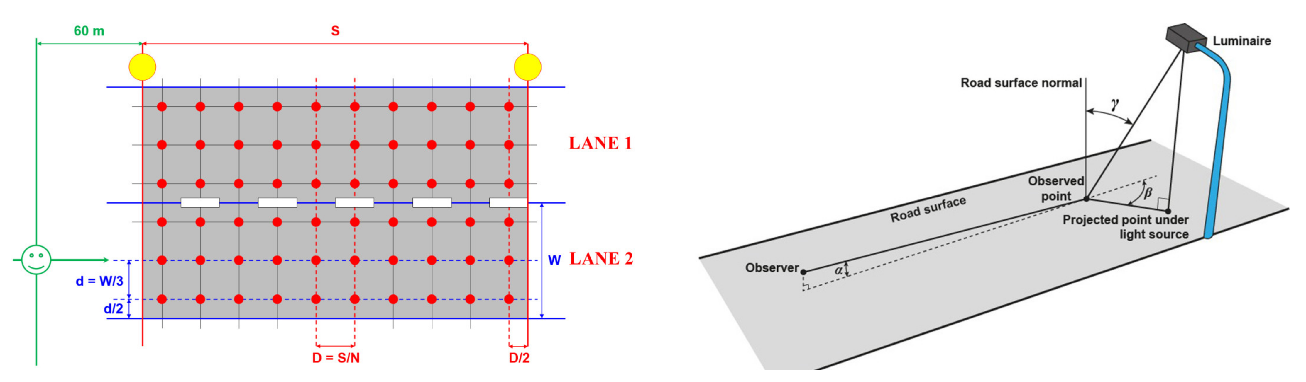
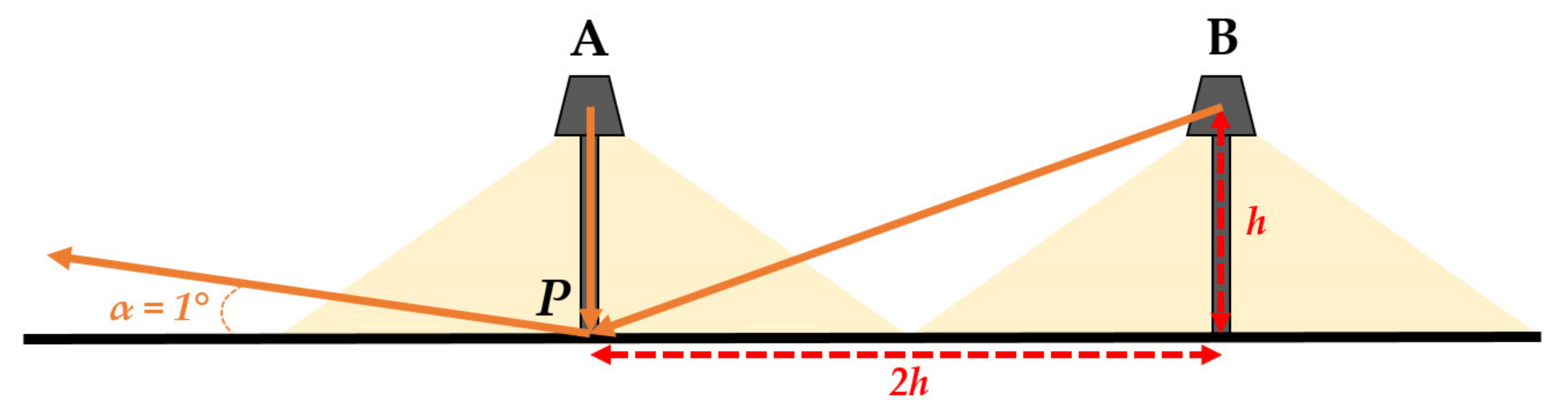

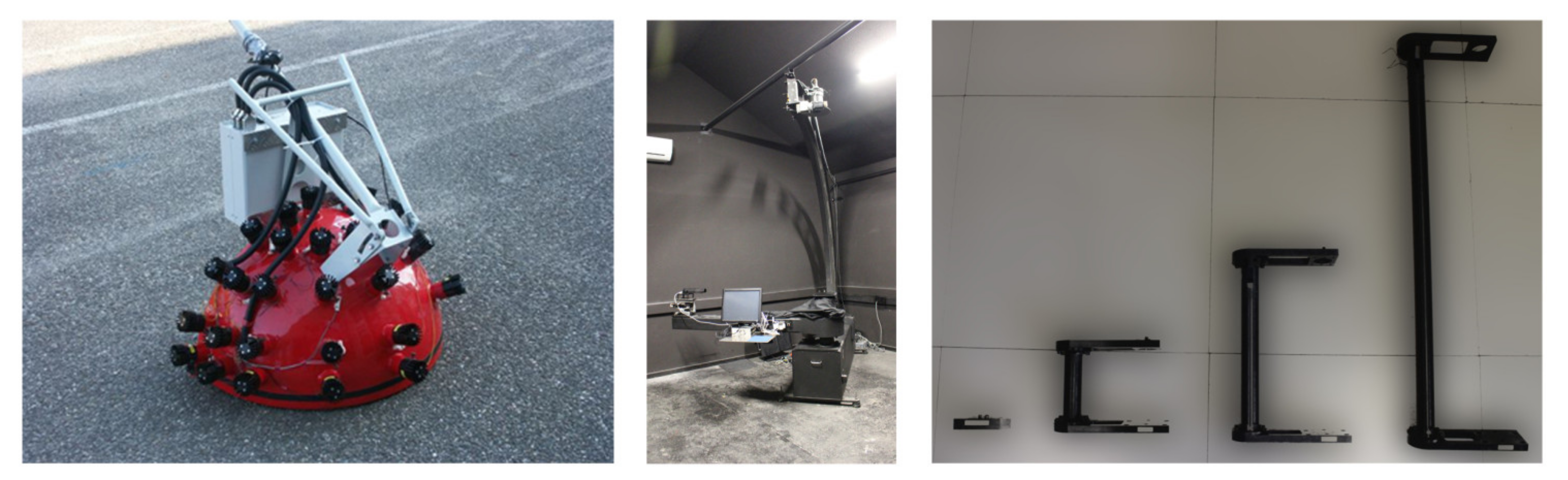
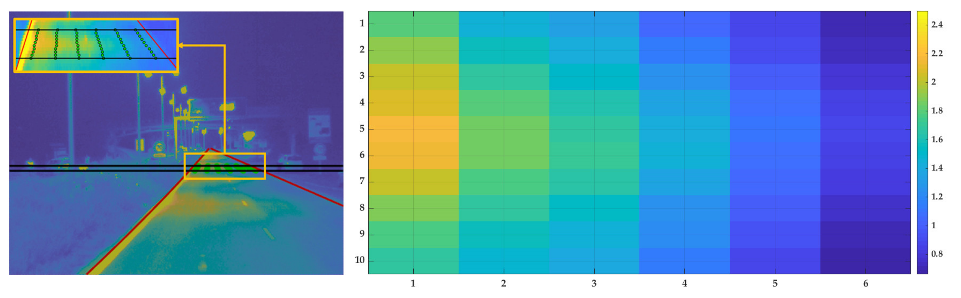
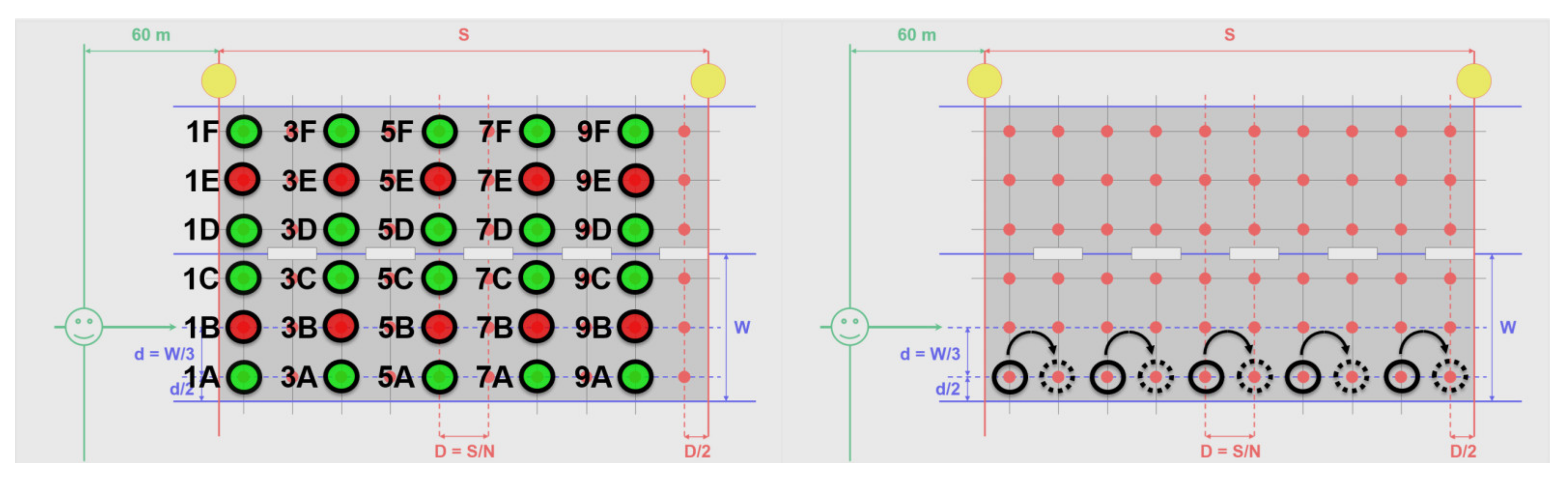
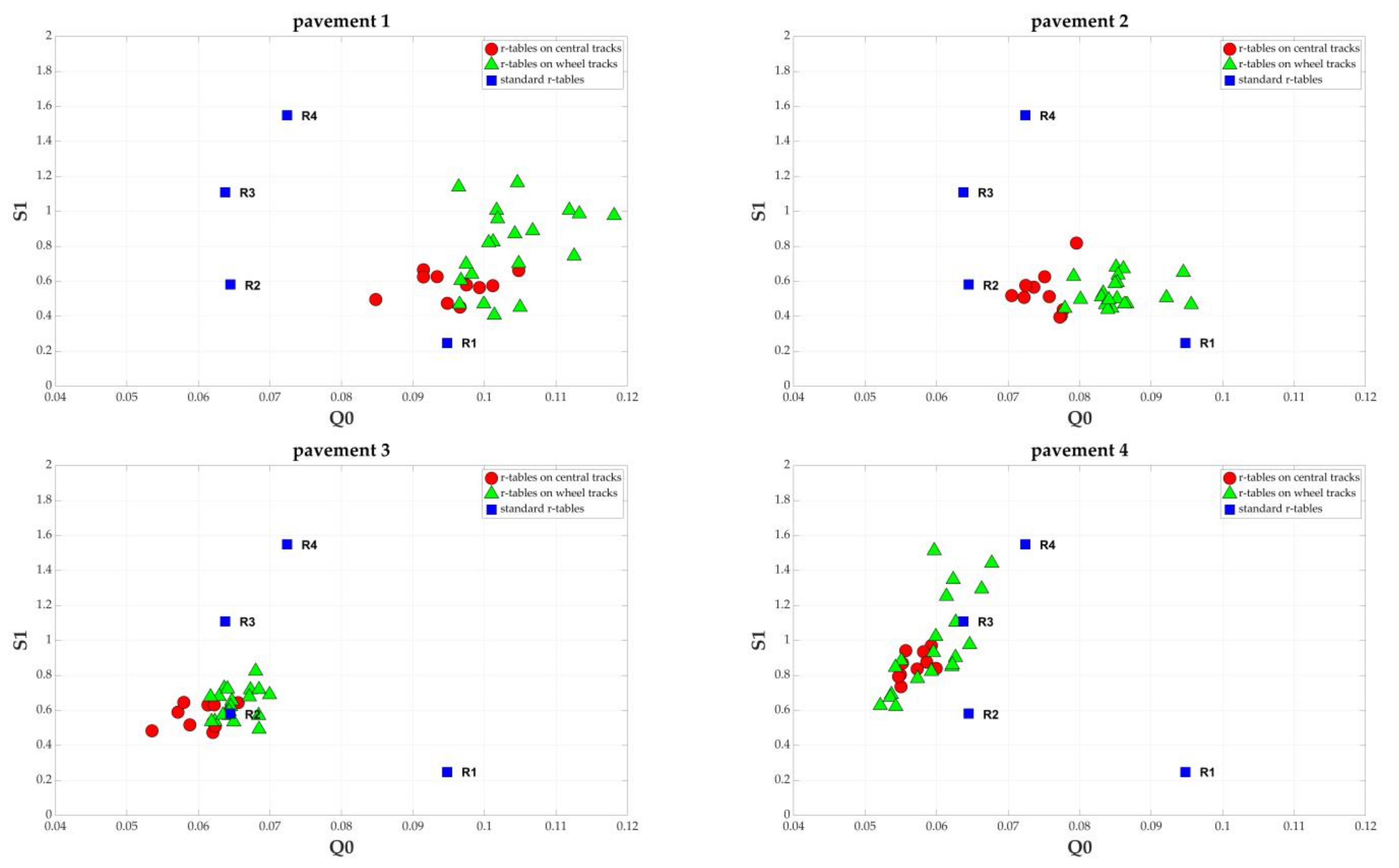

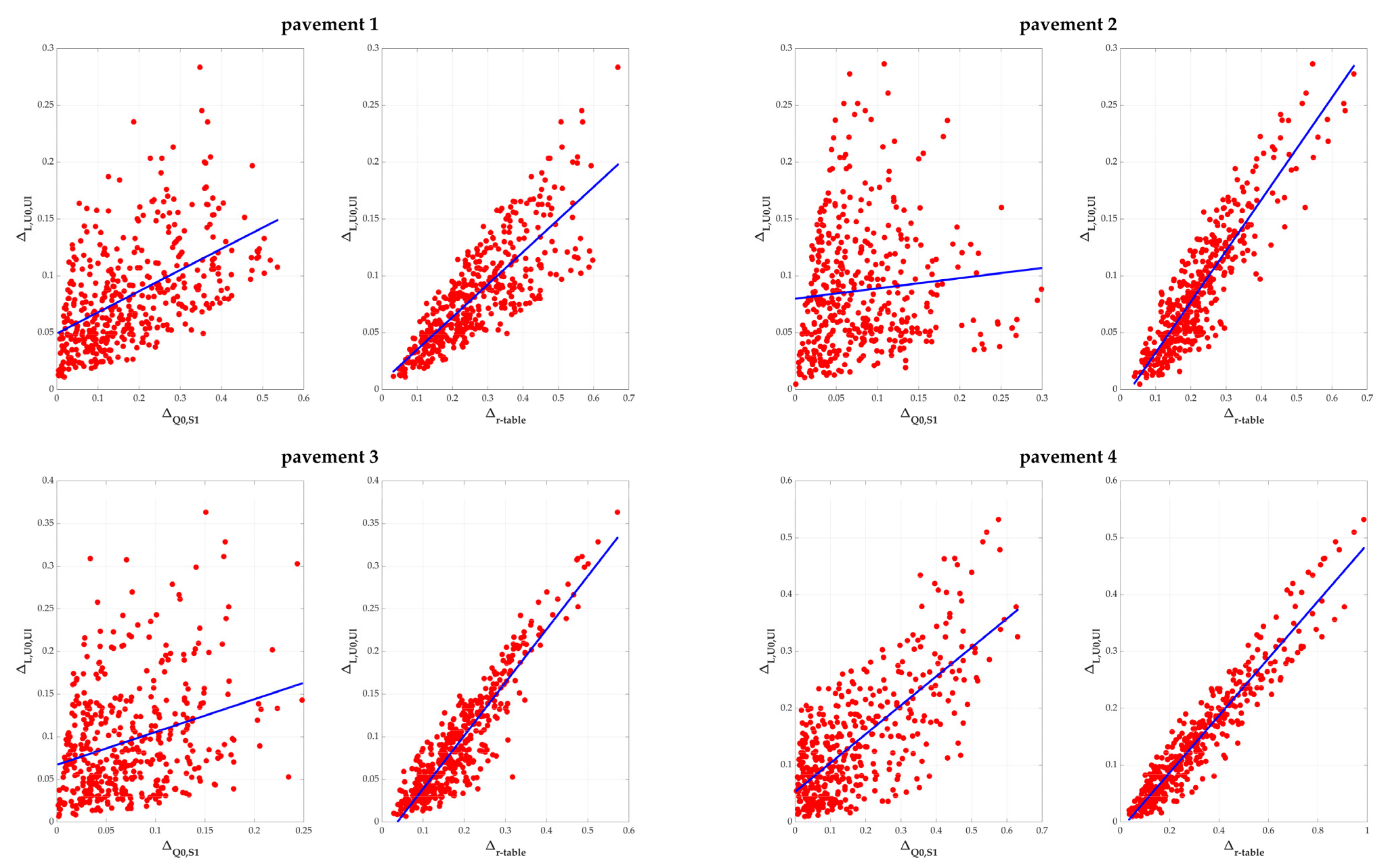
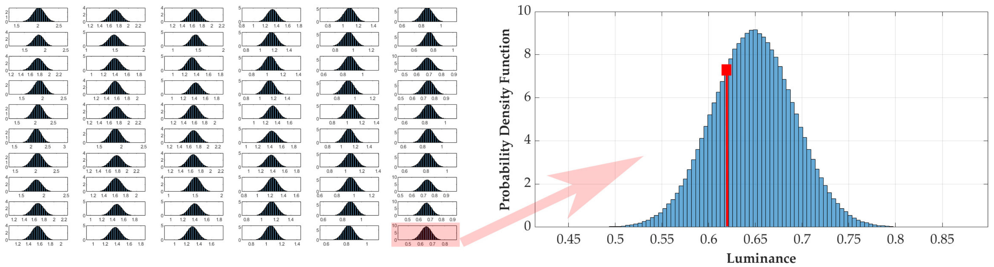

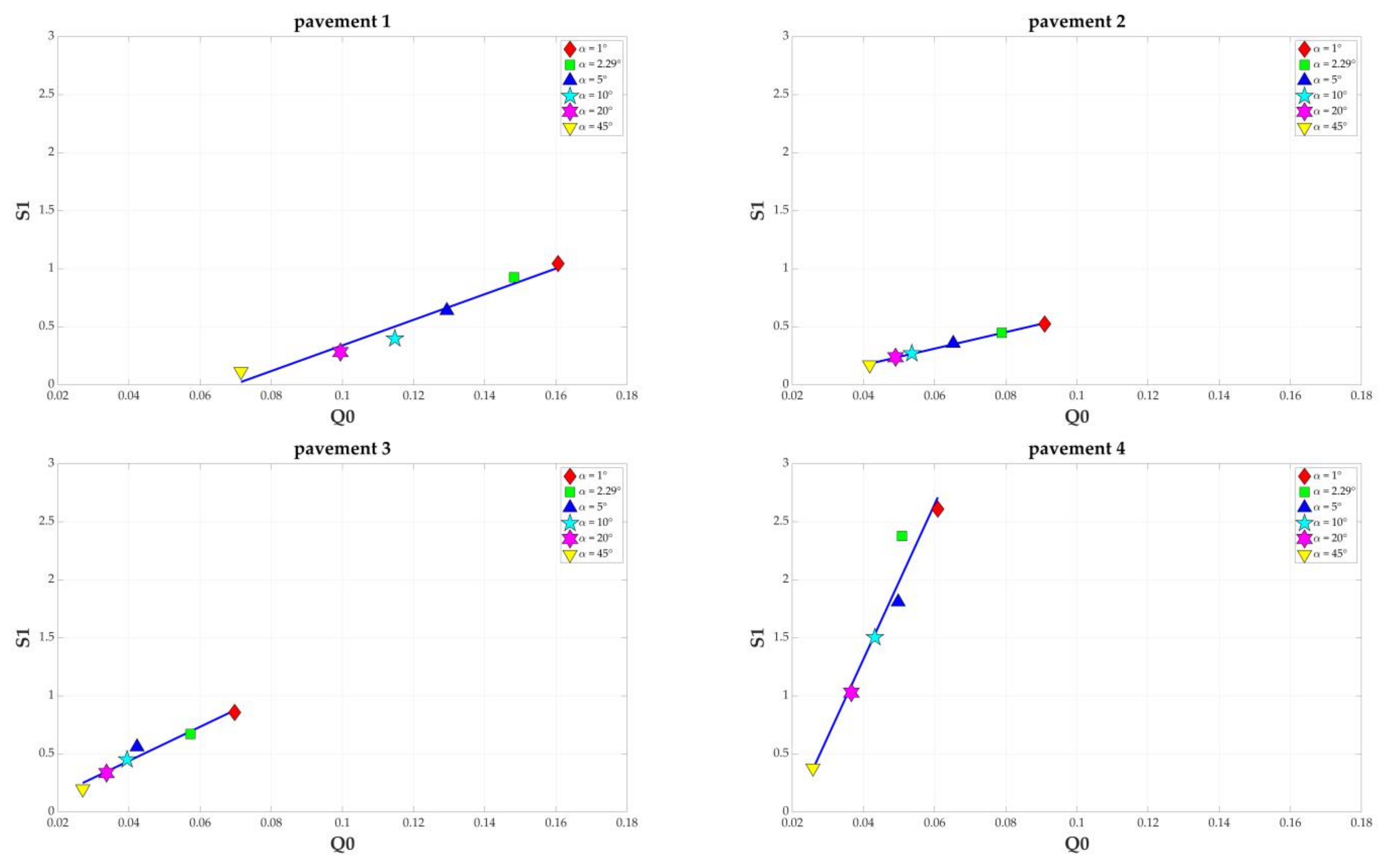
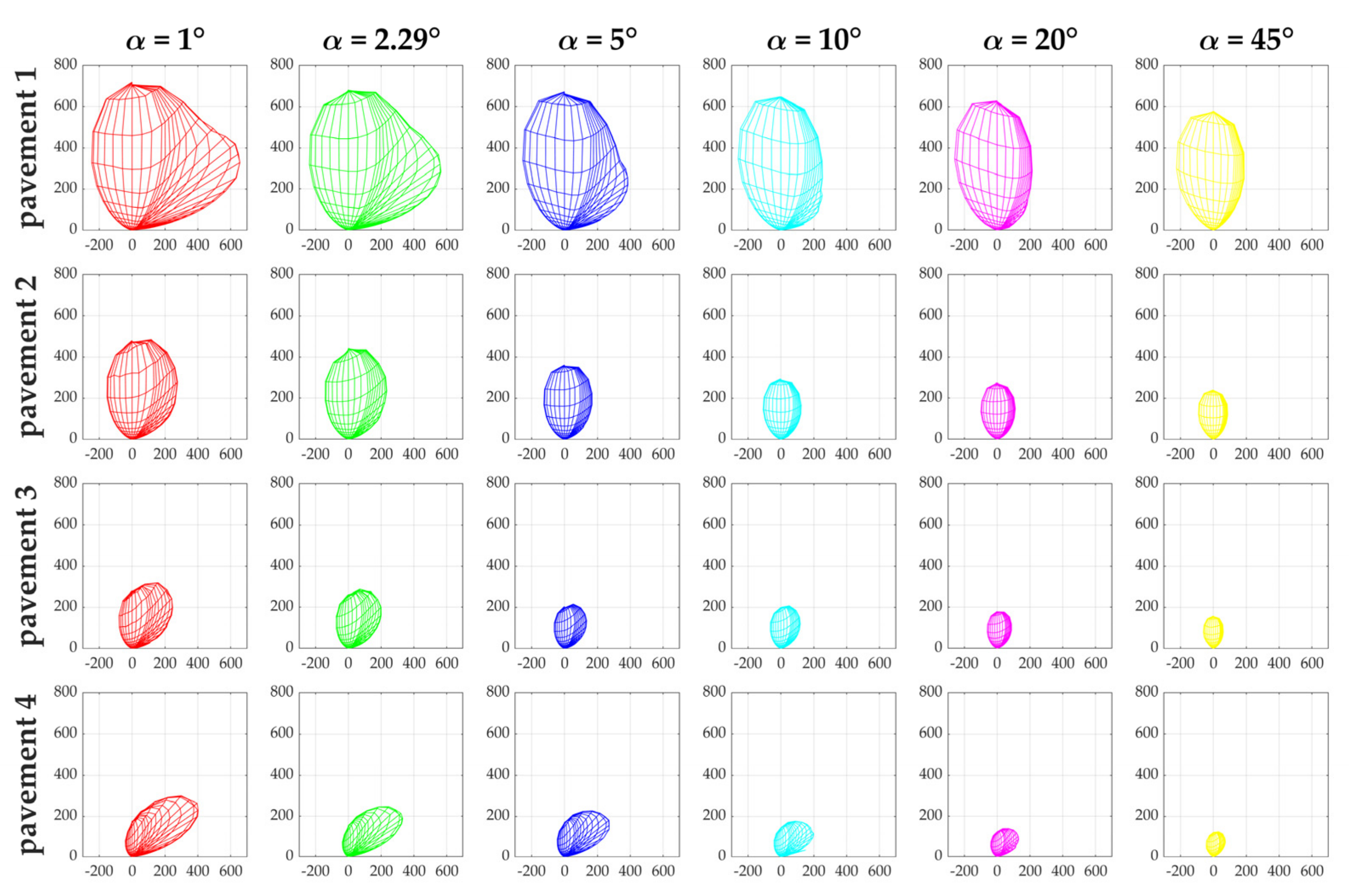
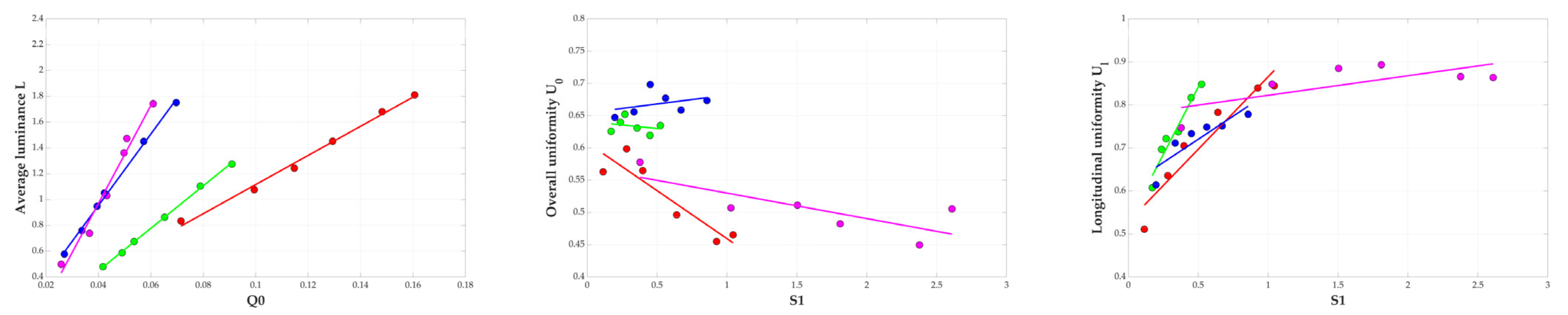
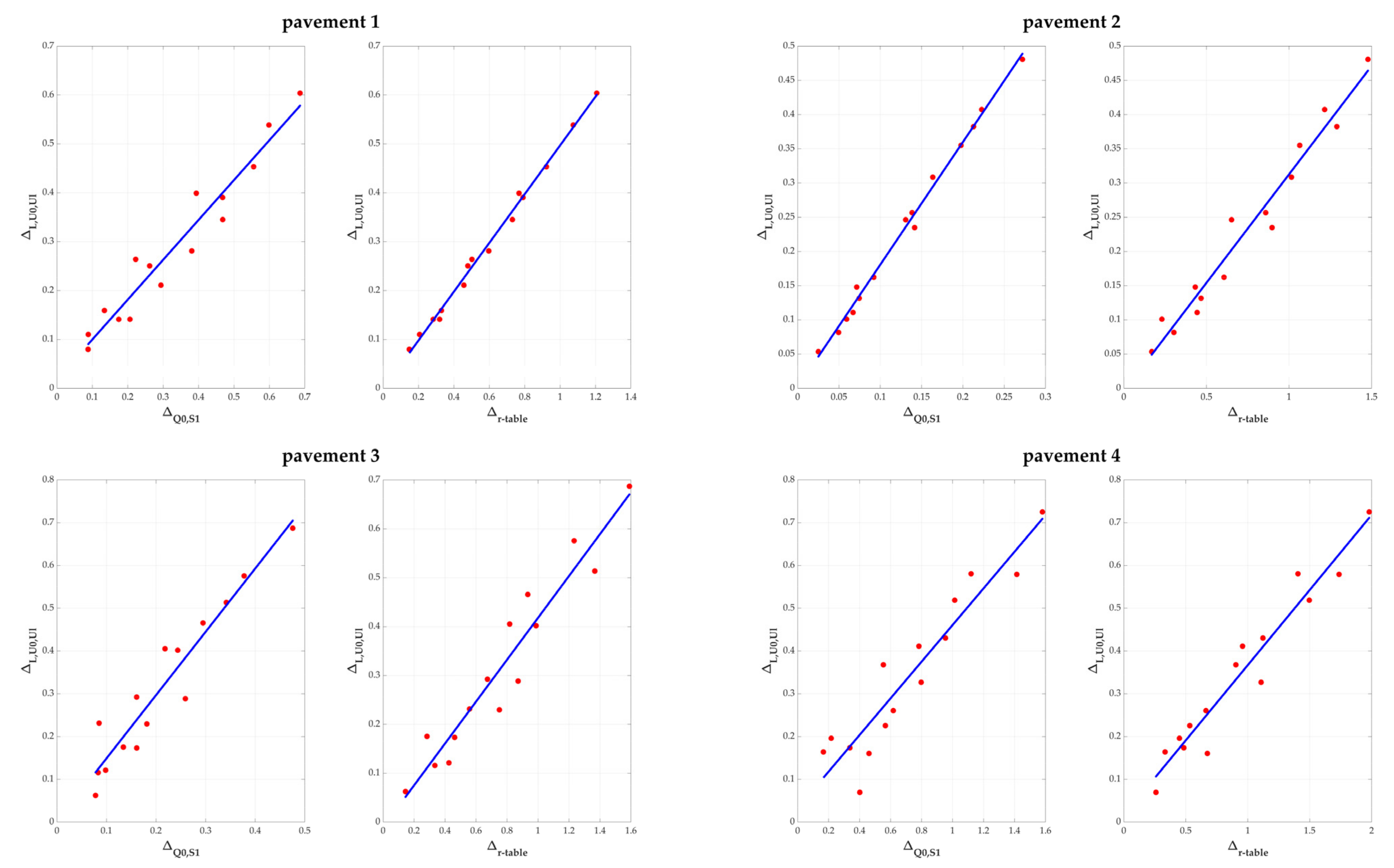
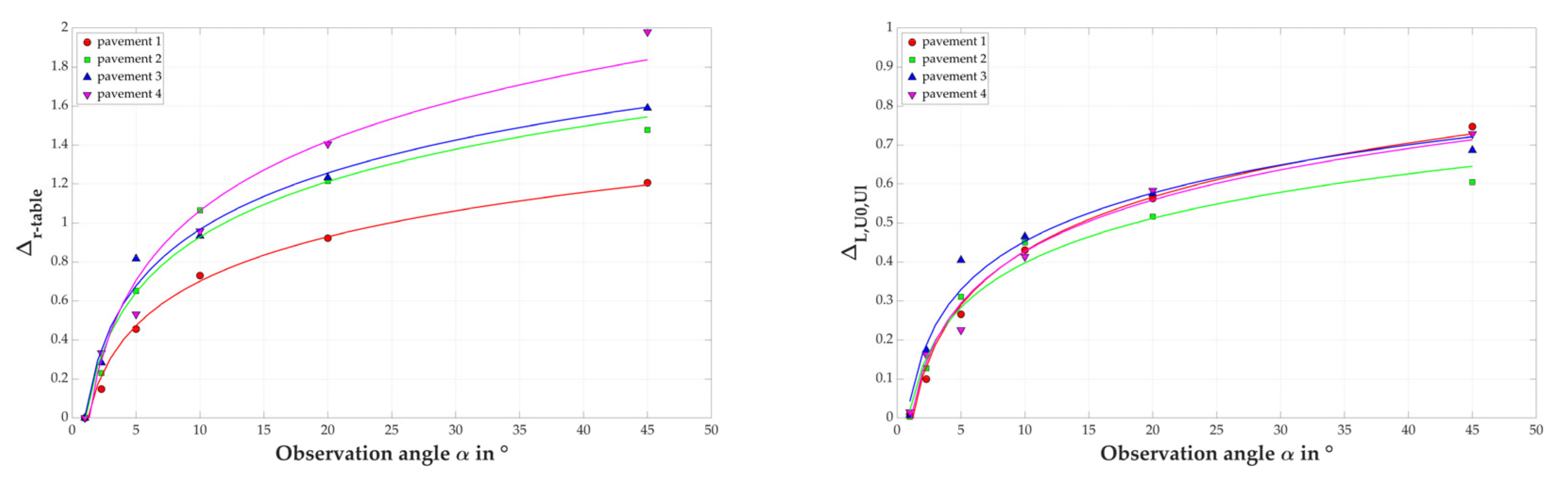
Publisher’s Note: MDPI stays neutral with regard to jurisdictional claims in published maps and institutional affiliations. |
© 2021 by the authors. Licensee MDPI, Basel, Switzerland. This article is an open access article distributed under the terms and conditions of the Creative Commons Attribution (CC BY) license (https://creativecommons.org/licenses/by/4.0/).