Article

Soil and Climate Characterization to Define Environments for Summer Crops in Senegal

by
Carlos Manuel Hernández
1,*,
Aliou Faye
2,
Mamadou Ousseynou Ly
3,
Zachary P. Stewart
4,
P. V. Vara Prasad
1,5,
Leonardo Mendes Bastos
1,
Luciana Nieto
1,
Ana J. P. Carcedo
1 and
Ignacio Antonio Ciampitti
1,*
1
Department of Agronomy, Kansas State University, Manhattan, KS 66506, USA
2
ISRA Regional Centre of Excellence on Dry Cereals and Associated Crops, Thies 3320, Senegal
3
National Centre for Livestock Research (CRZ), Kolda 2312, Senegal
4
USAID, Bureau for Resilience and Food Security, Washington, DC 20523, USA
5
Sustainable Intensification Innovation Lab, Kansas State University, Manhattan, KS 66506, USA
*
Authors to whom correspondence should be addressed.
Sustainability 2021, 13(21), 11739; https://doi.org/10.3390/su132111739
Submission received: 16 September 2021 / Revised: 13 October 2021 / Accepted: 18 October 2021 / Published: 24 October 2021

Abstract

:
Investigating soil and climate variability is critical to defining environments for field crops, understanding yield-limiting factors, and contributing to the sustainability and resilience of agro-ecosystems. Following this rationale, the aim of this study was to develop a soil–climate characterization to describe environmental constraints in the Senegal summer-crops region. For the soil database, 825 soil samples were collected characterizing pH, electrical conductivity (EC), phosphorus (P), potassium (K), cation exchange capacity (CEC), and total carbon (C) and nitrogen (N). For the climate, monthly temperature, precipitation, and evapotranspiration layers were retrieved from WorldClim 2.1, CHIRPS and TERRACLIMATE. The same analysis was applied individually to both databases. Briefly, a principal component analysis (PCA) was executed to summarize the spatial variability. The outcomes from the PCA were subjected to a spatial fuzzy c-means algorithm, delineating five soil and three climate homogeneous areas, accounting for 73% of the soil and 88% of the climate variation. To our knowledge, no previous studies were done with large soil databases since availability field data is often limited. The use of soil and climate data allowed the characterization of different areas and their main drivers. The use of this classification will assist in developing strategic planning for future land use and capability classifications.

Graphical Abstract

1. Introduction

Senegal current population of 17.2 million [1] is projected to double by 2050, requiring greater food production to meet the increasing demand [2]. In this context, improving our understanding of the impact of climate drivers on the crop production and their effects on food security [3,4,5], especially in the developing countries in the West Africa region [2] is a critical need. The effect of climate shocks and their impact on the community is one of the most relevant questions in agriculture for the next decades.
Quantifying the impact of climate shocks is even more critical in countries such as Senegal that rely heavily on rainfed agriculture and livestock systems [6]. Food security has been a top priority over the last several decades, even more due to the reported variability in precipitation distribution and its seasonal patterns [7]. Climate drivers such as erratic precipitation and more extreme events represent a serious threat to food security [8]. This is especially relevant to smallholder farmers based on their specific environments due to a lack of access to timely information and limited resources to adapt to climate variability. This clearly demonstrates that spatial variability plays a critical role in the vulnerability to food security in the country and region.
Studying the variability of the environment, focusing on soil and climate, is a critical step forward to understanding the potential effects of these stressors on crop production and food security. From a soil perspective, little is known about the long-term impact of soil changes on crops [9]. Teluguntla et al. [10] showed a clear linkage between soil degradation and its impact on crop production in major crop-producing regions around the globe. Further, efforts to reduce soil degradation represent a challenge to ensure soil and food security [9]. Koch et al. [11] defined the concept of “soil security” as the maintenance and improvement of soils worldwide to achieve continued availability of the soil resources so that they can continue to provide food and other environmental services. Its relation to food security is critical to establishing a more sustainable pathway maintaining future gains in crop productivity while reducing the impact of this process on the continuous degradation of soils (i.e., loss of soil structure, nutrients, and erosion; [12]). For resource-constrained farmers, the improvement of soil health is critical to providing economic return to fertilizer inputs [13]. A recent large survey highlighted key biophysical and socio-economic barriers and potential opportunities and solutions to address soil fertility issues in Africa [14]. They clearly indicated the soil fertility should be viewed as a means not just to improve productivity but also to provide nutritious food and improve the livelihoods and wellbeing of people. In the last decade, the AfSIS (Africa Soil Information Service) project aimed to compile datasets to improve soil characterization in Africa [15,16]. By collecting new topsoil data, this project was able to finalize a soil mapping of relevant soil properties (e.g., organic carbon, pH, total nitrogen, exchangeable bases) of Africa at 250 m resolution [17]. This is a clear step forward to improve soil characterization and understanding the impact of crop production on short- and long-term soil security. However, the current resolution is still large to represent conditions of smallholder farmers and suffers from greater uncertainty in zones with low validation data density. Therefore, soil information at finer scales to better address localized food and soil security issues, especially in relation to climate shocks, is lacking [3,18,19]. Such soil fertility mapping and characterizing could be a good step for better understanding soil fertility challenges and opportunities and consequent fertilizer application accuracy since Senegal has, for cereals and legumes, a flat fertilizer recommendation applied across the country regardless of climate and soil variability.
The effect of climate variation (mainly described as changes in temperatures and precipitation patterns) and its impact on food security and smallholder farmer income is a research priority [3,20]. Higher temperature (projected to rise faster in West Africa; [21]) and water-deficit threatens global crop productivity and food security [22]. Most of the food grain crops are highly sensitive to short periods of high temperature stress events during flowering and early grain periods leading to lower crop yields [20]. Thus, a regional climate classification based on both spatial and temporal climate variability is important to understand the impact of climate shocks on crop yields [23]. An initial and needed step is to obtain a more automated process to classify the most relevant agricultural regions and therefore understand the main factors driving changes and limitations related to crop suitability. Moreover, sensitivity to climate shocks is severely impacted by soil security, with land degradation more rapidly exposing the vulnerability of crop production and its spatio-temporal variation [24]. The lack of a soil–climate classification implies that potentially much of the crop selection and practices implemented in one region are overlooking the heterogeneity of these relevant classification factors. In the face of increasing extreme climate conditions and soil degradation, improving both spatial and temporal classifications of soil and climate variabilities is a critical step for land use planning [25]. In addition, this soil and climate classification is relevant to delineate homogeneous zones with similar environmental effects on the crops, assisting in developing strategic planning and improving future land capability classifications [26].
This study focuses on Senegal, as a case study, to develop a useful environmental classification based on soil and climate datasets, focused on the main region for the summer field crops. The overall goal was to describe the main environmental constraints to crop productivity in this region, counting with a large soil sampling dataset (825 soil samples) to achieve it. The specific goals of this project were to (i) map the soil variation and identify the main factors driving changes in the classification process and following a similar approach and (ii) describe the climate variation and identify the most relevant climate driving factors defining homogeneous zones for adaptation of field crops in the region.

2. Materials and Methods
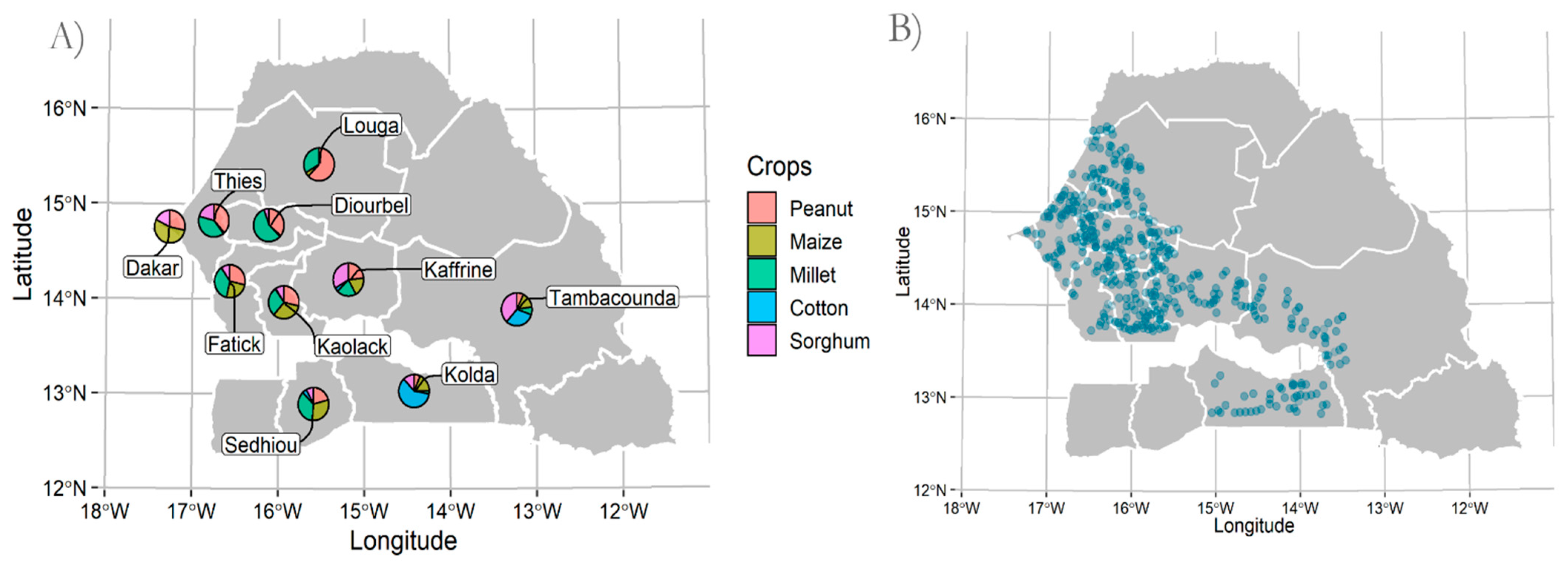
2.1. Study Area

The study was conducted in the Senegalese Sudano-Sahelian region between latitudes 16.13° N and 12.62° N and the longitudes −17.55° W and −12.47° W. This zone has an area of 75,283 km2 and includes 10 administrative regions (Saint Louis, Louga, Thies, Dakar, Diourbel, Fatick, Kaolack, Kaffrine, Tambacounda, and Kolda). The climate of the country is characterized as dry tropical in the south and semi-arid with sparse vegetation towards the north [27,28]. Precipitation has a high spatio-temporal variability [29], spatially characterized by a north–south gradient from 300 to 1300 mm, respectively [30], and temporally concentrated during the rainy season (from June to October) with greatest volumes in August. The distribution of the precipitations defines the potential for the crop-growing season during the summer period. The historical average annual temperature is between 24.5 and 29 °C [31]. The dominant soil order in the region corresponds to Lixisols [32], described as sandy and ferruginous [33]. The landscape is plain within a low altitude topography (overall not greater than 130 m.a.s.l), except in the southeast region where the topography rises up to 581 m.a.s.l. [34].
The land use is dominated largely by livestock on rangeland and extensive agriculture [27]. The foremost management practices applied to the livestock production systems are pastoral, agro-pastoral, and off-land systems [35]. Coupled with these less-intensive input production systems, summer crops prevail in the extensive agriculture during the rainy season and forage during the dry season. In the studied region, the most relevant crops are pearl millet (Pennisetum glaucum L.), rice (Oryza sativa L.), sorghum (Sorghum bicolor L.), groundnut (Arachis hypogaea L.), and cotton (Gossypium hirsutum L.) [27,36], with millet as the most frequently grown (Figure 1A) (Table 1).

2.2. Data Sources and Processing
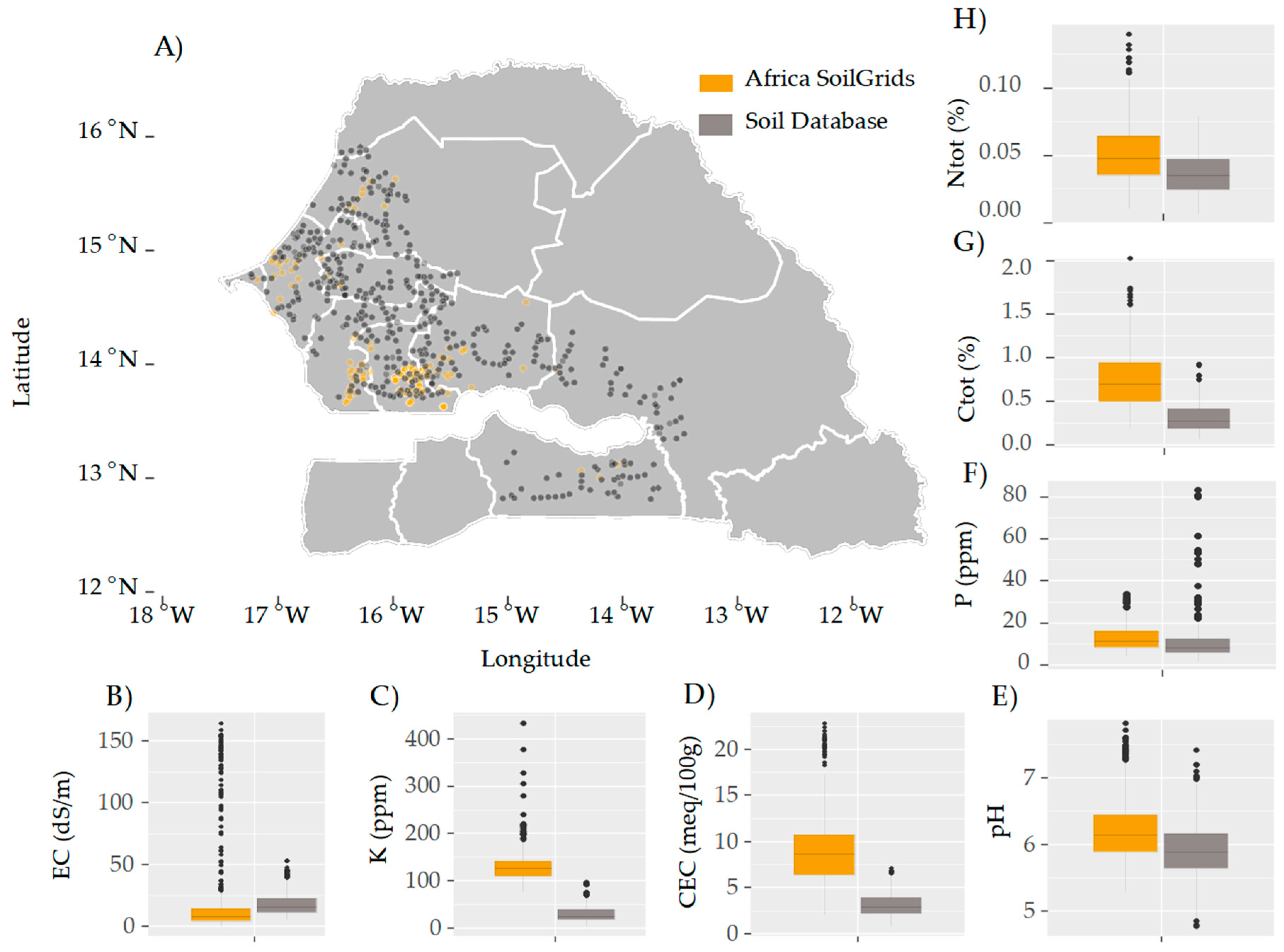
2.2.1. Soil Data

Soil data were obtained from soil samples collected across the study area, from the upper 10 cm, during the 2019 crop season (825 soil samples total, Figure 1B). Soil samples were analyzed for pH-water (potentiometric, CN-TM-S02), electrical conductivity (EC, potentiometric, CN-TM-S01), phosphorus (P), potassium (K), and cation exchange capacity (CEC)—all these elements via Mehlich-3 using ICP-OES (CN-TM-S07), total carbon (Ctot), and total nitrogen (Ntot) (CN analyzer, combustion, CN-TM-S54). These variables have been defined as the most relevant for characterizing the chemical soil properties and explaining variations in millet yields [38], which is one of the most relevant crops in the region [37]. The spatial distribution of each soil variable over study area is presented in Figure 2.
The collected soils data were compared with Africa SoilGrids [17] to better understand the importance of the current soil dataset and overall variations, through (i) the ratio between the density of collected samples within the region, and (ii) the overall range of variation of each soil parameters between datasets using a qualitative approach. The depths selected from the Africa SoilGrids layers were pH-EC-CEC-Ctot: 0–5 cm, K-P: 0–30, and Ntot: 0–20 cm. All soil data layers were obtained from: Africa SoilGrids, Afsis250m, and Afsis250m nutrient [16,17].
Data cleaning is a key step for spatial analysis, with geospatial datasets often containing anomalies that are not representative of the global dataset [40]. Thus, we detected outliers (observations that are outside a statistical distribution or that do not follow a general pattern in a data set [41]) and spatial outliers (observations within the general range of variation, which differ significantly from data that is close to their spatial location). Firstly, we detected outliers using the interquartile interval method [42]. Briefly, this method uses the 25th quartile (q1) and the 75th quartile (q3) (defining the interquartile-range; IQR) as upper and lower limits to define values outside of this range as outliers [43,44].
I Q R = q 3 q 1
U p p e r   t h r e s h o l d = q 3 + 1.5 × I Q R
L o w e r   t h r e s h o l d = q 1 1.5 × I Q R  
Secondly, we identified spatial outliers via utilization of Moran’s local index [45,46,47]. The outliers represented 3.6% and the spatial outliers 7.3% of all observations in the soil dataset. Lastly, several methods have been developed for dealing with outliers. An approach widely used for masking spatial data is the use of disk smoothing through a moving median window [48]. In our study, outliers were not removed but spatial smoothing was implemented, determining the locally weighted median using a neighbor set and masking the data classified as outlier or spatial outlier [49]. The neighbor set can be based in different ways. For this work, we used k-nearest neighbors, taking into account that k = 6.

2.2.2. Climate Data

Three main climate descriptors were retrieved: average air temperature (WorldClim 1.2; [50]), precipitation (CHIRPS; [51]), and potential evapotranspiration (TERRACLIMATE; [52]). These variables represent some of the most important variables for characterizing the climate effect on crops [4,53,54,55,56]. Main details on data sources can be accessed in Table 2.
Climate data were downloaded for the period from 2010 to 2020 (10 years) and further filtered to include only the growing season relevant to summer crops (from May to November). The CHIRPS (Climate Hazards Group InfraRed Precipitation with Station Data) and TERRACLIMATE data sources were accessed via Google Earth Engine (GEE) platform, application programming interface (API) with Python using the geemap [57] and the GEE library [58]. Unlike the rest of the data sources, CHIRPS provides the precipitation layers in daily steps. In order to match the other variables (monthly average temperature from WorldClim 2.1, and monthly average evapotranspiration from TERRACLIMATE), data were aggregated through the sum of the precipitation within each month. Later, the monthly temperature, precipitation, and evapotranspiration were average across years (n = 10) to build one layer for each variable for each month. Moreover, the pixels were average and rescaled to 3500 m resolution to match the resolution with the soil dataset. Lastly, all the weather variables layers were stacked and cropped using the study area as a mask layer. This procedure was performed using the “raster” package [59], in R software [60].

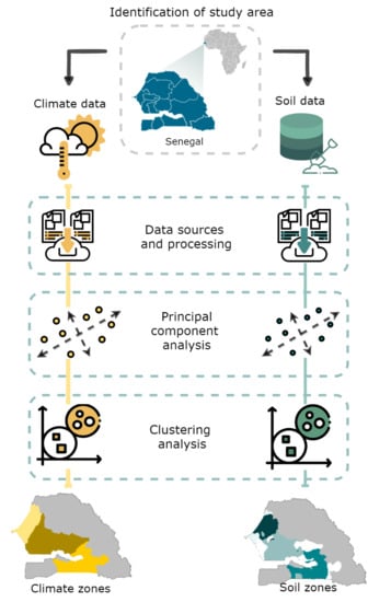
2.3. Protocol Sequence

The following protocol sequence was executed in two steps: firstly, using the soil dataset, and secondly, using the climate datasets. This approach recognizes the value of the classification of soil and climate as separate products, underlining the relevance of the observed soil data availability of this study.

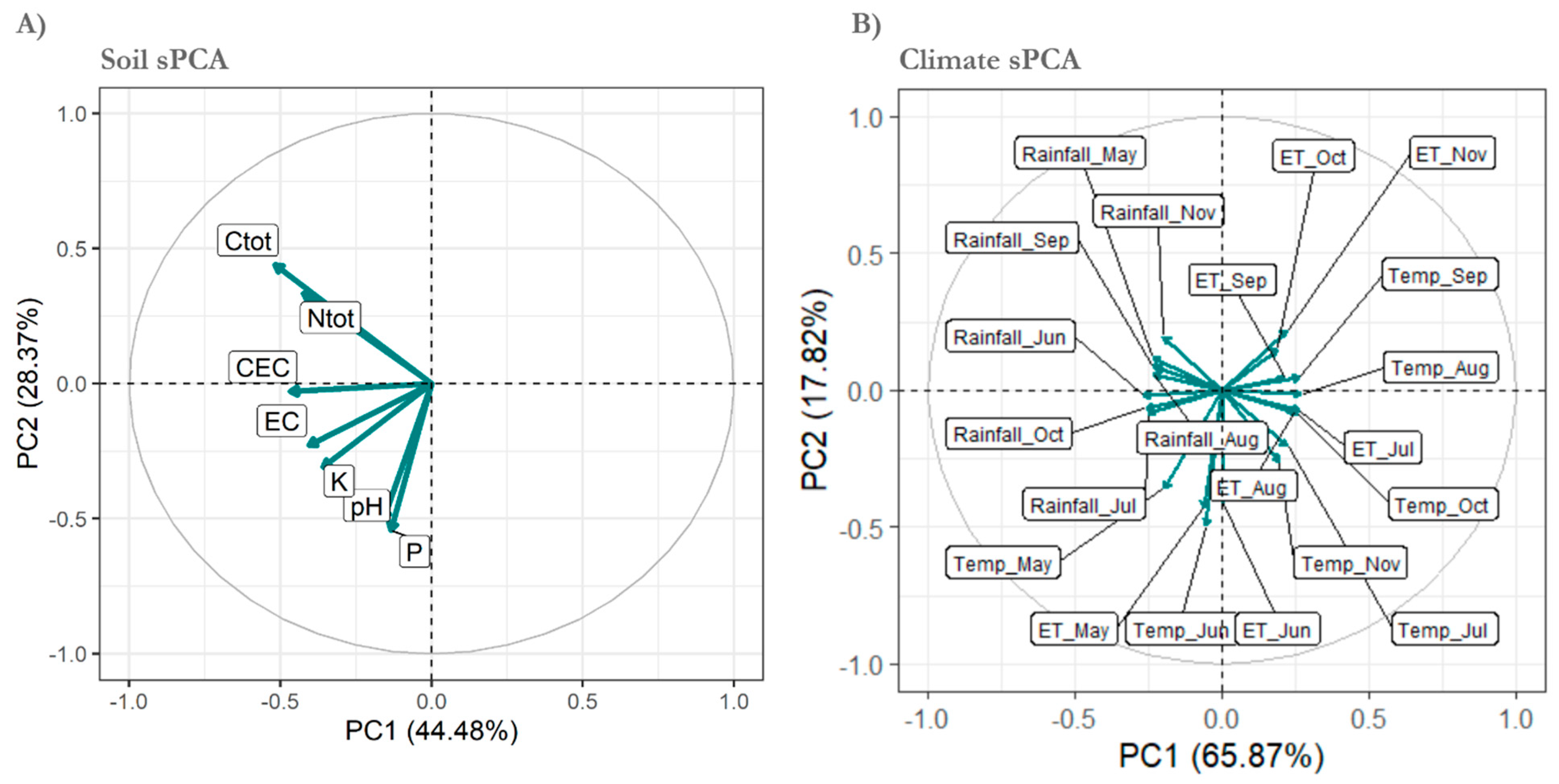
2.3.1. Principal Component Analysis

Feature reduction techniques are used to reduce the dimension in the datasets. Several methods have been developed for dealing with data dimensionality. Among them, principal component analysis (PCA), a multivariate technique, has been widely used in the sciences, engineering, and commercial applications to reduce the number of variables [61]. This technique allows identifying the dimensionality and the latent structure of data [62]. This method captures different types of variability in the data, summarizing them as components made up by linear combinations of the original variables. However, spatial datasets have intrinsic characteristics, such as spatial autocorrelation and spatial heterogeneity, that need to be considered. Recently, different approaches have been used to account for the spatial component in the data [63]. In this study, we used spatial PCA (MULTISPATI-PCA, [64]) to perform layer integration and feature reduction. Unlike conventional PCA, the MULTISPATI-PCA is a type of PCA with spatial restrictions that are introduced through a spatial weighting matrix to calculate correlations among the original data. These spatial restrictions are included via the definition of spatial autocorrelations using Moran’s index and a network of neighboring observations of each data point [65]. The set neighbor was determined based on parameters obtained through semivariograms fitted to each dataset (with a relative structure variability above 40%), establishing 20,000 m as the maximum distance for the soil dataset and 50,000 m for the climate dataset. This method has been executed using interactive variogram estimation with the eyefit function of geoR package. This approach has been broadly implemented in different environments [66,67,68,69].
Lastly, to generate a continuous layer of the study area, the first and second spatial principal components (sPC) were interpolated. A kriging methodology was used to interpolate the sPCA of soil variables. In contrast, for the climate, sPCA used a regular grid to extract the values of centroids of the pixels of climate raster layers creating a climate database with the monthly data for cumulative precipitation, average temperature, and cumulative evapotranspiration. The climate variables of this database were used as input data for the climate sPCA.
This procedure encompasses the methodology described by Cordoba [70], using the R packages Ade4 [71], geoR [72], adespatial [64], and Spdep [73], within the statistical software R [60].

2.3.2. Cluster Analysis

In our analysis, for both soil and climate data, the first and second sPCs were selected for further clustering using non-hierarchical spatial fuzzy c-means algorithm [74] with the R package “Geocmeans” [75]. This approach is a logical diffuse algorithm for making cluster analysis, which introduces the spatial component to the fuzzy c-means method. The introduction of the data spatial identity has the aim to produce a spatial smoothing, decreasing the noise in the final outcome [76]. This algorithm classifies based on the degree of similarity of an object to a group by its membership to the group. We used the squared Euclidean distance and a fuzziness coefficient m = 1.3, following the methodology from Odeh [77]. The number of clusters used for zoning was determined considering the minimum number of clusters that explained at least 70% of the inertia (Supplementary Materials, Figure S1A,B).

3. Results

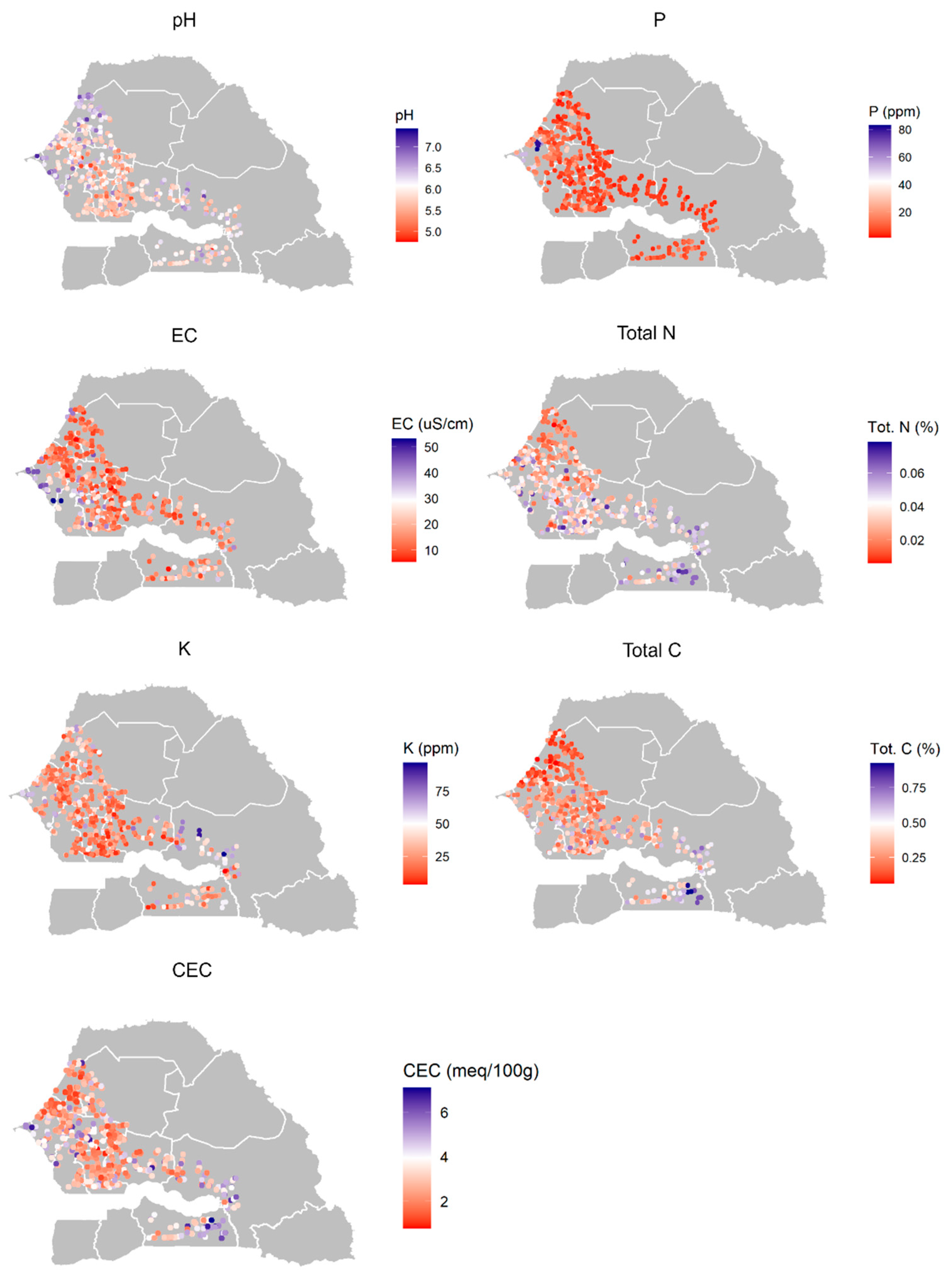
3.1. Environmental Description

Selected soil variables and spatial descriptors are presented in Table 3. Coefficients of variation (CV) ranged between ~7% (pH) and ~94% (P), with a majority of the soil variables presenting high variability (CV > 40%). All variables portrayed a large spatial autocorrelation, with both P and total carbon (Ctot) displaying the largest values for the Moran Index (MI, 0.54 and 0.51, respectively). Positive values of the MI verify the presence of spatial autocorrelation, showing the degree of similarity of a value in a given site with respect to the surrounding data neighborhood.
Focused in the study area, the density of samples per unit area were close to three-fold less for the Africa SoilGrids (n = 282) relative to our collected soil database (n = 825), in addition to presenting a less-uniform geographical representation for Africa SoilGrids with more samples concentrated in the northern region (Figure 3A). Among the explored soil variables, great differences were found for K, CEC, and Ctot. Regarding the variability shown in the boxplots, Ctot and CEC from our database presented greater values ranges than SoilGrids (Figure 3B–H). Overall, Africa SoilGrids overestimate compared to our database, except for EC.
For the climate variables, the monthly cumulative precipitation ranged from 0 to 338 mm, with a mean monthly value of 78 mm (Table 4). Furthermore, this variable showed the greatest CV (24%). In contrast, the average monthly temperature resulted in a CV of 4.3%. This value was the lowest for all climatic variables, with a minimum of 24.7 °C and a maximum of 31.9 °C and showing a mean value of 28.0 °C. Lastly, the water potential atmospheric demand (potential evapotranspiration, ETo) ranged from 115 to 150 mm/month, with a CV of 11%.

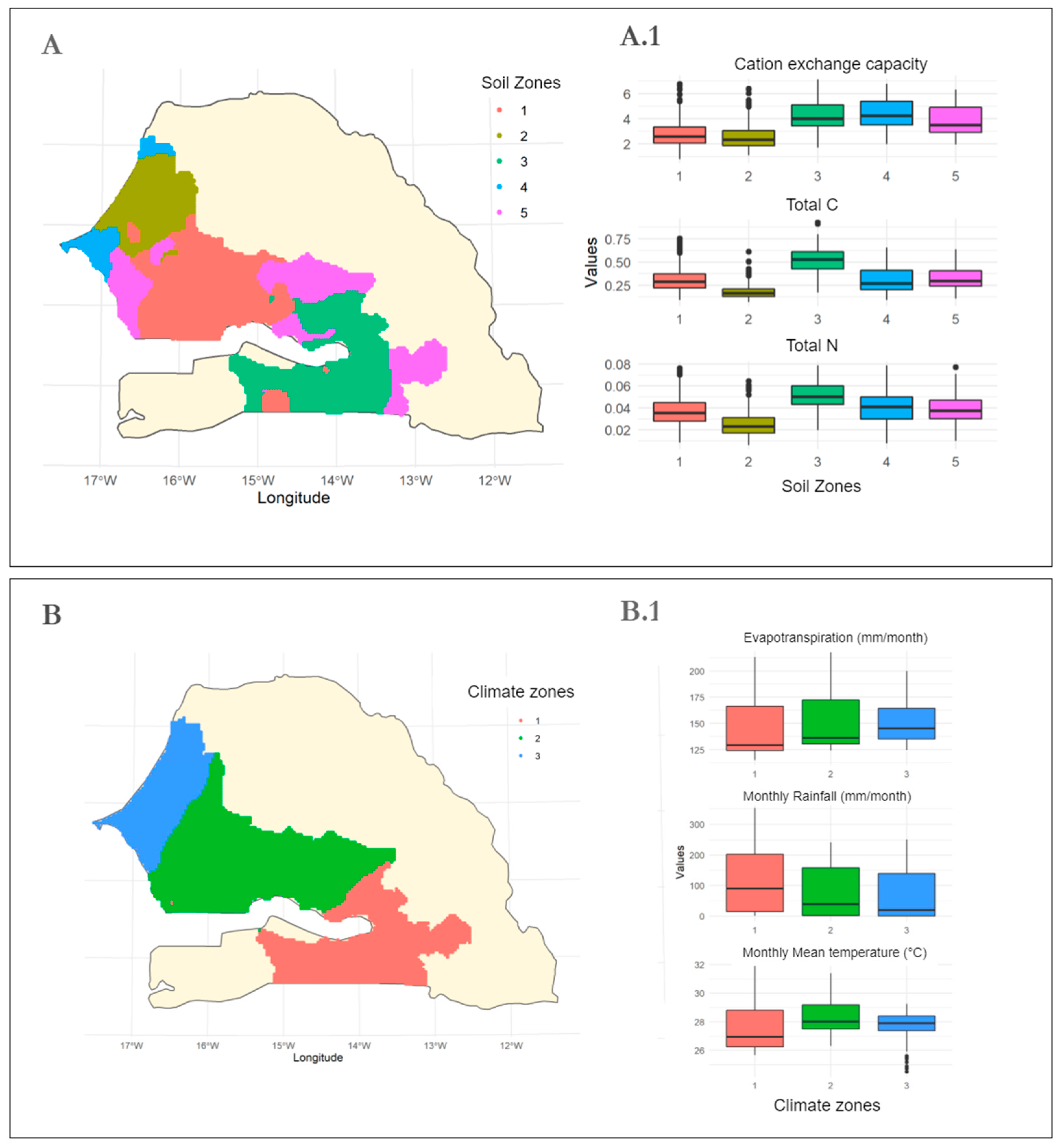
3.2. Soil Classification

As a first step, we executed the variable reduction using the sPCA. The variables that explained the largest proportion of the spatial variability were Ctot, Ntot, CEC, and CE for the sPC1 and pH and P for the sPC2 (Figure 4A). The sPCA applied to the soil data accounted for roughly 73% of the variance between the first and second sPCs (Figure 4A). Figure 4A shows a close association between Ctot and Ntot but not with P and pH factors. Those last soil variables (P and pH) presented a similar direction and association with K. Lastly, CEC, K, and EC presented similar directions, reflecting a high level of association relative to other variables such as Ctot and Ntot or P content for the soils in this region.
The geostatistical analysis applied to sPCs 1 and 2 of soil variables, using semivariogram fitting, showed that the spatial dependence ranged between 3.6 km (sPC1) and 12.7 km (sPC2). The uncorrelated spatial variance, expressed as the nugget variance, were 0.63 and 0.47 for the sPC1 and sPC2, respectively. In contrast, the spatial variance expressed as the sill partial parameter had values between 0.35 (sPC2) and 0.79 (sPC1). Analyzing the values of relative structural variance, sPC1 presented a value of 55% and sPC2 of 42%. These values showed the presence of intermediate spatial variability in both sPCs when compared with reference values [78].
As a result of using the spatial fuzzy c-means clustering analysis with the sPC1 and sPC2 from the soil data, we determined five zones, which accounted for 76% of inertia in the spatial scale (Supplementary Materials, Figure S1A). These five zones represented different geographical areas, with Zones 2 and 4 located to the north of the region, 1 and 5 to the center, and 3 in the south (Figure 5A). Overall, Zone 2 presented the lowest values for CEC, Ctot, Ntot, and EC (as also reflected in Figure 2), while both Zones 3 and 4 had the highest values for these soil features (Figure 5A.1). The main soil factors differing among all zones were related to the variation on the CEC, Ctot, and Ntot.

3.3. Climate Classification

The sPCA applied to the climate data captured nearly 88% of the spatial variance (Figure 4B). The most relevant climate variables described from the analysis were the cumulative precipitation in June, average temperature in August and in September for sPC1, and the average temperature in June and the cumulative potential evapotranspiration of May for sPC2. Three zones were described from the fuzzy c-means clustering analysis, which accounted for 72% of the inertia in the spatial–temporal scale (Supplementary Materials, Figure S1B).
Compared to the soil clustering, the climate zones presented a more defined geographical delimitation, with Zone 3 to the North, Zone 2 in the Center, and Zone 1 to the South. Zone 1 showed greater precipitation (PP), less potential evapotranspiration (ETo), and less average temperature than the rest of zone (116 mm/month, 143 mm/month, and 27.5 °C). The size of the range interquartile in Zone 3 of the analysis of climate data (Figure 5B1) showed lower variation than the other boxes, indicating lower variation within each group. In contrast with this, Zones 1 and 2 exhibited greater variation. The cumulative precipitation displayed an increasing gradient from north to south. The ETo showed the opposite gradient, driven more by temperature.
The spatial variation in water balance (Figure 6A) displayed a gradient that decreased with latitude (greater to the south). Furthermore, August and September were the months with a more positive water balance (Figure 6B).

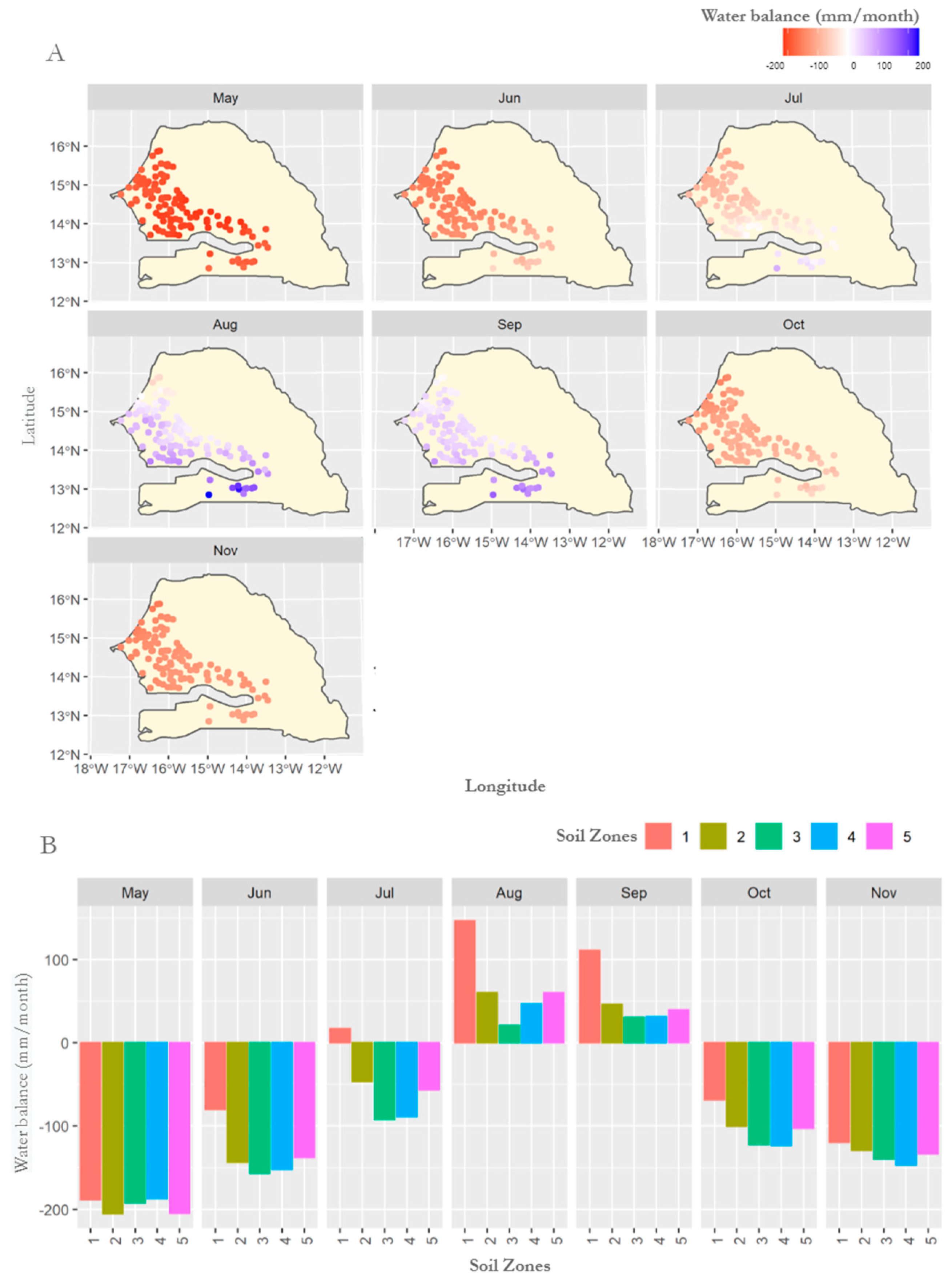
3.4. Relationship between Monthly Climate Patterns among Soil Zones

Contrasting results were found when analyzing the difference between monthly cumulative precipitation and the cumulative ETo for each of the soil zone. Positive water balances were documented for the months of August and September for all soil zones (Figure 6B). The month of May presented the largest negative water balance (<150 mm/month) during the crop growing season. Lastly, the months of October and November were characterized by presenting the lowest water balance, reaching negative values mainly for Zones 3 and 4. Regarding temperature, the greatest differences were found between Zones 1 and 3 (Figure 6B), beginning to decrease early from May to September, and increasing in October and November. In this way, the regions that showed less cumulative precipitation also presented less variation of temperature in the time period selected.

4. Discussion

Our results highlight the potential of the soil and climate classification for generating a baseline dataset to improve strategic planning, land use capability classifications, and improved targeting of technologies. Overall, by using relevant soil features and climate variables, this study was successful in capturing a large proportion of variation and arranging both spatio-temporal variation of these factors in zone. The defined soil and climatic zones could present a relevant impact for future crop mapping and suitability. This could be easily visualized with the current distribution of crops sown for the different zones. For example, there is a greater proportion of area planted with cotton (Figure 1A) in Climatic Zones 2 and 3, (i.e., lower temperatures, and higher rainfall) and the Soil Zones 3 and 5 (i.e., soils with better agronomic characteristics: higher Ctot, Ntot, neutral pH, etc.). Whereas sorghum, millet, and peanut crops were more concentrated in the Soil Zones 1, 2, and 4. (i.e., lower rainfall and higher temperatures). This distribution is in accordance with the crops’ capability to tolerate adverse condition [79]).
The process of clustering and presenting homogeneous regions is critical for improved innovation dissemination and adoption and for scaling technologies shown to be effective under similar soil and climate conditions. One of the most critical aspects of this study is the availability of ground data for the soil classification, representing an advancement in relation to the currently available mapping products; some of these include various databases from different sources, including the HWSD (Harmonized World Soil Database), the Food and Agricultural Organization (FAO) soil map, the International Institute of Applied Systems Analysis (IIASA), the Institute of Soil Sciences—Chinese Academy of Sciences (ISSCAS), the International Soil Reference and Information Center (ISRIC) 2012, and SoilGrids [80,81]. Although many of these soil datasets are relevant to perform more regional-scale investigations, the level of spatial heterogeneity is often overlooked, and it is still a significant issue when developing an environmental classification for smallholder farmers. To the extent of our knowledge, this is one of the first studies providing a ground-data-based environmental classification and developing a more automated method for this process that can be applied to many other countries around the region.
The novelty of this study remains in the use of local data to help improve products of automated spatial prediction frameworks, which can be complementary to this type of analysis. The collected soil dataset could contribute to improving current available machine learning products [17] by integrating a large geographical scale and number of samples for the study area. Although an improvement on the SoilGrids [82] was achieved by including a measure of error (via quantile method) for each estimate, these estimations still do not account for the true uncertainty of the estimate and its process (spatial scale) that can be more formally quantified via the utilization of Bayesian approaches [83]. More recently, Ippolito et al. [26] reported different levels of agreement between SoilGrids and HWSD in the Dosso region of the Niger relative to key soil properties such as pH and texture, among other parameters, and with most of the data collected many years ago, which reduces their relevance for reflecting current soil conditions. The latter scenario of disagreement with local (ground based) soil data and older data sets, without reflecting current management, is a clear constraint when utilizing global datasets to address smallholder solutions. In addition, errors related to more automated approaches and the distribution of observations can limit the scale and applicability of the digital soil mapping [84], increasing the need to obtain more reliable ground data sources at local levels. Likewise for climate data, a similar issue was emphasized by Fall [34]; analyzing long-term mean climate conditions in Senegal (1971–1998) revealed the need for more localized climate data due to the level of scale variation, usually not always captured by gridded global data. We highlight this aspect to be addressed in future studies. This summary clearly pinpoints the need to invest more resources and efforts in developing more relevant terrestrial ground protocols for collecting reliable (and scale for more relevant, 250 m pixel is too large) data for smallholders due to the intrinsic level of complexity, based on the spatial heterogeneity.
This environmental characterization provides a foundational knowledge and dataset for more strategic planning and sustainable agricultural interventions (e.g., reduced tillage, cover crops, crop selection, and use of fertilizers) to deal with such heterogeneity [85,86]. Future tests of the stability of soil and climate zones can improve our understanding of fluctuations linked to climate change. Sustained increases in food supply will need the integration of relevant soil, climate, and crop data with the goal of targeting the right agricultural farming system to the right environment, increasing input use efficiency while reducing the environmental footprint [87]. From the perspective of smallholder farmers, a recent study confirmed that farmers in the region are all well-aware of the impact of changing climate conditions on crop production and the potential adaptations needed to manage the negative effects [88].
Lastly, an increase in the frequency of extreme climate events will require more proactive changes and farmers better equipped with information and knowledge to more rapidly adapt and react to those fluctuations [89]. For example, with the introduction of the short-season dual-purpose pearl millet crop in the region, the adoption of high plant density and balanced fertilization are still obstructed due to lack of economic, institutional (access to credit), and socio-cultural barriers [90,91]. A compromised solution needs to be sought in the near future for securing access to fertilizers via subsidies, providing better credits for other farming inputs, crop insurance, and improving access to data-informed and knowledge-based decision support tools [13,90]. In addition, the complex topics of climate change, climate smart agriculture, sustainable agricultural intensification, and soil fertility management require participatory processes to set research priorities and identify the best solutions [91].
Limitations to the analysis, potentially informing future steps, are related to (1) the lack of temporal variation for soil parameters (e.g., short-term: EC, pH; long-term: P, K, Ctot and Ntot) and vertical soil profiles in order to study the physical limitations (shallow soils), the depth of the soil profile, and the granulometric data of the different soil horizons (relevant for estimation of water holding capacity); (2) the lack of relevant and geo-referenced crop productivity data to validate the soil and climate zone to more formally validate the current classification; (3) the lack of local climate data to benchmark against in order to test the quality of the current regional gridded data sets (WorldClim 2.1, CHIRPS and TERRACLIMATE); (4) the lack of integration of data-informed management practices relevant to the study region; and lastly, (5) the lack of formal integration of remotely sensed products to assist in unbalanced observations for soil and climate data sets and to provide more crop-relevant data.

5. Conclusions

Our main findings were that (i) from the soils perspective, delineating five homogeneous areas with cluster analysis for the soil dataset accounted for roughly 73% of the variation in the spatial scale, with most relevant variables as Ctot, Ntot, CEC, EC, pH, and P; (ii) from a climate perspective, the clustering analysis revealed three climate areas, with the temporal scale portraying August and September as the months with water-positive balance, except for the northern region, and (iii) from the crop suitability standpoint, this study provides insights into the established soil and climate zones and the planted area of the most relevant summer crops in the region. To our knowledge, no previous studies were performed with such a large database of soil samples (825), as field ground-based data are often limited. The use of soil data and climate data allowed the characterization of different areas with contrasting soil and climate patterns in Senegal. These results will be critical for developing strategic planning for future land capability (and land use) classifications and identifying suitability maps for key technologies that can enhance crop productivity, sustainability, and resilience of agro-ecosystems.
Future studies can benefit by including more relevant agronomic (e.g., crop productivity, irrigation practices, and nutrient management), socio-economic (e.g., access to inputs, markets, credit, and land holding) and cultural (e.g., gender, knowledge, and social capital) data from the smallholder farmers in the region to provide a foundational environmental classification relevant to the decision-making process, adoption, and scaling of technologies.

Supplementary Materials

The following are available online at https://www.mdpi.com/article/10.3390/su132111739/s1, Figure S1A,B: Percentage of inertia explained by soil and climate data, Figure S2: Temporal pattern of average temperature and cumulative rainfall among months and soil zones, Table S1: Values of loadings of each variable in the soil data as results of PCA, Table S2: Values of loadings of each variable in the climate data as results of PCA.

Author Contributions

Conceptualization, C.M.H., L.M.B., L.N., A.J.P.C. and I.A.C.; methodology, C.M.H.; software, C.M.H.; validation, C.M.H., A.J.P.C. and I.A.C.; formal analysis, C.M.H.; investigation, C.M.H., L.M.B., L.N., A.J.P.C. and I.A.C.; resources, I.A.C.; data curation, C.M.H.; writing—original draft preparation, C.M.H., L.M.B., L.N., A.J.P.C. and I.A.C.; writing—review and editing, A.F., M.O.L., Z.P.S. and P.V.V.P.; visualization, C.M.H.; supervision, I.A.C.; project administration, I.A.C.; funding acquisition, I.A.C., Z.P.S., A.F. and P.V.V.P. All authors have read and agreed to the published version of the manuscript.

Funding

This study was supported by the Feed the Future Innovation Lab for Collaborative Research on Sustainable Intensification (SIIL) at Kansas State University through funding United States Agency for International Development (USAID) under the Cooperative Agreement (Grant number AID-OAA-L-14-00006). Contribution no. 22-105-J from the Kansas Agricultural Experiment Station.

Institutional Review Board Statement

Not Available.

Informed Consent Statement

Not Available.

Data Availability Statement

Data available upon request from the corresponding author.

Acknowledgments

The team involved in collecting the soils samples from Senegal.

Conflicts of Interest

The authors declare no conflict of interest. The funders had no role in the design of the study; in the collection, analyses, or interpretation of data; in the writing of the manuscript; or in the decision to publish the results.

References

  1. United Nations World Population Dashboard Senegal. Available online: https://www.unfpa.org/data/world-population/SN (accessed on 14 September 2021).
  2. Molina-Flores, B.; Manzano-Baena, P.; Coulibaly, M.D.; Bedane, B. The Role of Livestock in Food Security, Poverty Reduction and Wealth Creation in West Africa; FAO: Rome, Italy, 2020; ISBN 9789251323397. [Google Scholar]
  3. Gregory, P.J.; Ingram, J.S.I.; Brklacich, M. Climate change and food security. Philos. Trans. R. Soc. B Biol. Sci. 2005, 360, 2139–2148. [Google Scholar] [CrossRef] [PubMed]
  4. Lobell, D.B.; Burke, M.B.; Tebaldi, C.; Mastrandrea, M.D.; Falcon, W.P.; Naylor, R.L. Prioritizing climate change adaptation needs for food security in 2030. Science 2008, 319, 607–610. [Google Scholar] [CrossRef] [PubMed]
  5. Burke, M.B.; Miguel, E.; Satyanath, S.; Dykema, J.A.; Lobell, D.B. Warming increases the risk of civil war in Africa. Proc. Natl. Acad. Sci. USA 2009, 106, 20670–20674. [Google Scholar] [CrossRef] [Green Version]
  6. FAO. Global Livestock Production Systems; FAO: Rome, Italy, 2011; ISBN 978-92-5-107033-8. [Google Scholar]
  7. Rasmussen, K.; D’haen, S.; Fensholt, R.; Fog, B.; Horion, S.; Nielsen, J.O.; Rasmussen, L.V.; Reenberg, A. Environmental change in the Sahel: Reconciling contrasting evidence and interpretations. Reg. Environ. Chang. 2016, 16, 673–680. [Google Scholar] [CrossRef]
  8. Wheeler, T.; von Braun, J. Climate change impacts on global food security. Science 2013, 341, 1689–1699. [Google Scholar] [CrossRef]
  9. Pozza, L.E.; Field, D.J. The science of soil security and food security. Soil Secur. 2020, 1, 100002. [Google Scholar] [CrossRef]
  10. Teluguntla, P.; Thenkabail, P.S.; Xiong, J.; Congalton, R.; Tilton, J.; Sankey, T.T.; Massey, R. Global cropland area database (GCAD) derived from remote sensing in support of food security in the twenty-first century: Current achievements and future possibilities. Remote Sens. Handb. 2015, II, 1–45. [Google Scholar]
  11. Koch, A.; Mcbratney, A.; Adams, M.; Field, D.; Hill, R.; Crawford, J.; Minasny, B.; Lal, R.; Abbott, L.; O’Donnell, A.; et al. Soil security: Solving the global soil crisis. Glob. Policy 2013, 4, 434–441. [Google Scholar] [CrossRef] [Green Version]
  12. Lal, R. Soil degradation by erosion. Land Degrad. Dev. 2001, 12, 519–539. [Google Scholar] [CrossRef]
  13. Wortmann, C.S.; Stewart, Z. Nutrient management for sustainable food crop intensification in African tropical savannas. Agron. J. 2021. [Google Scholar] [CrossRef]
  14. Stewart, Z.P.; Pierzynski, G.M.; Middendorf, B.J.; Vara Prasad, P.V. Approaches to improve soil fertility in Sub-Saharan Africa. J. Exp. Bot. 2020, 71, 632–641. [Google Scholar] [CrossRef] [Green Version]
  15. Vagen, T.-G.; Winowiecki, L.A.; Desta, L.; Tondoh, E.J.; Weullow, E.; Shepherd, K.; Sila, A. Mid-Infrared Spectra (MIRS) from ICRAF Soil and Plant Spectroscopy Laboratory: Africa Soil Information Service (AfSIS) Phase I 2009–2013; The World Agroforestry Centre: Nairobi, Kenya, 2020. [Google Scholar]
  16. Leenaars, J.G.B.; Kempen, B.; van Oostrum, A.J.M.; Batjes, N.H. Africa soil profiles database: A compilation of georeferenced and standardised legacy soil profile data for Sub-Saharan Africa. In GlobalSoilMap: Basis of the Global Spatial Soil Information System; CRC Press: Boca Raton, FL, USA, 2014; pp. 51–57. [Google Scholar]
  17. Hengl, T.; Heuvelink, G.B.M.; Kempen, B.; Leenaars, J.G.B.; Walsh, M.G.; Shepherd, K.D.; Sila, A.; MacMillan, R.A.; De Jesus, J.M.; Tamene, L.; et al. Mapping soil properties of Africa at 250 m resolution: Random forests significantly improve current predictions. PLoS ONE 2015, 10, e0125814. [Google Scholar] [CrossRef]
  18. Hertel, T.W. Food security under climate change. Nat. Clim. Chang. 2016, 6, 10–13. [Google Scholar] [CrossRef]
  19. Niles, M.T.; Salerno, J.D. A cross-country analysis of climate shocks and smallholder food insecurity. PLoS ONE 2018, 13, e0192928. [Google Scholar] [CrossRef] [PubMed]
  20. Schmidhuber, J.; Tubiello, F.N. Global food security under climate change. Proc. Natl. Acad. Sci. USA 2007, 104, 19703–19708. [Google Scholar] [CrossRef] [PubMed] [Green Version]
  21. Welborn, L. Africa and climate change projecting vulnerability and adaptive capacity. Inst. Secur. Stud. 2018, 14, 1–24. [Google Scholar]
  22. Prasad, P.V.V.; Bheemanahalli, R.; Jagadish, S.V.K. Field crops and the fear of heat stress-opportunities, challenges and future directions. Field Crop. Res. 2017, 200, 114–121. [Google Scholar] [CrossRef] [Green Version]
  23. Schlenker, W.; Lobell, D.B. Robust negative impacts of climate change on African agriculture. Environ. Res. Lett. 2010, 5, 014010. [Google Scholar] [CrossRef]
  24. Gisladottir, G.; Stocking, M. Land degradation control and its global environmental benefits. Land Degrad. Dev. 2005, 16, 99–112. [Google Scholar] [CrossRef]
  25. Garnett, T.; Appleby, M.C.; Balmford, A.; Bateman, I.J.; Benton, T.G.; Bloomer, P.; Burlingame, B.; Dawkins, M.; Dolan, L.; Fraser, D.; et al. Sustainable intensification in agriculture: Premises and policies. Science 2013, 341, 33–34. [Google Scholar] [CrossRef] [PubMed]
  26. Ippolito, T.A.; Herrick, J.E.; Dossa, E.L.; Garba, M.; Ouattara, M.; Singh, U.; Stewart, Z.P.; Vara Prasad, P.V.; Oumarou, I.A.; Neff, J.C. A comparison of approaches to regional land-use capability analysis for agricultural land-planning. Land 2021, 10, 458. [Google Scholar] [CrossRef]
  27. Manlay, R.J.; Cadet, P.; Thioulouse, J.; Chotte, J.L. Relationships between abiotic and biotic soil properties during fallow periods in the Sudanian zone of Senegal. Appl. Soil Ecol. 2000, 14, 89–101. [Google Scholar] [CrossRef]
  28. Diop, L.; Bodian, A.; Diallo, D. Spatiotemporal trend analysis of the mean annual rainfall in Senegal. Eur. Sci. J. ESJ 2016, 12, 231. [Google Scholar] [CrossRef]
  29. Tucker, C.J.; Vanpraet, C.; Boerwinkel, E.; Gaston, A. Satellite remote sensing of total dry matter production in the Senegalese Sahel. Remote Sens. Environ. 1983, 13, 461–474. [Google Scholar] [CrossRef]
  30. Roudier, P.; Muller, B.; D’Aquino, P.; Roncoli, C.; Soumaré, M.A.; Batté, L.; Sultan, B. The role of climate forecasts in smallholder agriculture: Lessons from participatory research in two communities in Senegal. Clim. Risk Manag. 2014, 2, 42–55. [Google Scholar] [CrossRef]
  31. Beal, T.; Belden, C.; Hijmans, R.; Mandel, A.; Norton, M.; Riggio, J. Country Profiles; Sustainable Intensification Innovation Lab. Available online: https://gfc.ucdavis.edu/profiles/rst/sen.html#land-and-water-resources (accessed on 8 April 2021).
  32. FAO. World Reference Base for Soil Resources; World Soil Resources Reports 106; FAO: Rome, Italy, 2014; ISBN 9789251083697. [Google Scholar]
  33. Baldensperger, J.; Staimesse, J.P.; Tobias, C. Notice Explicative de la Carte Pédologique du Sénégal au 1/200000—Moyenne Casamance; ORSTOM: Marseille, France, 1967. [Google Scholar]
  34. Fall, S.; Niyogi, D.; Semazzi, F.H.M. Analysis of mean climate conditions in Senegal (1971–98). Earth Interact. 2006, 10, 1–40. [Google Scholar] [CrossRef] [Green Version]
  35. Eeswaran, R.; Nejadhashemi, A.P.; Faye, A.; Min, D.; Vara Prasad, P.V.; Ciampitti, I.A. Current and future challenges and opportunities for livestock farming in West Africa: Case study of Senegal. In Food Energy Security; John Wiley & Sons, Inc.: Hoboken, NJ, USA, 2021. [Google Scholar]
  36. Stoorvogel, J.J.; Kempen, B.; Heuvelink, G.B.M.; de Bruin, S. Implementation and evaluation of existing knowledge for digital soil mapping in Senegal. Geoderma 2009, 149, 161–170. [Google Scholar] [CrossRef]
  37. Direction de l’Analyse de la Prevision et des de la Atatistiques Agricoles. Rapport de Presentation des Resultats Definitifs de l’Enquete Agricola 2012–2013; Direction de l’Analyse de la Prevision et des de la Atatistiques Agricoles: Dakar, Senegal, 2013. [Google Scholar]
  38. Boubou Diallo, M.; Akponikpè, P.B.I.; Abasse, T.; Fatondji, D.; Agbossou, E.K. Why is the spatial variability of millet yield high at farm level in the Sahel? Implications for research and development. Arid Land Res. Manag. 2019, 33, 351–374. [Google Scholar] [CrossRef]
  39. USDA Senegal Crop Production Data. Available online: https://ipad.fas.usda.gov/countrysummary/Default.aspx?id=SG (accessed on 14 September 2021).
  40. McGrath, D.; Zhang, C. Spatial distribution of soil organic carbon concentrations in grassland of Ireland. Appl. Geochem. 2003, 18, 1629–1639. [Google Scholar] [CrossRef]
  41. Córdoba, M.A.; Bruno, C.I.; Costa, J.L.; Peralta, N.R.; Balzarini, M.G. Protocol for multivariate homogeneous zone delineation in precision agriculture. Biosyst. Eng. 2016, 143, 95–107. [Google Scholar] [CrossRef]
  42. Tukey, J.W. Exploratory Data Analysis; Addison-Wesley Publishing Company: London, UK, 1977. [Google Scholar]
  43. Mandić-Rajčević, S.; Colosio, C. Methods for the identification of outliers and their influence on exposure assessment in agricultural pesticide applicators: A proposed approach and validation using biological monitoring. Toxics 2019, 7, 37. [Google Scholar] [CrossRef] [Green Version]
  44. Micó, C.; Peris, M.; Recatalá, L.; Sánchez, J. Baseline values for heavy metals in agricultural soils in an European Mediterranean region. Sci. Total Environ. 2007, 378, 13–17. [Google Scholar] [CrossRef] [PubMed]
  45. Anselin, L. Local indicators of spatial association—LISA. Geogr. Anal. 1995, 27, 93–115. [Google Scholar] [CrossRef]
  46. Fu, W.; Zhao, K.; Zhang, C.; Wu, J.; Tunney, H. Outlier identification of soil phosphorus and its implication for spatial structure modeling. Precis. Agric. 2016, 17, 121–135. [Google Scholar] [CrossRef]
  47. Vega, A.; Córdoba, M.; Castro-Franco, M.; Balzarini, M. Protocol for automating error removal from yield maps. Precis. Agric. 2019, 20, 1030–1044. [Google Scholar] [CrossRef]
  48. Bennett, R.J.; Haining, R.P.; Griffith, D.A. The problem of missing data on spatial surfaces. Ann. Assoc. Am. Geogr. 1984, 74, 138–156. [Google Scholar] [CrossRef]
  49. Anselin, L.; Koschinsky, J. Rate transformations and smoothing. Urbana 2006, 51, 61801. [Google Scholar]
  50. Fick, S.E.; Hijmans, R.J. WorldClim 2: New 1-km spatial resolution climate surfaces for global land areas. Int. J. Climatol. 2017, 37, 4302–4315. [Google Scholar] [CrossRef]
  51. Funk, C.; Peterson, P.; Landsfeld, M.; Pedreros, D.; Verdin, J.; Shukla, S.; Husak, G.; Rowland, J.; Harrison, L.; Hoell, A.; et al. The climate hazards infrared precipitation with stations—A new environmental record for monitoring extremes. Sci. Data 2015, 2, 150066. [Google Scholar] [CrossRef] [PubMed] [Green Version]
  52. Abatzoglou, J.T.; Dobrowski, S.Z.; Parks, S.A.; Hegewisch, K.C. TerraClimate, a high-resolution global dataset of monthly climate and climatic water balance from 1958–2015. Sci. Data 2018, 5, 170191. [Google Scholar] [CrossRef] [Green Version]
  53. Kang, Y.; Khan, S.; Ma, X. Climate change impacts on crop yield, crop water productivity and food security—A review. Prog. Nat. Sci. 2009, 19, 1665–1674. [Google Scholar] [CrossRef]
  54. Lobell, D.B.; Gourdji, S.M. The influence of climate change on global crop productivity. Plant Physiol. 2012, 160, 1686–1697. [Google Scholar] [CrossRef] [PubMed] [Green Version]
  55. Bhatt, R.; Hossain, A. Concept and consequence of evapotranspiration for sustainable crop production in the era of climate change. Adv. Evapotranspir. Methods Appl. 2019, 1. [Google Scholar] [CrossRef] [Green Version]
  56. Onyutha, C. Trends and variability of temperature and evaporation over the african continent: Relationships with precipitation. Atmosfera 2021, 34, 267–287. [Google Scholar] [CrossRef]
  57. Wu, Q. Geemap: A python package for interactive mapping with google earth engine. J. Open Source Softw. 2020, 5, 2305. [Google Scholar] [CrossRef]
  58. Gorelick, N.; Hancher, M.; Dixon, M.; Ilyushchenko, S.; Thau, D.; Moore, R. Google earth engine: Planetary-scale geospatial analysis for everyone. Remote Sens. Environ. 2017, 202, 18–27. [Google Scholar] [CrossRef]
  59. Hijmans, R.J.; van Etten, J. Raster: Geographic Data Analysis and Modeling; R Core Team: Vienna, Austria, 2012. [Google Scholar]
  60. R Core Team. R: A Language and Environment for Statistical Computing; R Core Team: Vienna, Austria, 2020. [Google Scholar]
  61. Donoho, D.L. The curses and blessings of dimensionality. Am. Math. Soc. Lect. Chall. 2000, 32, 1–33. [Google Scholar]
  62. Westfall, P.H.; Arias, A.L.; Fulton, L.V. Teaching principal components using correlations. Multivar. Behav. Res. 2017, 52, 648–660. [Google Scholar] [CrossRef] [PubMed]
  63. Demšar, U.; Harris, P.; Brunsdon, C.; Fotheringham, A.S.; McLoone, S. Principal component analysis on spatial data: An overview. Ann. Assoc. Am. Geogr. 2013, 103, 106–128. [Google Scholar] [CrossRef]
  64. Dray, S.; Saïd, S.; Débias, F. Spatial ordination of vegetation data using a generalization of Wartenberg’s multivariate spatial correlation. J. Veg. Sci. 2008, 19, 45–56. [Google Scholar] [CrossRef] [Green Version]
  65. Wartenberg, D. Multivariate spatial correlation: A method for exploratory geographical analysis. Geogr. Anal. 1985, 17, 263–283. [Google Scholar] [CrossRef]
  66. Giannini Kurina, F.; Hang, S.; Cordoba, M.A.; Negro, G.J.; Balzarini, M.G. Enhancing edaphoclimatic zoning by adding multivariate spatial statistics to regional data. Geoderma 2018, 310, 170–177. [Google Scholar] [CrossRef]
  67. Gavioli, A.; Souza, E.G.; Bazzi, C.L.; Betzek, N.M.; Schenatto, K.; Beneduzzi, H. Delineation of site-specific management zones using spatial principal components and cluster analysis. In Proceedings of the 13th International Conference on Precision Agriculture, St. Louis, MO, USA, 31 July–4 August 2016; pp. 1–11. [Google Scholar]
  68. Ohana-Levi, N.; Bahat, I.; Peeters, A.; Shtein, A.; Netzer, Y.; Cohen, Y.; Ben-Gal, A. A weighted multivariate spatial clustering model to determine irrigation management zones. Comput. Electron. Agric. 2019, 162, 719–731. [Google Scholar] [CrossRef]
  69. Córdoba, M.; Paccioretti, P.; Giannini Kurina, F.; Bruno, C.; Balzarini, M. Guía Para el Análisis de Datos Espaciales en Agricultura; Serie Estadística Aplicada; Repositorio Institucional CONICET Digital: Godoy Cruz, Argentina, 2019; ISBN 9789877602722. [Google Scholar]
  70. Córdoba, M. Herramientas Estadisticas Para El Monitoreo y Uso de La Variabilidad Espacial Del Rendimiento y Propiedades Del Suelos Intralote. PhD Thesis, Universidad Nacional de Cordoba, Cordoba, Argentina, 2014. [Google Scholar]
  71. Chessel, D.; Dufour, A.B.; Thioulouse, J. The Ade4 package-I: One-table methods. R News 2004, 4, 5–10. [Google Scholar]
  72. Diggle, P.J.; Tawn, J.A.; Moyeed, R.A. Model-Based Geostatistics; Lancaster University and Johns Hopkins University School of Public Health: Lancaster, UK, 1998; Volume 47, ISBN 9780387329079. [Google Scholar]
  73. Bivand, R.S.; Pebesma, E.; Gomez-Rubio, V. Applied Spatial Data Analysis with R, 2nd ed.; Springer: New York, NY, USA, 2013. [Google Scholar]
  74. Bezdek, J.; Coray, C.; Gunderson, R. Detection and charactdrization of cluster substructure I. linear structure: Fuzzy c-lines. 1981, 40, 339–357. [Google Scholar]
  75. Jérémy, G.; Apparicio, P. Apport de la classification floue c-means spatiale en géographie: Essai de taxinomie socio-résidentielle et environnementale à Lyon. Cybergeo 2021. [Google Scholar] [CrossRef]
  76. Oliver, M.A.; Webster, R. A geostatistical basis for spatial weighting in multivariate classification. Math. Geol. 1989, 21, 15–35. [Google Scholar] [CrossRef]
  77. Odeh, I.O.A.; McBratney, A.B.; Chittleborough, D.J. Soil pattern recognition with fuzzy-c-means: Application to classification and soil-landform interrelationships. Soil Sci. Soc. Am. J. 1992, 56, 505–516. [Google Scholar] [CrossRef]
  78. Zimback, C.R.L. Análise Espacial de Atributos Químicos de Solos Para Fins de Mapeamento Da Fertilidade Do Solo. PhD Thesis, Universidade Estadual Paulista, Botucatu, Brazil, 2001. [Google Scholar]
  79. Dolferus, R. To grow or not to grow: A stressful decision for plants. Plant Sci. 2014, 229, 247–261. [Google Scholar] [CrossRef] [PubMed]
  80. FAO. Harmonized World Soil Database Version 1.1.; FAO: Rome, Italy, 2009; Volume 43. [Google Scholar]
  81. Hengl, T.; De Jesus, J.M.; Heuvelink, G.B.M.; Gonzalez, M.R.; Kilibarda, M.; Blagotić, A.; Shangguan, W.; Wright, M.N.; Geng, X.; Bauer-Marschallinger, B.; et al. SoilGrids250m: Global gridded soil information based on machine learning. PLoS ONE 2017, 12, e0169748. [Google Scholar] [CrossRef] [PubMed] [Green Version]
  82. Poggio, L.; De Sousa, L.M.; Batjes, N.H.; Heuvelink, G.B.M.; Kempen, B.; Ribeiro, E.; Rossiter, D. SoilGrids 2.0: Producing soil information for the globe with quantified spatial uncertainty. Soil 2021, 7, 217–240. [Google Scholar] [CrossRef]
  83. Liverani, S.; Hastie, D.I.; Azizi, L.; Papathomas, M.; Richardson, S. Premium: An r package for profile regression mixture models using dirichlet processes. J. Stat. Softw. 2015, 64, 1–30. [Google Scholar] [CrossRef] [PubMed] [Green Version]
  84. Nelson, M.A.; Bishop, T.F.A.; Triantafilis, J.; Odeh, I.O.A. An error budget for different sources of error in digital soil mapping. Eur. J. Soil Sci. 2011, 62, 417–430. [Google Scholar] [CrossRef]
  85. Godfray, H.C.J.; Crute, I.R.; Haddad, L.; Muir, J.F.; Nisbett, N.; Lawrence, D.; Pretty, J.; Robinson, S.; Toulmin, C.; Whiteley, R. The future of the global food system. Philos. Trans. R. Soc. B Biol. Sci. 2010, 365, 2769–2777. [Google Scholar] [CrossRef] [Green Version]
  86. Pretty, J.; Benton, T.G.; Bharucha, Z.P.; Dicks, L.V.; Flora, C.B.; Godfray, H.C.J.; Goulson, D.; Hartley, S.; Lampkin, N.; Morris, C.; et al. Global assessment of agricultural system redesign for sustainable intensification. Nat. Sustain. 2018, 1, 441–446. [Google Scholar] [CrossRef]
  87. Baulcombe, D.; Crute, I.; Davies, B.; Dunwell, J.; Gale, M.; Jones, J.; Pretty, J.; Sutherland, W.; Toulmin, C. Reaping the Benefits: Science and the Sustainable Intensification of Global Agriculture; The Royal Society: London, UK, 2009. [Google Scholar]
  88. Lalou, R.; Sultan, B.; Muller, B.; Ndonky, A. Does climate opportunity facilitate smallholder farmers’ adaptive capacity in the Sahel? Palgrave Commun. 2019, 5. [Google Scholar] [CrossRef] [Green Version]
  89. Hertel, T.W.; Lobell, D.B. Agricultural adaptation to climate change in rich and poor countries: Current modeling practice and potential for empirical contributions. Energy Econ. 2014, 46, 562–575. [Google Scholar] [CrossRef] [Green Version]
  90. Thuo, M.; Bravo-Ureta, B.; Hathie, I.; Obeng-Asiedu, P. Adoption of chemical fertilizer by smallholder farmers in the peanut basin of Senegal. Afr. J. Agric. Resour. Econ. 2005, 6, 1–17. [Google Scholar]
  91. Soullier, G.; Moustier, P. Impacts of contract farming in domestic grain chains on farmer income and food insecurity. Contrasted evidence from Senegal. Food Policy 2018, 79, 179–198. [Google Scholar] [CrossRef]
Figure 1. (A) Proportion of main summer crops and administrative zones in the study area in Senegal [37]. (B) Geolocation of the soil samples sites in the west center of the country (n = 825 soil samples).
Sustainability 13 11739 g001
Figure 2. Spatial distribution of main soil variables collected in soil sample. Phosphorus (P), electrical conductivity (EC), total N (Ntot), potassium (K), total carbon (Ctot), and cation exchange capacity (CEC).
Sustainability 13 11739 g002
Figure 3. (A) Spatial distribution of soil sample database used in this analysis (dark gray) and in Africa SoilGrids (orange). (BH) Boxplot for each soil and database (observe data: darkgray; Africa SoilGrids: orange).
Sustainability 13 11739 g003
Figure 4. Visual plot of sPCA for the soil and climate data. (A) Biplot derived from sPCA for the soil variables. (B) Biplot derived from sPCA for the climate variables (cumulative evapotranspiration and monthly rainfall) for the months of growing season of summer crops.
Sustainability 13 11739 g004
Figure 5. Soil (A) and climate (B) zones represented as the outcome of cluster analysis applied to each dataset. (A.1) Boxplot for the most relevant soil variables, displaying the range of variation and mean relative to each soil zones. (B.1) Boxplot for the most relevant climate variables, portraying the range of variation and mean relative to each climate zones.
Sustainability 13 11739 g005
Figure 6. (A) Spatial and seasonal variability of water balance (calculated as the difference between precipitation, PP, and potential evapotranspiration, ETo). Maps portray geospatial differences in the water balance during the summer crops season (May to November period). (B) Temporal (seasonal) variability of water balance for each soil zones. The bars reflect the positive (PP > ETo) or negative (PP < ETo) water balances in the summer crop season within soil zones.
Sustainability 13 11739 g006
Table 1. Main summer crops in Senegal, planting and harvesting date, and productivity and total production (2020–2021) [39].
Summer CropPlanting DateHarvesting DatePlanting Area (ha)Productivity (Mg ha−1)Total Production (Mg)
PeanutFeb–Apr/May–JulJun–Jul/Sep–Nov 1,225,0001.471,797,000
MaizeJun–JulSep–Nov260,0001.35350,000
MilletJun–JulSep–Nov880,0001.02900,000
CottonJun–JulDec18,0000.4617,230
SorghumJun–JulSep–Nov240,0001.15275,000
Table 2. Descriptions of climate data sources used in the overall analysis.
ProductVariableTemporal ResolutionSpatial ResolutionSource
CHIRPSPrecipitationDaily0.05°http://www.chc.ucsb.edu/data/chirps—via, Google Earth Engine, accessed on 14 September 2021
TERRACLIMATEMonthly potential evapotranspirationAverage monthly cumulative1/24°http://www.climatologylab.org/terraclimate.html—via, Google Earth Engine, accessed on 14 September 2021
WorldClim 2.1Monthly TemperatureAverage monthly cumulative2.5°https://www.worldclim.org/data/index.html, accessed on 14 September 2021
Table 3. Summary statistics (mean, minimum (min), maximum (max), coefficient of variation (CV%), Moran Index (MI)) for soil variables corresponding to 825 soil samples from the West Central region in Senegal, in the year 2019.
VariablesUnitsMeanMinMaxCV (%)MI
pH1:2 (s:w)5.94.77.47.20.32
Electrical conductivity (EC)uS/cm18.45.553530.34
Pppm11.01.883940.54
Kppm313.897560.39
Cation exchange capacity (CEC)meq/100 g3.10.77.1410.34
Total carbon (Ctot)%0.300.070.90520.51
Total nitrogen (Ntot)%0.040.010.08500.36
Table 4. Descriptive summary statistics (mean, minimum (min), maximum (max), coefficient of variation (CV%), standard deviation (SD)) of climate variables from the west central region in Senegal (2010–2020 period).
VariableUnitMeanMinMaxCV (%)SD
Average
Monthly temperature
°C28.024.731.94.31.20
Monthly
Cumulative precipitation
mm/month7803382481
Monthly
Cumulative ETo
mm/month1501152171126
Publisher’s Note: MDPI stays neutral with regard to jurisdictional claims in published maps and institutional affiliations.

