
A Risk-Based Approach to Mine-Site Rehabilitation: Use of Bayesian Belief Network Modelling to Manage Dispersive Soil and Spoil

 ,
,  ,
,
Abstract
:1. Introduction
2. Bayesian Belief Network Models
Bayesian Belief Network (BBN) Background
3. Materials and Methods
3.1. Bayesian Belief Network Model Setup
3.1.1. Developing the Conceptual Framework
- Climatic conditions;
- Inherent soil characteristics (physical, chemical, biological);
- Landform characteristics;
- Management practices to modify inherent soil characteristics and mitigate erosion;
- Vegetation characteristics and management practices; and
- Tunnelling initiation factors.
- Vulnerability to erosion: based on the inherent soil (e.g., dispersibility, erodibility) and site characteristics (e.g., landform design), related climatic factors and management practices that modify erodibility; and
- Exposure: based on an evaluation of the stresses inflicted by land management and climate (e.g., exposure to erosive energy forces such as cumulative rainfall, rainfall intensity, frequency, duration).
3.1.2. Theoretical Framework for Soil Vulnerability to Erosion
- Surface cracking due to desiccation;
- Rapid infiltration into the cracks, and saturation of a subsurface layer;
- Dispersion of the saturated layer;
- Movement of the dispersed particles in soil water due to a hydrostatic gradient that produces lateral flow. Generation of a “subsurface rill” or tunnel results from this movement. Over time and with increased flow volumes, the tunnel will increase in size and may merge with other tunnels; and
- Expansion of the tunnel inlet and outlet. Tunnel inlets typically start as small holes generated from subsurface cracks. Progressive collapse may cause this inlet point to become a large depression although the tunnel inlet size may remain small depending on the volume of water concentrated at this point.
3.1.3. Key Factors Influencing Erosion of Dispersive Mine Spoil
Rainfall Erosivity
Soil Characteristics Affecting Erodibility
3.2. Model Parameterisation
3.3. Model Analysis
3.3.1. Model Sensitivity Testing
3.3.2. Scenario Testing
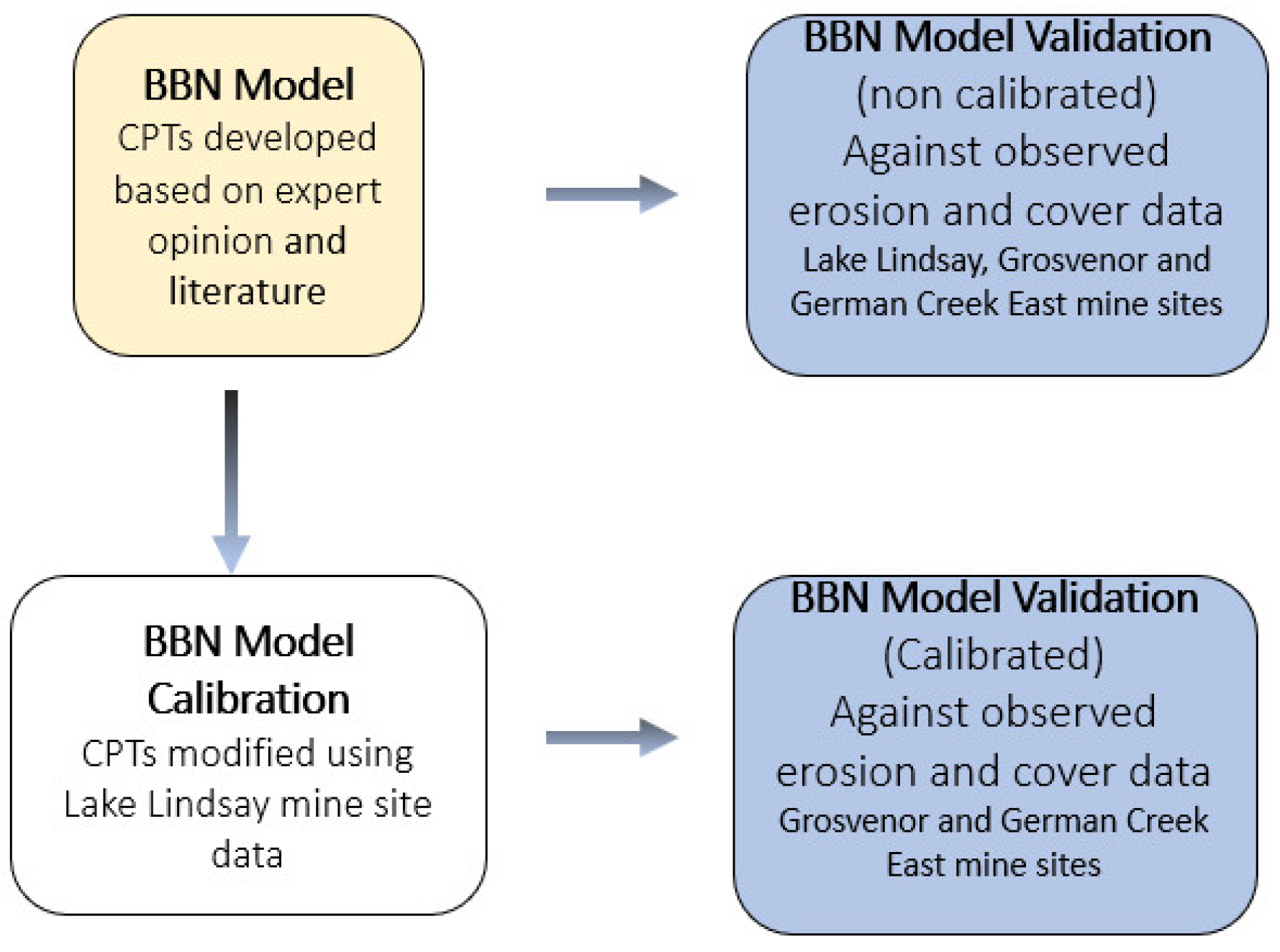
3.3.3. Model Validation
3.4. Field Trials–Data Collection for Model Validation
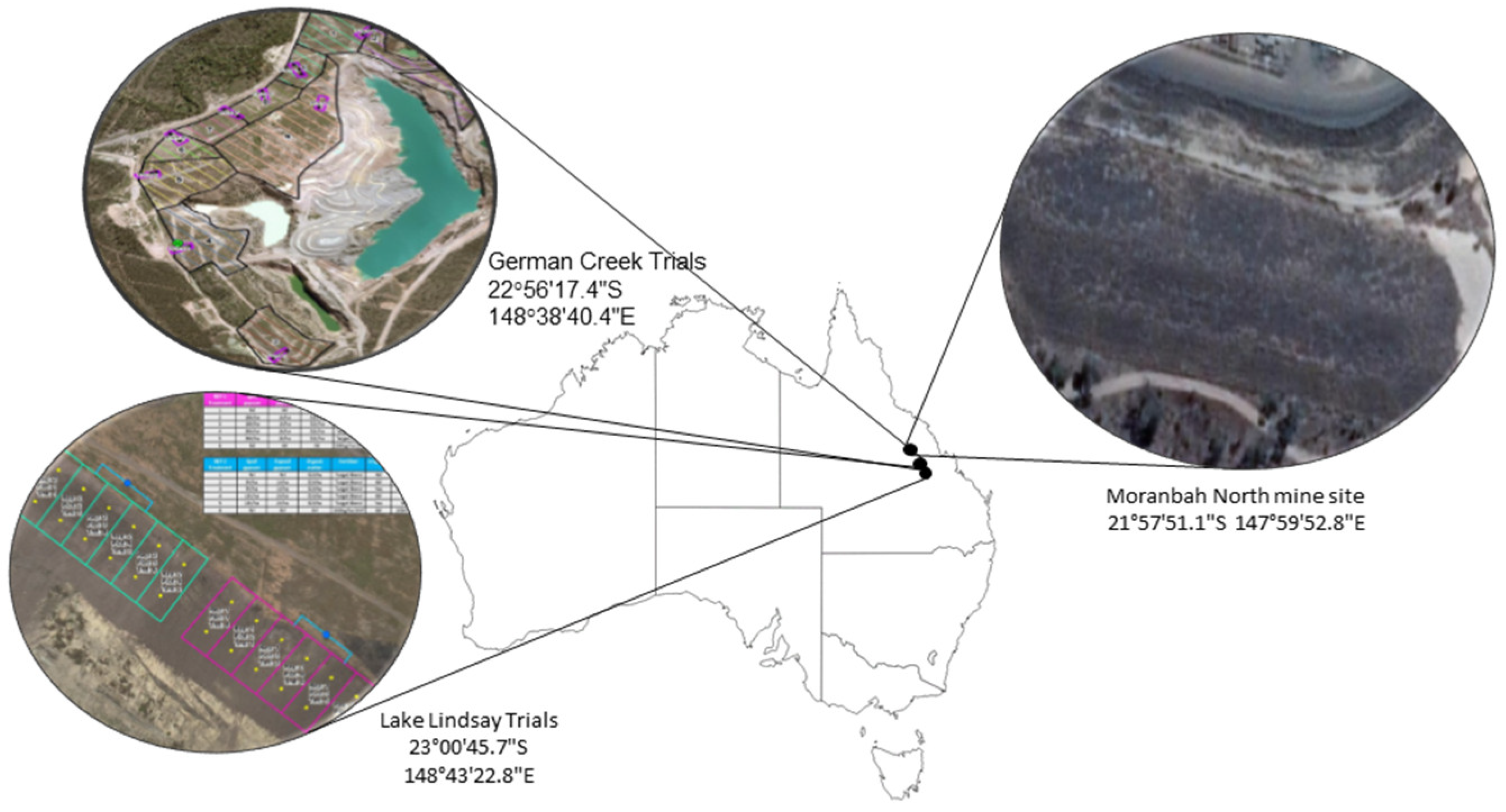
3.4.1. Lake Lindsay
- (a)
- Ripping of spoil (pre-topsoiling) to a depth of 20 cm;
- (b)
- Application of topsoil to a depth of 15 cm;
- (c)
- Incorporation of organic matter into the topsoil at a rate of 52 t/ha (to achieve a target organic matter content of 2%);
- (d)
- Application of a custom fertiliser blend to address all identified nutrient deficiencies;
- (e)
- Cultivation of topsoil (post fertiliser, organic matter and, where relevant, gypsum, to a depth of 15 cm; and
- (f)
- Application of a successional seed mix at the rate of 42 kg/ha.
3.4.2. German Creek East
- (a)
- rock mulch to 500 mm;
- (b)
- rock mulch to 250 mm;
- (c)
- rock mulch to 100 mm with gypsum; and
- (d)
- contour benching with rock-lined drains.
3.4.3. Moranbah North
3.5. Updating of CPTs
- Layer 1 Calcium amount
- Layer 1 Exchangeable dispersion percentage
- Layer 1 Calcium availability
- Topsoil organic matter
- Nutrition
- Surface Gullying Exposure
- Erosion Risk
- Vegetation Cover
- Layer 2 Calcium amount
- Layer 2 Exchangeable dispersion percentage
4. Results and Discussion
4.1. Dispersive Spoil Risk Management–The BBN Framework
4.2. BBN Model Validation
4.3. Scenario Analysis
- Investigation of the impact of site-specific weather and crop scenarios and their effects on soil water storage and erosion risk to inform business discussions, planning and decisions;
- Guidance on the collection of site condition monitoring data;
- Objective guidance for investment in site soil/spoil management;
- Use as a learning and discussion tool when there are limited local data.
4.4. Further Refinement of the BBN Model
4.5. Limitations and Opportunities of Bayesian Belief Networks
5. Conclusions
Supplementary Materials
Author Contributions
Funding
Institutional Review Board Statement
Informed Consent Statement
Data Availability Statement
Acknowledgments
Conflicts of Interest
References
- Vacher, C.A.; Loch, R.J.; Raine, S.R. Identification and Management of Dispersive Mine Spoils. Final Report. Brisbane QLD 2004, Australia: Australian Centre for Mining Environmental Research. Available online: https://eprints.usq.edu.au/1311 (accessed on 29 August 2017).
- Bennett, J.M.; Melland, A.R.; Eberhard, J.; Paton, C.; Clewett, J.F.; Newsome, T.; Baillie, C. Rehabilitating open-cut coal mine spoil for a pasture system in south east Queensland, Australia: Abiotic soil properties compared with unmined land through time. Geoderma Reg. 2021, 25, e00364. [Google Scholar] [CrossRef]
- Baker, P.; Henderson, S.; Grace, D.; Hemsworth, S. Rehabilitation of Highwalls; ACARP Project C14048; ACARP: Brisbane, QLD, Australia, 2006. [Google Scholar]
- Carroll, C.; Pink, L.; Griffiths, S.; Tucker, A.; Burger, P.; Merton, L.; Cameron, D. Long Term Erosion and Water Quality Assessment from a Range of Coal Mine Rehabilitation Practices; ACARP study C10037; ACARP: Brisbane, QLD, Australia, 2004. [Google Scholar]
- Dale, G.T.; Reardon-Smith, K.; Bennett, J.M.C.L.; Thomas, E.; McCallum, L.; Raine, S. A process-based approach to mine rehabilitation decision making illustrated through Bayesian modelling and a risk-based approach to practices for dispersive spoil rehabilitation. In Proceedings of the 12th International Conference on Mine Closure, Leipzig, Germany, 3–7 September 2018; pp. 435–446. [Google Scholar]
- Dale, G.; Thomas, E.; McCallum, L.; Raine, S.R.; Bennett, J.M.; Reardon-Smith, K. Applying Risk-Based Principles of Dispersive Mine Spoil Behaviour to Facilitate Development of Cost-Effective Best Management Practices; ACARP Project C24033; University of Southern Queensland and Verterra: Brisbane, QLD, Australia, 2018. [Google Scholar]
- Loch, R.J. Sustainable Landscape Design for Coal Mine Rehabilitation; ACARP project C18024; ACARP: Brisbane, QLD, Australia, 2010; 94p. [Google Scholar]
- So, H.B.; Aylmore, L.A.G. How do sodic soils behave-the effects of sodicity on soil physical behavior. Soil Res. 1993, 31, 761–777. [Google Scholar] [CrossRef]
- Qadir, M.; Schubert, S. Degradation processes and nutrient constraints in sodic soils. Land. Degrad. Dev. 2002, 13, 275–294. [Google Scholar] [CrossRef]
- Minserve Group. Rehabilitation of Dispersive Tertiary Spoil in the Bowen Basin. ACARP Project C12031. Brisbane QLD 2004, Australia: Australian Coal Research Limited. Available online: http://www.acarp.com.au/abstracts.aspx?repId=C12031 (accessed on 29 August 2017).
- Bennett, J.M.; Marchuk, A.; Marchuk, S.; Raine, S.R. Towards predicting the soil-specific threshold electrolyte concentration of soil as a reduction in saturated hydraulic conductivity: The role of clay net negative charge. Geoderma 2019, 337, 122–131. [Google Scholar] [CrossRef]
- Zhu, Y.; Ali, A.; Dang, A.; Wandel, A.P.; Bennett, J.M. Re-examining the flocculating power of sodium, potassium, magnesium and calcium for a broad range of sssoils. Geoderma 2019, 352, 422–428. [Google Scholar] [CrossRef]
- Schreiber, E.S.G.; Bearlin, A.R.; Nicol, S.J.; Todd, C.R. Adaptive management: A synthesis of current understanding and effective application. Ecol. Manag. Restor. 2004, 5, 177–182. [Google Scholar] [CrossRef]
- Howard, E.J.; Loch, R.J.; Vacher, C.A. Evolution of landform design concepts. Min. Technol. 2011, 120, 112–117. [Google Scholar] [CrossRef]
- DEHP (Department of Environment and Heritage Protection), Rehabilitation Requirements for Mining Resource Activities. Brisbane QLD 2014, Australia: Department of Environment and Heritage Protection (DEHP). Available online: https://www.ehp.qld.gov.au/assets/documents/regulation/rs-gl-rehabilitation-requirements-mining.pdf (accessed on 29 August 2017).
- Moore, G.A. Soilguide (Soil Guide): A Handbook for Understanding and Managing Agricultural Soils; Department of Agriculture, Western Australia: Perth, WA, Australia, 2001. [Google Scholar]
- Bennett, J.; Raine, S.; Reardon-Smith, K.; Dale, G.; Thomas, E. Applying Risk-Based Principles of Dispersive Mine Spoil Behaviour to Facilitate Development of Cost-Effective Best Management Practices; Report prepared for Verterra and the Australian Coal Association Research Program; Institute for Agriculture and the Environment (IAgE) 2017, University of Southern Queensland: Toowoomba, QLD, Australia, 2017. [Google Scholar]
- Farmani, R.; Henriksen, H.J.; Savic, D.; Butler, D. An evolutionary Bayesian belief network methodology for participatory decision making under uncertainty: An application to groundwater management. Integr. Environ. Assess. 2012, 8, 456–461. [Google Scholar] [CrossRef]
- Roberton, S.D.; Bennett, J.M.; Lobsey, C.R.; Bishop, T.F. Assessing the Sensitivity of Site-Specific Lime and Gypsum Recommendations to Soil Sampling Techniques and Spatial Density of Data Collection in Australian Agriculture: A Pedometric Approach. Agronomy 2020, 10, 1676. [Google Scholar] [CrossRef]
- Pollino, C.A.; Hart, B.T.; Bolton, B.R. Modelling ecological risks from mining activities in a tropical system. Australas. J. Ecotoxicol. 2008, 14, 119. [Google Scholar]
- Pollino, C.A.; Henderson, C. Bayesian Networks: A Guide for Their Application in Natural Resource Management and Policy. Landscape Logic 2010, Technical Report, 14. Available online: http://www.utas.edu.au/__data/assets/pdf_file/0009/588474/TR_14_BNs_a_resource_guide.pdf (accessed on 1 August 2021).
- Marcot, B.G.; Penman, T.D. Advances in Bayesian network modelling: Integration of modelling technologies. Environ. Modell. Softw. 2019, 111, 386–393. [Google Scholar] [CrossRef]
- Obeng-Gyasi, E.; Roostaei, J.; Gibson, J.M. Lead Distribution in Urban Soil in a Medium-Sized City: Household-Scale Analysis. Environ. Sci. Technol. 2021, 55, 3696–3705. [Google Scholar] [CrossRef] [PubMed]
- Ghahramani, A.; Freebairn, D.M.; Sena, D.R.; Cutajar, J.L.; Silburn, D.M. A pragmatic parameterisation and calibration approach to model hydrology and water quality of agricultural landscapes and catchments. Environ. Model. Softw. 2020, 130, 104733. [Google Scholar] [CrossRef]
- Borusk, M.E.; Stow, C.A.; Reckhow, K.H. A Bayesian network of eutrophication models for synthesis, prediction, and uncertainty analysis. Ecol. Model. 2004, 173, 219–239. [Google Scholar] [CrossRef]
- Fenton, N.; Neil, M. Risk Assessment and Decision Analysis with Bayesian Networks; CRC Press: Boca Raton, FL, USA, 2018. [Google Scholar]
- Guan, L.; Liu, Q.; Abbasi, A.; Ryan, M.J. Developing a comprehensive risk assessment model based on fuzzy Bayesian belief network (FBBN). J. Constr. Eng. Manag. 2020, 26, 614–634. [Google Scholar] [CrossRef]
- Environmental Protection Agency. Guidance on the Development, Evaluation, and Application of Environmental Models; EPA/100/K-09/003; Environmental Protection Agency: Washington, DC, USA, 2009. [Google Scholar]
- Pollino, C.A.; Woodberry, O.; Nicholson, A.; Korb, K.; Hart, B.T. Parameterisation and evaluation of a Bayesian network for use in an ecological risk assessment. Environ. Modell. Softw. 2007, 22, 1140–1152. [Google Scholar] [CrossRef]
- Bronick, C.J.; Lal, R. Soil structure and management: A reviesw. Geoderma 2005, 124, 3–22. [Google Scholar] [CrossRef]
- Letcher, R.A.; Jakeman, A.J.; Croke, B.F.W. Model development for integrated assessment of water allocation options. Water Resour. Res. 2004, 40. [Google Scholar] [CrossRef] [Green Version]
- Trucco, P.; Cagno, E.; Ruggeri, F.; Grande, O. A Bayesian Belief Network modelling of organisational factors in risk analysis: A case study in maritime transportation. Reliab. Eng. Syst. Safe 2008, 93, 845–856. [Google Scholar] [CrossRef]
- Troldborg, M.; Aalders, I.; Towers, W.; Hallett, P.D.; McKenzie, B.M.; Bengough, A.G.; Lilly, A.; Ball, B.C.; Hough, R.L. Application of Bayesian Belief Networks to quantify and map areas at risk to soil threats: Using soil compaction as an example. Soil Till. Res. 2013, 132, 56–68. [Google Scholar] [CrossRef]
- Norsys Software Corp., 1992–2017. NeticaTM Application. A complete software package to solve problems using Bayesian belief networks and influence diagrams. Version 6.02. Norsys Software Corporation: Vancouver, BC, Canada. Available online: https://www.norsys.com/about_us.htm(accessed on 1 August 2021).
- Wischmeier, W.H.; Smith, D.D. Predicting Rainfall Erosion Losses: A Guide to Conservation Planning (No. 537); Department of Agriculture Science and Education Administration: Washington, DC, USA, 1978. [Google Scholar]
- Crouch, R.J. Field tunnel erosion—A review. J. Soil Conserv. N. South Wales 1976, 32, 98–111. [Google Scholar]
- Williams, B.K.; Johnson, F.A. Frequencies of decision making and monitoring in adaptive resource management. PLoS ONE 2017, 12. [Google Scholar] [CrossRef] [Green Version]
- Koch, A.; McBratney, A.; Adams, M.; Field, D.; Hill, R.; Crawford, J.; Minasny, B.; Lal, R.; Abbott, L.; O’Donnell, A.; et al. Soil security: Solving the global soil crisis. Glob. Policy 2013, 4, 434–441. [Google Scholar] [CrossRef] [Green Version]
- Horton, R.E. The role of infiltration in the hydrologic cycle. Eos Trans. Am. Geophys. Union 1933, 14, 446–460. [Google Scholar] [CrossRef]
- Ghahramani, A.; Ishikawa, Y.; Gomi, T.; Miyata, S. Downslope soil detachment–transport on steep slopes via rain splash. Hydrol. Process. 2011, 25, 2471–2480. [Google Scholar] [CrossRef]
- Ghahramani, A.; Ishikawa, Y.; Gomi, T.; Shiraki, K.; Miyata, S. Effect of ground cover on splash and sheetwash erosion over a steep forested hillslope: A plot-scale study. Catena 2011, 85, 34–47. [Google Scholar] [CrossRef]
- Smith, C.S.; Howes, A.L.; Price, B.; McAlpine, C.A. Using a Bayesian belief network to predict suitable habitat of an endangered mammal–The Julia Creek dunnart (Sminthopsis douglasi). Biol. Conserv. 2007, 139, 333–347. [Google Scholar] [CrossRef]
- Hardie, M.A.; Cotching, W.E.; Zund, P.R. Rehabilitation of field tunnel erosion using techniques developed for construction with dispersive soils. Soil Res. 2007, 45, 280–287. [Google Scholar] [CrossRef]
- Bennett, J.M.; Marchuk, A.; Marchuk, S. An alternative index to the exchangeable sodium percentage for an explanation of dispersion occurring in soils. Soil Res. 2016, 54, 949–957. [Google Scholar] [CrossRef]
- Rengasamy, P.; Marchuk, A. Cation ratio of soil structural stability (CROSS). Soil Res. 2011, 49, 280–285. [Google Scholar] [CrossRef]
- Dang, A.; Bennett, J.M.; Marchuk, A.; Biggs, A.; Raine, S.R. Quantifying the aggregation-dispersion boundary condition in terms of saturated hydraulic conductivity reduction and the threshold electrolyte concentration. Agr. Water. Manag. 2018, 203, 172–178. [Google Scholar] [CrossRef]
- Quirk, J.P.; Schofield, R.K. The effect of electrolyte concentration on soil permeability. J. Soil Sci. 1955, 6, 163–178. [Google Scholar] [CrossRef]
- Bennett, J.M.; Cattle, S.; Singh, B. The Efficacy of Lime, Gypsum and Their Combination to Ameliorate Sodicity in Irrigated Cropping Soils in the Lachlan Valley of New South Wales. Arid. Land. Res. Manag. 2015, 29, 17–40. [Google Scholar] [CrossRef]
- Ali, A.; Biggs, A.J.; Marchuk, A.; Bennett, J.M. Effect of irrigation water pH on saturated hydraulic conductivity and electrokinetic properties of acidic, neutral, and alkaline soils. Soil Sci. Soc. Am. J. 2019, 83, 1672–1682. [Google Scholar] [CrossRef]
- Ali, A.; Biggs, A.J.; Šimůnek, J.; Bennett, J.M. A pH-Based Pedotransfer Function for Scaling Saturated Hydraulic Conductivity Reduction: Improved Estimation of Hydraulic Dynamics in HYDRUS. Vadose. Zone J. 2019, 18, 190072. [Google Scholar] [CrossRef]
- Bennett, J.M.; McKenzie, D.C.; Ali, A.; Biggs, A.; Birchall, C.; Flavel, R.J.; Ghahramani, A.; Guppy, C.N.; Hill, J.V.; Knox, O.; et al. Submitted. On the importance of soil stability functional assessment. Geoderma 2021, 385. [Google Scholar]
- Chorom, M.; Rengasamy, P.; Murray, R.S. Clay dispersion as influenced by pH and net particle charge of sodic soils. Soil Res. 1994, 32, 1243–1252. [Google Scholar] [CrossRef]
- Hazelton, P.; Murphy, B. Interpreting Soil Test Results: What Do All the Numbers Mean? CSIRO Publishing: Clayton South, VIC, Australia, 2016. [Google Scholar]
- Hsu, W.; Bui, A.A. Disease Models, Part II: Querying & Applications. In Medical Imaging Informatics; Springer: Boston, MA, USA, 2010; pp. 371–401. [Google Scholar]
- Kleemann, J.; Celio, E.; Fürst, C. Validation approaches of an expert-based Bayesian belief network in Northern Ghana, West Africa. Ecol. Model. 2017, 365, 10–29. [Google Scholar] [CrossRef]
- Dang, K.B.; Windhorst, W.; Burkhard, B.; Müller, F. A Bayesian Belief Network–Based approach to link ecosystem functions with rice provisioning ecosystem services. Ecol. Indic. 2019, 100, 30–44. [Google Scholar] [CrossRef]
- Rohmer, J. Uncertainties in conditional probability tables of discrete Bayesian Belief Networks: A comprehensive review. Eng. Appl. Artif. Intell. 2020, 88, 103384. [Google Scholar] [CrossRef] [Green Version]
- Zhou, Y.; Fenton, N.; Neil, M. Bayesian network approach to multinomial parameter learning using data and expert judgments. Int. J. Approx. Reason. 2014, 55, 1252–1268. [Google Scholar] [CrossRef]
- Lang, R.D.; McCaffrey, L.A.H. Ground cover—Its affects on soil loss from grazed runoff plots, Gunnedah. J. Soil Conserv. Serv. N. S. W. 2013, 40, 56. [Google Scholar]
- Evans, K.G. Methods for assessing mine site rehabilitation design for erosion impact. Soil Res. 2000, 38, 231–248. [Google Scholar] [CrossRef]
- Hancock, G.R.; Verdon-Kidd, D.; Lowry, J.B.C. Soil erosion predictions from a landscape evolution model–An assessment of a post-mining landform using spatial climate change analogues. Sci. Total Environ. 2017, 601, 109–121. [Google Scholar] [CrossRef] [PubMed]
- Rose, C.W.; Williams, J.R.; Sander, G.C.; Barry, D.A. A Mathematical Model of Soil Erosion and Deposition Processes: I. Theory for a Plane Land Element. Soil Sci. Soc. Am. J. 1983, 47, 991–995. [Google Scholar] [CrossRef]
- Gregory, R.; Ohlson, D.; Arvai, J. Deconstructing adaptive management: Criteria for applications to environmental management. Ecol. Appl. 2006, 16, 2411–2425. [Google Scholar] [CrossRef] [Green Version]
- Greene, R.S.B.; Ford, G.W. The effect of gypsum on cation exchange in two red duplex soils. Soil Res. 1985, 23, 61–74. [Google Scholar] [CrossRef]
- Miller, C.J.; Yesiller, N.; Yaldo, K.; Merayyan, S. Impact of Soil Type and Compaction Conditions on Soil Water Characteristic. J. Geotech. Geoenviron. 2002, 128, 733–742. [Google Scholar] [CrossRef]
- Drescher, M.; Perera, A.H.; Johnson, C.J.; Buse, L.J.; Drew, C.A.; Burgman, M.A. Toward rigorous use of expert knowledge in ecological research. Ecosphere 2013, 4, 1–26. [Google Scholar] [CrossRef]
- Anderson, J.L. Embracing uncertainty: The interface of Bayesian statistics and cognitive pschology. Conserv. Ecol. 1998, 2. [Google Scholar] [CrossRef] [Green Version]
- Baddeley, M.; Curtis, A.; Wood, R. An introduction to prior information derived from probabilistic judgements: Elicitation of knowledge, cognitive bias and herding. Geol. Soc. Lond. Spec. Publ. 2004, 239, 15–27. [Google Scholar] [CrossRef] [Green Version]
- Burgman, M. Risks and Decisions for Conservation and Environmental Management; Cambridge University Press: Cambridge, UK, 2005. [Google Scholar]

| Site | No Trials | Treatments | Observed Gully Erosion% | Predicted Erosion Risk from BBN Model | |||
|---|---|---|---|---|---|---|---|
| Low | Medium | High | Very High | ||||
| Lake Lindsay | 1 | Gypsum 2 & Dry | 0.0 | 32.1 | 23.7 | 21.6 | 22.6 |
| 2 | Gypsum 1& Irrig. | 0.0 | 32.0 | 23.8 | 21.3 | 22.9 | |
| 3 | Rock mulch | 0.0 | 26.6 | 23.2 | 22.3 | 27.9 | |
| 4 | Gypsum 1 & Dry | 1.7 | 32.1 | 23.7 | 21.6 | 22.6 | |
| 5 | Gypsum 2 & Dry | 20.3 | 29 | 23.8 | 22.4 | 24.8 | |
| 6 | Control | 0.0 | 28.8 | 23.8 | 22.4 | 25 | |
| 7 | Gypsum 1 & Irrig. | 0.0 | 29.4 | 23.8 | 22.2 | 24.6 | |
| 8 | Rock mulch | 0.0 | 46.5 | 21.8 | 17.9 | 13.8 | |
| 9 | Gypsum 2 & Irrig. | 18.2 | 50.8 | 21.3 | 16.6 | 11.3 | |
| 10 | Gypsum 1 & Dy | 12.7 | 49.9 | 21.6 | 17 | 11.5 | |
| 11 | Control- | 0.0 | 50.3 | 21.5 | 16.8 | 11.4 | |
| 12 | Gypsum 2 & Irrig. | 0.0 | 50.4 | 21.4 | 16.8 | 11.4 | |
| 13 | Gypsum 2 & Dry | 0.0 | 56.6 | 19.1 | 14.5 | 9.8 | |
| 14 | Gypsum 1 & Irrig. | 0.0 | 54.7 | 19.9 | 15.2 | 10.3 | |
| 15 | Rock mulch | 0.0 | 46.5 | 21.7 | 17.9 | 13.8 | |
| 16 | Gypsum 1 & Dry | 0.0 | 44.1 | 22.6 | 18.7 | 14.6 | |
| 17 | Gypsum 2 & Dry | 10.5 | 51.2 | 21.1 | 16.5 | 11.2 | |
| 18 | Control | 1.4 | 54.7 | 19.8 | 15.2 | 10.3 | |
| 19 | Rock mulch | 0.0 | 38 | 23.3 | 20.5 | 18.2 | |
| 20 | Gypsum 2 &s Irrig. | 0 | 54.7 | 19.8 | 15.2 | 10.3 | |
| Moranbah North | 1 | No treatment | NIL | 32.1 | 23.6 | 21.7 | 22.6 |
| 2 | No treatment | NIL | 39.7 | 22.8 | 19.7 | 17.8 | |
| 3 | No treatment | NIL | 46.7 | 21.7 | 17.7 | 14 | |
| 4 | No treatment | NIL | 45.4 | 22s | 18.1 | 14.4 | |
| 5 | No treatment | NIL | 49.5 | 20.7 | 16.7 | 13.1 | |
| 6 | No treatment | NIL | 48 | 21.2 | 17.2 | 13.6 | |
| 7 | No treatment | NIL | 46.3 | 21.7 | 17.8 | 14.2 | |
| 8 | No treatment | NIL | 45 | 22.1 | 18.2 | 14.6 | |
| German Creek East | 1 | Full rock (500 mm) | 0 | 24.9 | 23.2 | 22.7 | 29.2 |
| 2 | Full rock (500 mm) | 0 | 29.4 | 24 | 22.4 | 24.2 | |
| 3 | Gypsum & 100 mm rock | 0 | 27.1 | 23.3 | 22.3 | 27.4 | |
| 4 | Gypsum & 100 mm rock | 0 | 22.1 | 22.4 | 22.5 | 33 | |
| 5 | Contour benching & rock drains | 5.4 | 27.1 | 23.5 | 22.5 | 26.9 | |
| 6 | Contour benching & rock drains | 36.8 | 20.5 | 21.8 | 22.4 | 35.3 | |
| 7 | Half rock (250 mm) | 0 | 24.8 | 23.2 | 22.7 | 29.3 | |
| 8 | Half rock (250 mm) | 0 | 55.6 | 19.7 | 14.9 | 9.9 | |
| Site | No Trials | Observed Cover % | Predicted Vegetation Cover% from BBN Mode | ||
|---|---|---|---|---|---|
| Low | Medium | High | |||
| Lake Lindsay | 1 | 0.9 (high) | 16.7 | 39.6 | 43.7 |
| 2 | 1.0 (high) | 12.2 | 40.7 | 47.1 | |
| 3 | 0.6 (Low) | 16.1 | 43.1 | 42.6 | |
| 4 | 0.7 (medium) | 14.3 | 40.8 | 44.9 | |
| 5 | 1.0 (high) | 14.5 | 40.9 | 44.6 | |
| 6 | 0.9 (high) | 16.2 | 41.3 | 42.4 | |
| 7 | 1.0 (high) | 14.4 | 40.9 | 44.7 | |
| 8 | 0.3 (low) | 23.1 | 40.0 | 36.9 | |
| 9 | 0.9 (high) | 14.3 | 40.3 | 45.6 | |
| 10 | 0.9 (high) | 14.5 | 41.0 | 44.4 | |
| 11 | 0.7 (medium) | 16.0 | 41.1 | 42.8 | |
| 12 | 0.9 (high) | 12.5 | 36.1 | 51.4 | |
| 13 | 0.9 (high) | 13.9 | 37.6 | 48.5 | |
| 14 | 0.8 (medium) | 14.1 | 37.4 | 48.5 | |
| 15 | 0.6 (Low) | 15.9 | 38.6 | 45.5 | |
| 16 | 0.6 (Low) | 16.0 | 38.6 | 45.4 | |
| 17 | 0.9 (high) | 13.6 | 37.6 | 48.8 | |
| 18 | 0.7 (medium) | 16.0 | 38.6 | 45.4 | |
| 19 | 0.20 (low) | 20.0 | 37.9 | 42.1 | |
| 20 | 0.9 (high) | 15.7 | 35.1 | 49.2 | |
| 21 | 0.7 (medium) | 15.3 | 35.7 | 49.0 | |
| Moranbah North | 1 | 0.2 (low) | 38.5 | 40.4 | 21.1 |
| 2 | 0.6 (low) | 31.4 | 41.9 | 26.7 | |
| 3 | 0.9 (high) | 32.4 | 41.6 | 25.9 | |
| 4 | 1.0 (high) | 23.2 | 40.8 | 36.0 | |
| 5 | 1.0 (high) | 23.5 | 40.9 | 35.6 | |
| 6 | 1.0 (high) | 20.6 | 41.3 | 38.2 | |
| 7 | 1.0 (high) | 21.9 | 41.0 | 37.0 | |
| 8 | 1.0 (high) | 21.3 | 40.9 | 37.8 | |
| 9 | 1.0 (high) | 18.6 | 40.3 | 41.1 | |
| 10 | 0.9 (high) | 24.0 | 37.7 | 38.3 | |
| 11 | 1.0 (high) | 29.6 | 40.3 | 30.2 | |
| 12 | 0.6 (Low) | 26.5 | 40.6 | 33.2 | |
| German Creek East | 1 | 0.42 (low) | 36.6 | 40.8 | 22.7 |
| 2 | 0.72 (medium) | 28.7 | 40.4 | 30.9 | |
| 3 | 0.29 (low) | 21.8 | 40.0 | 38.2 | |
| 4 | 0.12 (low) | 21.5 | 40.7 | 37.8 | |
| 5 | 0.29 (low) | 28.0 | 40.2 | 31.8 | |
| 6 | 0.13 (low) | 36.6 | 41.2 | 22.1 | |
| 7 | 0.28 (low) | 34.8 | 41.6 | 23.5 | |
| 8 | 0.99 (high) | 29.9 | 42.0 | 28.2 | |
| Site | No Trials | Treatments | Observed Gully Erosion% | Predicted Erosion Risk from Updated BBN Model | |||
|---|---|---|---|---|---|---|---|
| Low | Medium | High | Very High | ||||
| Moranbah North | 1 | No treatment | 0 | 44.3 | 19.9 | 21.7 | 14.1 |
| 2 | No treatment | 0 | 44.5 | 19.9 | 21.6 | 14.0 | |
| 3 | No treatment | 0 | 45.1 | 19.9 | 21.3 | 13.8 | |
| 4 | No treatment | 0 | 50.4 | 19.5 | 18.4 | 11.8 | |
| 5 | No treatment | 0 | 49.3 | 19.7 | 18.9 | 12.1 | |
| 6 | No treatment | 0 | 51.2 | 19.3 | 17.9 | 11.6 | |
| 7 | No treatment | 0 | 47.8 | 19.6 | 19.8 | 12.8 | |
| 8 | No treatment | 0 | 49.8 | 19.4 | 18.7 | 12.1 | |
| 9 | No treatment | 0 | 50.6 | 19.3 | 18.3 | 11.9 | |
| 10 | No treatment | 0 | 50.4 | 19.3 | 18.0 | 12.3 | |
| 11 | No treatment | 0 | 48.9 | 19.4 | 19.2 | 12.5 | |
| 12 | No treatment | 0 | 46.0 | 20.5 | 20.1 | 13.4 | |
| German Creek East | 1 | Full rock (500mm) | 0 | 37.9 | 31.5 | 21.1 | 9.4 |
| 2 | Full rock (500 mm) | 0 | 32.7 | 31.7 | 24.6 | 11.0 | |
| 3 | Gypsum + 100 mm rock | 0 | 30.1 | 32.2 | 26.3 | 11.5 | |
| 4 | Gypsum + 100 mm rock | 0 | 32.9 | 31.6 | 24.6 | 10.9 | |
| 5 | Contour benching w rock drains | 5.4 | 29.8 | 29.9 | 27.7 | 12.6 | |
| 6 | Contour benching w rock drains | 36.8 | 27.0 | 30.3 | 29.6 | 13.2 | |
| 7 | Half rock (250 mm) | 0 | 36.6 | 23.4 | 27.1 | 12.9 | |
| 8 | Half rock (250 mm) | 0 | 49.1 | 19.9 | 21.3 | 9.68 | |
| Site | Soil Sample No. | Observed Cover % | Predicted Vegetation Cover% from Updated BBN Model | ||
|---|---|---|---|---|---|
| Low | Medium | High | |||
| Moranbah North | 1 | 0.2 (low) | 39.6 | 34.9 | 25.5 |
| 2 | 0.6 (low) | 34.3 | 39.5 | 26.2 | |
| 3 | 0.9 (high) | 29.6 | 37.5 | 32.9 | |
| 4 | 1.0 (high) | 13.8 | 33.4 | 52.6 | |
| 5 | 1.0 (high) | 17.5 | 36.2 | 45.9 | |
| 6 | 1.0 (high) | 15.1 | 35.5 | 49.4 | |
| 7 | 1.0 (high) | 25.6 | 35.5 | 38.9 | |
| 8 | 1.0 (high) | 18.4 | 34.1 | 47.5 | |
| 9 | 1.0 (high) | 18.0 | 34.1 | 47.8 | |
| 10 | 0.9 (high) | 18.6 | 34.1 | 47.3 | |
| 11 | 1.0 (high) | 24.3 | 3.9 | 40.8 | |
| German Creek East | 1 | 0.42 (low) | 35.5 | 36.5 | 28.1 |
| 2 | 0.72 (medium) | 35.4 | 36.3 | 28.4 | |
| 3 | 0.29 (low) | 53.3 | 30.6 | 16.1 | |
| 4 | 0.12 (low) | 47.6 | 31.1 | 21.3 | |
| 5 | 0.29 (low) | 45.2 | 32.9 | 21.9 | |
| 6 | 0.13 (low) | 46.5 | 32.2 | 21.3 | |
| 7 | 0.28 (low) | 47.6 | 32.7 | 19.8 | |
| 8 | 0.99 (high) | 27.6 | 36.0 | 36.3 | |
| Node | State | Best Case Probability % | Worst Case Probability % | Node | State | Best Case Probability % | Worst Case Probability % |
|---|---|---|---|---|---|---|---|
| Surface erosion risk | low | 100 | 0 | Woody species cover | low | 19.0 | 32.2 |
| medium | 0 | 0 | moderate | 31.6 | 33.9 | ||
| high | 0 | 100 | high | 49.4 | 33.9 | ||
| Spoil L1 vulnerability | low | 50.9 | 8.76 | Tunnelling risk | low | 29.7 | 18.2 |
| moderate | 27.7 | 15.3 | medium | 22.6 | 18.6 | ||
| high | 14.8 | 27.4 | high | 21.9 | 19.6 | ||
| very high | 6.66 | 48.6 | v high | 25.8 | 43.6 | ||
| Surface gullying exposure | nil | 67.7 | 18.5 | Runoff risk | very low | 22.3 | 17.3 |
| low | 19.7 | 16.9 | low | 31.6 | 26.2 | ||
| moderate | 9.19 | 27.3 | medium | 28.8 | 28.4 | ||
| high | 3.41 | 37.3 | high | 17.4 | 28.1 | ||
| Profile vulnerability | low | 49.9 | 18.0 | Spoil L3 vulnerability | low | 30.4 | 22.9 |
| medium | 18.6 | 16.8 | moderate | 22.4 | 22.3 | ||
| high | 16.1 | 18.9 | high | 22.2 | 23.3 | ||
| very high | 15.4 | 46.4 | very high | 25.0 | 31.5 | ||
| Runoff risk with surface management | very low | 41.8 | 21.7 | Spoil L2 vulnerability | low | 34.4 | 16.2 |
| low | 25.6 | 17.5 | moderate | 24.9 | 21.8 | ||
| medium | 18.1 | 23.4 | high | 22.7 | 24.6 | ||
| high | 14.5 | 37.3 | very high | 18.0 | 37.4 | ||
| Vegetation root depth | shallow | 23.7 | 42.8 | Vegetation cover | low | 27.4 | 41.7 |
| medium | 24.4 | 24.4 | moderate | 36.2 | 35.3 | ||
| deep | 51.9 | 32.8 | high | 36.4 | 23.0 | ||
| Depth of L1 | shallow | 27.7 | 40.0 | Contour bank interval | low | 44.7 | 30.4 |
| moderate | 33.0 | 33.3 | medium | 39.4 | 42.1 | ||
| deep | 39.2 | 26.8 | high | 15.9 | 27.5 | ||
| Zeta potential (L1) | high | 22.6 | 31.6 | Water holding capacity (L1) | low | 51.6 | 63.5 |
| medium | 34.6 | 37.9 | mid | 22.7 | 18.5 | ||
| low | 42.9 | 30.5 | high | 25.7 | 18.0 | ||
| Average annual rainfall | very low | 17.2 | 23.5 | Spoil dispersivity (L1) | low | 46.4 | 25.6 |
| low | 18.7 | 21.6 | moderate | 20.1 | 19.9 | ||
| mid | 20.2 | 19.6 | high | 11.4 | 16.1 | ||
| high | 21.3 | 18.3 | very high | 22.2 | 38.4 | ||
| very high | 22.6 | 16.9 |
| Node | State | Best Case Probability % | Worst Case Probability % |
|---|---|---|---|
| Tunnelling risk | low | 100 | 0 |
| medium | 0 | 0 | |
| high | 0 | 0 | |
| very high | 0 | 100 | |
| Tunnel exposure | none | 50.2 | 4.91 |
| low | 20.6 | 6.09 | |
| medium | 8.27 | 8.29 | |
| high | 20.9 | 80.7 | |
| Profile vulnerability | low | 58.8 | 10.5 |
| medium | 21.7 | 11.4 | |
| high | 12.1 | 21.8 | |
| very high | 7.35 | 56.3 | |
| Ponding | yes | 22.7 | 75.7 |
| no | 77.3 | 24.3 | |
| Spoil L1 vulnerability | low | 43.5 | 14.2 |
| moderate | 26.6 | 19.8 | |
| high | 18.9 | 26.9 | |
| very high | 11.1 | 39.1 | |
| Spoil L2 vulnerability | low | 36.5 | 14.0 |
| moderate | 26.5 | 20.3 | |
| high | 21.5 | 26.1 | |
| very high | 15.6 | 39.6 | |
| Erosion risk | low | 47.8 | 29.6 |
| medium | 20.8 | 23.7 | |
| high | 17.1 | 22.2 | |
| very high | 14.3 | 24.5 | |
| Spoil L3 vulnerability | low | 32.8 | 20.4 |
| moderate | 23.6 | 21.0 | |
| high | 21.6 | 23.8 | |
| very high | 22.0 | 34.8 | |
| Spoil dispersivity (L1) | low | 43.1 | 29.0 |
| mid | 20.3 | 20.2 | |
| high | 12.1 | 15.4 | |
| very high | 24.5 | 35.4 | |
| Upslope bund | yes | 72.9 | 85.0 |
| no | 27.1 | 15.0 | |
| Depth of L1 | shallow | 27.7 | 39.6 |
| moderate | 33.4 | 33.0 | |
| deep | 38.9 | 27.3 | |
| Vegetation root depth | shallow | 27.1 | 38.0 |
| medium | 24.7 | 24.6 | |
| deep | 48.2 | 37.4 | |
| Water holding capacity (L1) | low | 51.8 | 63.0 |
| medium | 22.7 | 18.7 | |
| high | 25.4 | 18.4 |
Publisher’s Note: MDPI stays neutral with regard to jurisdictional claims in published maps and institutional affiliations. |
© 2021 by the authors. Licensee MDPI, Basel, Switzerland. This article is an open access article distributed under the terms and conditions of the Creative Commons Attribution (CC BY) license (https://creativecommons.org/licenses/by/4.0/).
Share and Cite
Ghahramani, A.; Bennett, J.M.; Ali, A.; Reardon-Smith, K.; Dale, G.; Roberton, S.D.; Raine, S. A Risk-Based Approach to Mine-Site Rehabilitation: Use of Bayesian Belief Network Modelling to Manage Dispersive Soil and Spoil. Sustainability 2021, 13, 11267. https://doi.org/10.3390/su132011267
Ghahramani A, Bennett JM, Ali A, Reardon-Smith K, Dale G, Roberton SD, Raine S. A Risk-Based Approach to Mine-Site Rehabilitation: Use of Bayesian Belief Network Modelling to Manage Dispersive Soil and Spoil. Sustainability. 2021; 13(20):11267. https://doi.org/10.3390/su132011267
Chicago/Turabian StyleGhahramani, Afshin, John McLean Bennett, Aram Ali, Kathryn Reardon-Smith, Glenn Dale, Stirling D. Roberton, and Steven Raine. 2021. "A Risk-Based Approach to Mine-Site Rehabilitation: Use of Bayesian Belief Network Modelling to Manage Dispersive Soil and Spoil" Sustainability 13, no. 20: 11267. https://doi.org/10.3390/su132011267
APA StyleGhahramani, A., Bennett, J. M., Ali, A., Reardon-Smith, K., Dale, G., Roberton, S. D., & Raine, S. (2021). A Risk-Based Approach to Mine-Site Rehabilitation: Use of Bayesian Belief Network Modelling to Manage Dispersive Soil and Spoil. Sustainability, 13(20), 11267. https://doi.org/10.3390/su132011267