Abstract
Window energy consumption has become a key factor in designing buildings with optimal energy efficiency. To that end, herein, the use of an energy-saving insulated window (ESIW) is proposed, particularly for winter heat conservation. DeST software was used to evaluate the energy consumption properties of a house with an ESIW-structure window, as well as that of six other window structures currently on the market. The results were subsequently compared. Furthermore, a series of numerical simulations were carried out using Airpak software to investigate the insulation performance of four ESIW models (A, B, C, and D) under different influencing factors. Finally, the response surface method (RSM) was used to obtain the optimal ESIW structure installation conditions and the weight of each factor. The data shows that houses with ESIW-structure windows exhibit a more suitable indoor natural temperature; less heating load, cooling load, and cumulative annual load; and a more feasible price–load ratio than other energy-saving windows. Furthermore, the average temperature gradually decreased in response to decreasing the electric heater power and energy-saving standard, and increasing the heat transfer coefficient (HTC) and window-to-wall ratio (WWR). Thus, as the energy-saving standard (ESS) increases, the importance of the WWR increases in parallel. This study puts forward an HTC prediction formula that is applicable to different conditions. The optimal thermal efficiency conditions consisted of HTC = 1.07 W/m2 × K, WWR = 0.26, and an ESS of 75%. This study demonstrates that the ESIW system has optimal energy-saving properties and broad adaptability and operability, which can be applied in building insulation as a key insulation component.
1. Introduction
1.1. Research Background
Due to rapid urbanization and improvements in the living standard, building energy consumption in China has drastically increased, and now accounts for nearly 40% of society’s overall energy use [1,2]. Windows are an extremely important building element, as they provide daylight, ventilation, and outdoor views for the occupants, all of which have proven to be essential for human health. However, previous studies have shown that nearly 40% of a building’s total thermal loss is due to exterior windows [3,4,5]. Thus, because of their poor thermal insulation performance, windows are generally considered a major source of heat loss in buildings. As such, improving the insulation performance of external windows has the potential to significantly reduce building energy use.
1.2. Literature Review
Numerous research investigations have been conducted on energy-saving windows. Cuce et al. [6] constructed a test rig consisting of four different glazing configurations with the same thickness and determined the overall heat transfer coefficient (HTC; U-value) of each sample in an environmental chamber. Gao et al. [7] assembled light diffusing and thermal insulating aerogel glazing units (AGUs) by incorporating small or large silica aerogel granules, respectively, into the cavity of double-glazed units. Subsequently, he compared the effect of aerogel granule size on heat loss reduction and light transmittance. Because aerogel is characterized by high surface area, low density, open pore structure, and excellent insulation properties, Cha et al. [8] experimented with using it to reduce the window’s overall HTC. Alfano et al. [9] presented the experimental results from air-tightness measurements carried out using the fan pressurization method in three residential buildings before and after a window retrofit, and Yoo et al. [10] measured the thermal performance (U-factor) of different window systems and analyzed their effects on energy savings.
In addition, Lee et al. [11] evaluated large-area polymer thermochromic (TC) laminated windows in a full-scale testbed office. Because a high visible transmittance in both the switched and unswitched state is also desirable to reduce lighting energy use and enhance indoor environmental quality, Ye et al. [12] discussed the energy saving performance and corresponding theoretical limitations of active/passive smart windows regulating solar spectrum response properties using the energy consumption index. An et al. [13] analyzed the heating and cooling performance of an office building equipped with amorphous-Si (a-Si), building-integrated photovoltaic (BIPV) windows, and Buratti et al. [14] constructed four samples consisting of either float or low emissivity (Low-E) glasses, and granular or monolithic aerogel in the interspace, then measured the samples’ main optical characteristics. Gasparella et al. [15] selected a well-insulated residential building as their research object, and evaluated the impact of double- and triple-glazed systems, window size, orientation of the main windowed facade, and internal gains on winter and summer energy requirements and peak loads. Amirkhani et al. [16] investigated the impact of a specific type of Low-E window film on the holistic energy consumption of an existing hotel building.
Other proposed sophisticated technologies include triple-glazing technology [17], external solar shading screens [18], doubled glazed window combined with light colored walls and roofs [19], natural ventilation [20], indoor thermal environments [21], Parallel Slat Transparent Insulation Material (PS-TIM) systems [22], window-opening behavior [23], impact of energy retrofits [24], translucent solar walls [25], active/passive ventilation walls [26], and windows with photovoltaic (PV) technology, aerogel glazing, or phase change material (PCM) glazing [27,28,29,30,31]. These methods are very efficient for satisfying building envelope thermal regulations, but they substantially deteriorate the view and reduce the occupants’ thermal comfort. Other smart windows also serve as good thermal insulators, but their high manufacturing cost inhibits large-scale commercialization.
1.3. Research Aims and Contents
Previous studies have primarily focused on improving window absolute heat insulation by thickening the glass or increasing the number of glass pieces. While multilayer glazing offers excellent overall insulation performance, especially when integrated with low-E coatings, it results in thicker and heavier constructions, which are undesirable with respect to design and aesthetics. Furthermore, the HTC tends to stop decreasing after the insulation layer reaches a certain thickness.
Likewise, adding an air, inert gas, or a vacuum layer between the glass pieces to “mechanically” reduce the total HTC also has an upper limit. Moreover, combining it with a concrete wall in order to improve the house’s thermal performance has limitations due to its higher infrastructure, operating, and maintenance costs. Finally, “overheating at night” and being “unmanageable,” etc., have also been reported.
Thus, enhancing thermal insulation properties in a fixed and unidirectional manner brings about adverse consequences. To avoid the “double-edged sword” effect, it is necessary to develop and design a flexible and adjustable window structure. Under normal circumstances, the window-to-wall ratio (WWR) is restricted to ≤0.35 for residential buildings. However, excessive WWR restrictions affect the lighting and the occupant’s vision within the room, as well as other factors. Thus, using adjustable windows is significant for reducing heat loss at night and properly increasing the WWR in order to improve indoor comfort. In recent years, many buildings’ energy saving standard (ESS) has been continuously improved, from 50% to 65%, and in some cases, to 75%. In order to assess the contribution of the window’s thermal insulation to this process, it is necessary to combine some key factors, including heat transfer coefficient (HTC), electric heater power, WWR, and ESS to comprehensively analyze the room’s temperature field under different installation conditions.
As such, this study aims to: (1) analyze and quantify the energy-efficiency benefit of using energy-saving insulated window (ESIW) windows over other energy-saving windows; (2) determine the relationship between the WWR, building orientation and ESS, and the different ESIW structures’ HTC; and (3) ascertain the best way to install and apply the ESIW structure.
In order to achieve the aforementioned goals, DeST and Airpak software simulations were conducted, and the results were verified using actual experiments. Subsequently, DeST software was employed to evaluate the energy consumption properties of a house with an ESIW-structure window, as well as that of six other window structures currently on the market. The results from this evaluation were then compared. Next, a series of numerical simulations were carried out using Airpak to investigate the insulation performance of four ESIW models (A, B, C, and D) under different influencing factors. Finally, the response surface analysis software Design-Expert was used to obtain the optimal ESIW structure installation conditions and the weight of each key factor.
2. Materials and Methods
A house was built and windows were installed using identical specifications to those employed in the simulations. Measurements were obtained from the experimental apparatus and compared to the simulation data in order to verify the effectiveness of the software simulation. Then, a comprehensive simulation model was built that included a house model, window model, mathematical model, grid independence test, solver setup, etc.
2.1. Validating Experimental Apparatus
(1) Experimental House
In order to verify the validity of the software model, a 3.5 m × 3.4 m × 3 m (length × width × height) experimental house was built on the roof of a college laboratory building and divided into two equally sized rooms—3.2 m × 1.6 m × 2.7 m (length × width × height)—by an intermediate insulation wall. Each room had a window measuring 1.2 m × 1.5 m (width × height) and a door measuring 0.97 m × 2 m (width × height). The WWR equaled 0.38, which is within the allowable range specified by the “Design standard for energy efficiency of public buildings” (GB 50189-2015) [32]. The experimental rooms’ structure is illustrated in Figure 1 and the building’s enclosure parameters are shown in Table 1.
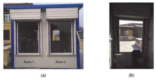
Figure 1.
External experimental house diagram (a) and internal room diagram (b).

Table 1.
Building’s enclosure parameters.
(2) Experimental Window
The ESIW system studied in this work was a house outfitted with special equipment, primarily comprised of a thermal insulation roller curtain, thermal insulation roller curtain box, and roller curtain rails. The core component of the thermal insulation roller curtain was a polyurethane thermal insulation board, which consisted of an aluminum alloy shell filled with 0.02 or 0.03 m of polyurethane. Figure 2 depicts the first generation of ESIW prototypes, which were installed at the outer window section of the ESIW system. Parameters of each ESIW structure are shown in Table 2.
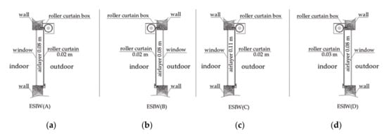
Figure 2.
Structure of the energy-saving insulation window (ESIW). Notes: (a) ESIW(A), (b) ESIW(B), (c) ESIW(C), and (d) ESIW(D).
Table 2.
Four window model structures.
The ESIW system could be rolled down to decrease heat loss on winter nights, rolled up to increase heat dissipation on summer nights, and left up at other times to ensure normal use and sunlight incidence through the glass window.
(3) Experimental Scheme
The left room in the experimental platform was named Room 1 and the right one was named Room 2. The four types of ESIW systems listed in Table 2 were respectively installed. In Room 1, ESIW(A) was installed outside the glass window, whereas ESIW(B) was installed inside the glass window. In Room 2, ESIW(C) was installed outside the glass window, and ESIW(D) was installed inside the glass window. Which structure was in use was determined by raising or lowering the thermal insulation roller curtain.
Pt100 resistance thermometers were used for taking temperature measurements. The recorded data represent the average temperatures of the measuring points. The temperature measurement accuracy was ± 0.1 °C. In order to obtain accurate temperature results, 64 Pt100 resistance thermometers and two THTZ temperature inspection instruments (Yuyao Tenghui temperature control instrument factory, Ningbo City, China) were adopted in two rooms to collect data for instant observation and recording. All the measurements were immediately saved on a memory card and displayed graphically on a computer screen to enable analysis of the test results. The air test points are shown in Figure 3, and the sizes shown in the figures reflect the locations of the resistance thermometers.
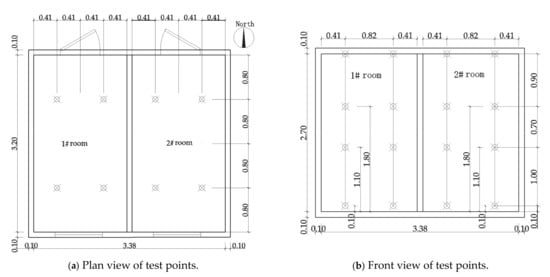
Figure 3.
Location of resistance thermometers.
The temperature of the air test points in Rooms 1 and 2 were measured from 1 to 4 January 2018. The measurement schedule and specifications are depicted in Table 3. Using this data, the house’s indoor average temperature was calculated for each of the four ESIW structures and then compared with the simulation results.
Table 3.
Measurement schedule and specifications.
2.2. Simulation Model
2.2.1. Airpak Model Setup
In order to build the Airpak model, following verification, Airpak software (Fluent Inc. New York, NY, USA) was used to generate a series of numerical simulations for the purpose of investigating the insulation performance of the four ESIW models (A, B, C, and D) under different influencing factors.
Airpak is a professional artificial environment system analysis software tool that was developed based on the FLUENT(CFD) technology software package. (Fluent Inc. New York, NY, USA) It is commonly used in the heating, ventilation, and air conditioning (HVAC) field, as it can accurately simulate physical phenomena such as air flow, heat transfer, and pollution in the study object [33].
(1) House Model
A 3.4 m × 1.84 m × 3 m (length × width × height) single room house model with a 0.97 m × 2 m (width × height) door was designed with Airpak software (Figure 4). In order to comprehensively analyze the temperature field within the room under different installation conditions, the following parameters were considered and are shown in Table 1: window thickness, window structure, and thermal parameters.
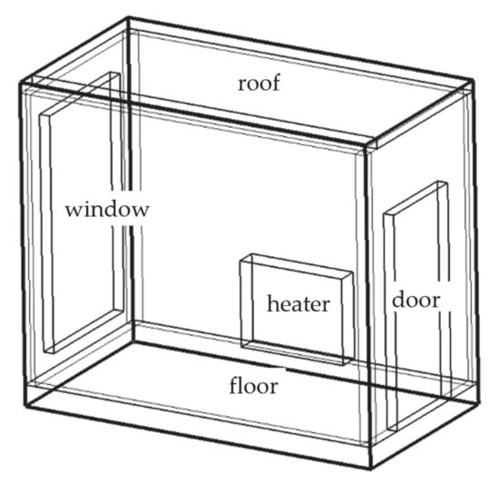
Figure 4.
Oblique axonometric view of the physical model.
(2) Window Model
The ESIW-structure window model exhibited dimensions of 1.2 m × 1.5 m (width × height), yet the thickness varied among the four tested varieties (Figure 5). In order to comprehensively analyze the temperature field of the air layer between the glass and the roller curtain, the following parameters were considered and are shown in Table 2: air layer thickness, window structure, and thermal parameters.
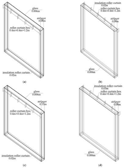
Figure 5.
Physical models (oblique axonometric view) of the four types of windows. Notes: (a) ESIW(A), (b) ESIW(B), (c) ESIW(C), and (d) ESIW(D).
(3) Simulation Mathematical Model
The simulation mathematical model used in this study was operated under the following conditions:
Air flow conforming to the Boussinesq hypothesis consisted of incompressible flow and steady turbulence.
Heat dissipation caused by a viscous force, and heat storage from the chimney wall, were ignored.
Air leakage was negligible in this model.
Outdoor environmental parameters, such as outdoor temperature and solar radiation, were constants.
The governing equations are depicted below according to the assumptions in [34].
Momentum equation:
Energy conservation equation:
where is the density vector, is the velocity vector, is static pressure, is the stress tensor, is gravitational acceleration, is other source terms that may arise from resistances or sources, etc., is the sensible enthalpy, is the source term that includes any defined volumetric heat sources, is the molecular conductivity, and is the conductivity due to turbulent transport.
(4) Grid Independence Test
A grid independence test was performed in order to ensure that the analysis results were not affected by the number of grid variations in the finite element analysis process.
The number of grids for A–G, as well as the simulation results, are shown in Table 4.
Table 4.
Results of the grid independence verification.
(5) Solver Setup
The two-equation model was adopted to simulate a turbulence effect in the simulation. To ensure computational accuracy, the discretization schemes for all the variables were second-order upwind schemes. A double algorithm was applied to couple pressure and velocity. The Discrete Ordinates (DO) radiation model was used to calculate the radiant heat transfer between different surfaces. The conservation of mass, momentum, and energy was governed by the Navier–Stokes equations, which were solved using the finite-volume method. The residuals were set at 10−4 for the continuity and momentum equations and 10−7 for the energy equation.
The parameters of the discretization solution are shown in Table 5.
Table 5.
The parameters of the discretization solution.
2.2.2. DeST Model Setup
DeST is a building energy consumption simulation software (Institute of environment and equipment, Tsinghua University, Beijing, China). The software platform applies computer simulation technology and unique simulation ideas to simulations of building environments, as well as that of air conditioning and refrigeration systems. The software simulations aid in making the architectural and HVAC system design more scientific and feasible, which is conducive to optimizing building and system performance. DeST software has a visual interface, which can realize staged design simulation and full condition simulation analysis [35].
After verification, DeST was used to compare energy consumption properties of a house with an ESIW structure window to that with six other window structures currently on the market. Thus, the DeST house model and several windows were built.
As shown in Figure 4, an identical house model was also established using DeST building energy simulation software. All the building structures and parameters were similar to those of the experimental house built in the laboratory.
The house’s room function was simplified and treated as a heated living room. The upper and lower limits of the indoor design temperature were 26 °C and 18 °C, respectively. There was no person, lighting, or other heating equipment in the room. Taiyuan City meteorological parameters were adopted and obtained from the hourly meteorological data generation software Medpha (Institute of environment and equipment, Tsinghua University, Beijing, China).
3. Results and Discussion
3.1. Model Validation
(1) DeST Model Validation
In order to analyze the effectiveness of the DeST software, a comparative analysis was conducted between the experimental and simulated data (Figure 6).
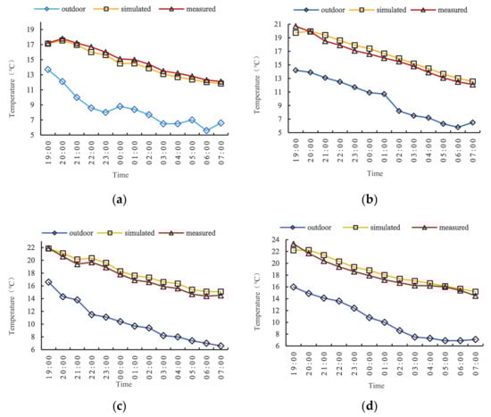
Figure 6.
Comparison between simulated and measured temperature. Notes: (a–d) represent a room with insulated ESIW window structures (A, B, C, and D) respectively.
Figure 6 demonstrates that the measured temperature trend and model temperature trend were reasonably consistent. When the absolute value of the relative average deviation was <15% and the root mean square error was <35%, the simulation results were considered to be within the acceptable error range and therefore reliable. The average deviation between the simulated value and the measured value for structures A, B, C, and D were 2.71%, 3.08%, 3.63%, and 3.07%, respectively, which were all far below 15%. Furthermore, the root mean square errors were 3.05%, 4.15%, 4.02%, and 4.18%, respectively, and were therefore significantly less than 35%. As such, the DeST model adopted for this work can be used to accurately simulate the natural room temperature of energy-saving insulated windows with various structures.
(2) Airpak Model Validation
Results from measurements in the experimental room were used to validate the computational model. The numerical validation procedures were designed to fully replicate the experimental work. Figure 7 shows the comparisons between the measured and simulated air temperature at three different vertical positions within the test chamber. The agreement between the measured and modeled temperature profiles in the experimental room were within the acceptable error range.
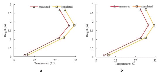
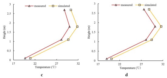
Figure 7.
Comparison of simulated and measured temperature profiles. Room with (a) ESIW(A), (b) ESIW(B), (c) ESIW(C), and (d) ESIW(D).
3.2. Comparison of Different Energy-Saving Windows
In order to comprehensively analyze the advantages of the ESIW structure relative to other thermal insulation windows, the natural room temperature, the cooling and heating load on the hottest and coldest days of the year, the total annual cooling and heating load, and the price–load ratio (PLR) for houses with seven different window types were compared and analyzed using the simulation tool. The parameters of the seven window types are shown in Table 6. For comparison purposes, the 6 mm glass window (#2) was considered the base case. Note that ESIW(A) was selected to represent all four types of ESIW windows.
Table 6.
Performance parameters of different energy-saving thermal insulation windows.
(1) Comparison at Natural Room Temperature
The natural hourly room temperature on 5 January (Figure 8) and 31 July (Figure 9), the coldest and hottest days of the year, respectively, was compared between the seven houses with different window structures.
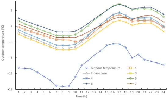
Figure 8.
Room temperature for seven houses with different energy-saving windows.
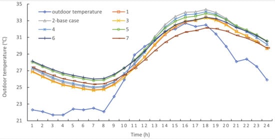
Figure 9.
Room temperature for seven houses with different energy-saving windows.
Figure 8 and Figure 9 show that on the coldest day of the year, the lowest temperature of the room with an ordinary glass window (#2) was −5.43 °C, whereas that of the room with the ESIW(A) window (#1) was −2.31 °C. Due to the night heat insulation effect induced by the thermal insulation curtain, the natural indoor temperature of houses with ESIW(A) windows was generally higher than that of houses with ordinary 6 mm glass windows (#2). This phenomenon was particularly apparent at night. For rooms with single-layer functional glass windows (#3 and #4), the minimum temperature was between −4 °C and −5.5 °C, which was not significantly higher than that of the room with ordinary glass (#2). The temperature of the rooms with double- (#5) or triple- (#7) layered glass windows and argon-filled low-radiation glass windows (#6) was significantly improved, with the lowest temperatures ranging between −0.98 °C and 0.22 °C.
On the hottest day of the year, due to the external shading structure, the maximum temperature of the room with the ordinary glass window (#2) was 34.5 °C, whereas that of the room with the ESIW(A) window (#1) was 33.1 °C. Houses with ESIW(A) windows generally exhibited a lower natural indoor temperature than houses with ordinary 6 mm glass windows (#2). This was particularly apparent in the afternoon. For the single-layer functional glass windows (#3 and #4), the maximum temperature ranged between 33 °C and 34 °C and did not decrease significantly compared with those composed of ordinary 6 mm glass (#2). At ~32.3 °C, the temperature of the rooms with double- (#5) or triple- (#7) layered glass windows and argon-filled low-radiation glass windows (#6) was significantly lower, demonstrating an evident, relative reduction in temperature.
(2) Indoor Load Comparison
The hourly heating load and cooling load on 5 January and 31 July, the coldest and hottest days of the year, respectively, is shown in Figure 10 and Figure 11, respectively.
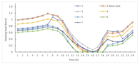
Figure 10.
Heating load for houses with different energy-saving windows on the coldest day of the year.
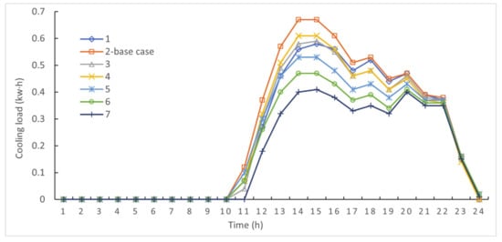
Figure 11.
Cooling load for houses with different energy-saving windows on the hottest day of the year.
As shown in Figure 10, on the coldest day of the year, the maximum heating load of the room with ordinary 6 mm glass (#2-base case) was 1.19 kW × h, and the 24 h cumulative heating load was 16.18 kW × h. By comparison, the maximum heating load of houses with ESIW(A) windows (#1) was 1.08 kW × h, and the cumulative heating load was 13.89 kW × h. Due to the night heat insulation effect induced by the thermal insulation curtain, the indoor heating load of houses with ESIW(A) windows (#1) was generally lower than that of houses with ordinary 6 mm glass windows (#2). This is particularly apparent at night. For the single-layer functional glass windows (#3 and 4), the maximum heating load was 1.18 kW × h and the cumulative heating load was 14–17 kW × h. Thus, the maximum heating load of houses with single-layer functional glass windows (#3 and 4) did not significantly decrease when compared with that comprised of ordinary 6 mm glass windows (#2). The maximum heating load of 0.75 kW × h, and cumulative heating load of 8-9 kW × h exhibited by double- (#5) and triple- (#7) layered glass windows and argon-filled low-radiation glass windows (#6) shows that they can significantly reduce the heating load.
On the hottest day of the year (Figure 11), the maximum cooling load of the room with ordinary 6 mm glass (#2-base case) was 0.67 kW × h, and the cumulative cooling load was 5.90 kW × h. By comparison, the maximum cooling load of houses with ESIW(A) windows (#1) was 0.58 kW × h, and the cumulative cooling load was 5.33 kW × h. The indoor cooling load of houses with ESIW(A) structural windows (#1) was generally lower than that of houses with ordinary 6 mm glass windows (#2). This was particularly apparent in the afternoon. For the rooms comprised of single-layer functional glass windows (#3 and 4), the maximum cooling load was 0.60 kW × h, and the cumulative cooling load was 4.97–5.35 kW × h. Thus, the maximum cooling load of houses with single-layer functional glass windows (#3 and 4) did not significantly decrease when compared to those comprised of ordinary 6 mm glass windows (#2). The maximum cooling load of 0.45 kW × h, and the cumulative cooling load of 3.95–4.51 kW × h exhibited by double- (#5) and triple- (#7) layered glass windows and argon-filled low-radiation glass windows (#6) shows that they can significantly reduce the cooling load.
(3) Comprehensive Performance Comparison
Using the data obtained from steps 1 and 2 above, the cumulative annual load and the price–load ratio (PLR) were calculated and compared. The house’s total annual load was calculated for windows #1 and #3–7, respectively, and divided by that of the house outfitted with 6 mm transparent glass windows (#2). The quotient is referred to as the “load difference.” Next, the PLR was calculated by dividing the price of windows #1 and #3–7 with their load differences (Table 7 and Figure 12).
Table 7.
Price and energy parameters of different energy-saving thermal insulation windows.
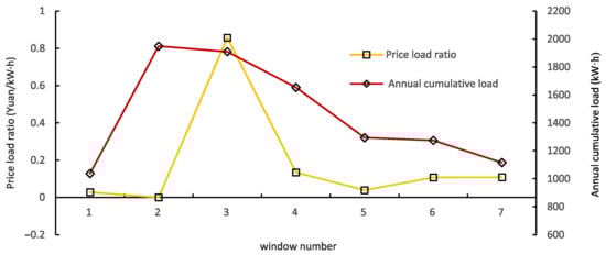
Figure 12.
The annual cumulative load and the price per relative load for each energy-saving window type.
Figure 12 shows that the cumulative annual load of a room with an ordinary glass window (#2) was 1948.71kW × h. Due to the night insulation effect induced by the thermal insulation curtain, houses with ESIW(A) structure windows (#1) exhibited a cumulative annual load of 1370.21 kW × h, which was generally lower than houses with ordinary 6 mm glass windows (#2). For rooms with single-layer functional glass windows (#3 and 4), the cumulative annual load was 1653–1908 kW × h; thus, the thermal load was not significantly reduced compared to rooms composed of ordinary glass (#2). The temperature of the rooms with double- (#5) and triple- (#7) layered glass windows and argon-filled low-radiation glass windows (#6) significantly reduced the cumulative annual load, which ranged from 1120–1290 kW × h.
Using the cost and energy consumption analysis results of each window type, a comprehensive index of the PLR (Yuan/kW × h) was developed. The lower the value, the more superior the window performance. Figure 12 demonstrates that houses with ESIW(A) structural windows (#1) had a PLR equal to 0.028 Yuan/kW × h. For rooms with single-layer functional glass windows (#3 and #4), the PLR was 0.13–0.86 Yuan/kW × h, a reflection of the material’s high cost. Rooms with double- (#5) and triple- (#7) layered glass windows and argon-filled low-radiation glass windows (#6) had better energy consumption performance, but were also expensive. Thus, the PLR of these windows ranged from 0.039–0.108 Yuan/kW × h. Table 7 also demonstrates that the ESIW window could achieve a carbon dioxide emission reduction of 4.61 kg/(m2 × year). Thus, the environmental benefits are significant.
(4) Summary for the Comparison Analysis
Compared to houses with ordinary 6 mm glass windows, houses outfitted with the ESIW(A) window generally showed improved natural indoor temperature, as the heating load, cooling load, and cumulative annual load all clearly decreased. Houses with windows made from single-layer functional glass (two types were tested) showed no obvious temperature improvement and no discernable decrease in the load value. For the two- and three-layered glass windows and the argon-filled glass window, the temperature showed relatively obvious improvement; thus, the load value decreased in response.
The price–load ratio of ESIW(A) windows was 0.028 Yuan/kW × h, whereas that of the two single-layer functional glass windows ranged from 0.13–0.86 Yuan/kW × h. The two- and three-layered glass windows and argon-filled glass windows demonstrated superior energy consumption performance, but at a significantly higher cost, with a price–load ratio of 0.039–0.108 Yuan/kW × h.
In conclusion, among the seven tested structures, ESIW(A) showed superior temperature distribution and the lowest cost performance.
3.3. Single Factor Simulation
In order to comprehensively analyze the room’s temperature field response to different ESIW system windows, the following simulations were conducted using the single-factor simulation method. An outdoor temperature of −12 °C was selected in order to mimic winter nighttime conditions. Table 8 lists some critical factors that were strongly correlated with the model house’s average temperature. Among them are WWR—the ratio of the area of windows in a certain direction to the total area of the enclosure structure in that direction, HTC—the four kinds of energy-saving windows and ordinary windows described in this paper, and ESS—the actual materials comprising the different enclosure structures. Table 9 displays the heat transfer coefficient of some enclosures with different ESSs.
Table 8.
Numerical analysis factors and levels.
Table 9.
Heat transfer coefficient of some enclosures with different energy-saving standards. [W/m2 × K].
WWR, electric heater power, HTC, and ESS were the four factors selected for analysis. Using the same outdoor temperature, room temperature measurements were obtained under the following combinations: Figure 13a—5 HTCs with 5 WWRs, Figure 13b—5 HTCs with 3 ESSs, Figure 13c—5 WWRs with 3 ESSs (HTC = 1.02 W/m2 × °C, power = 1000 W), Figure 13d—5 WWRs with 3 ESSs (HTC = 5.11 W/m2 × °C, power = 1000 W), Figure 13e—3 ESSs with 5 WWRs (HTC = 1.02 W/m2 × K, power = 1000 W), and Figure 13f—3 ESSs with 5 WWRs (HTC = 5.11 W/m2 × K, power = 1000 W), totaling 75 individual experiments. The five test values for HTC, WWR, and heater power, as well as three test values for ESS, are depicted in Table 7.
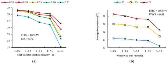
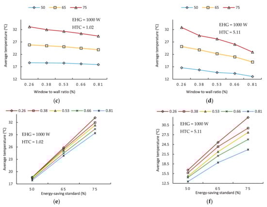
Figure 13.
Variations in average temperature in response to changing factors.
Figure 13a shows changes in the average temperature as a function of varying HTCs and WWRs. Note that the temperature decreased as a function of increasing HTC, but the degree of change enlarged as the HTC increased. Furthermore, the smaller the WWR at a given HTC, the higher the temperature. Thus, when the HTC was small enough, enlarging the WWR was not problematic. As such, building envelope HTC limitations in some building standards can be modified to meet the various demands of people in the building.
Figure 13b shows changes in average temperature as a function of varying HTCs and ESSs. Note that for each HTC, the average temperature gradually increased as the ESS increased, because less heat was lost due to the presence of more building envelope insulation.
Figure 13c,d shows changes in average temperature as a function of varying WWRs and ESSs. Note that when HTC was 5.11, the temperature dropped faster compared to when it was 1.02, because of the smaller thermal resistance.
Figure 13e,f shows that as the ESS and corresponding building envelope insulation increased, the average temperature increased in parallel. Furthermore, the higher the ESS and HTC, the higher the temperature difference among different WWRs. Thus, as the ESS increases, the WWR and HTC become progressively more critical.
3.4. Other Temperature Indexes
To get a more comprehensive understanding of how average temperature is impacted by HTC and WWR, three other indexes—average 1.1 m, door, and window temperatures—were measured and the results were compared to the average temperature trend obtained from the previous experiment.
Figure 14a,b show that all three indexes depicted a temperature decrease as a function of increasing HTC and WWR. Essentially, as the amount of heat loss increased, the average temperature and that of the other three indexes all jointly decreased. Across all four HTCs, the 1.1 m average temperature remained the highest and was followed by the overall average temperature, which was higher than both the average window and door temperatures. As long as the HTC was <1.71, the average door temperature was less than that of the window. However, when the HTC increased to 5.11, the average window temperature dropped below that of the door, because more heat loss occurred through the less insulated window.
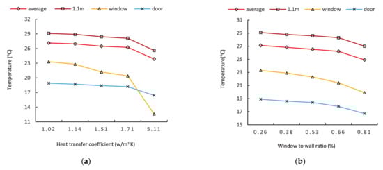
Figure 14.
Variations of the temperature indexes as a function of the increasing (a) heat transfer coefficient (HTC) and (b) window-to-wall ratio (WWR).
3.5. ESIW Heat Transfer Coefficient
Calculating the ESIW HTC under different conditions required us to build a group of formulas. After several complex simulations, the HTC and air infiltration flow (Qair) in the air layer were obtained for four different ESIW structures under different outdoor air speeds. The results are shown in Figure 15 and Figure 16, respectively.
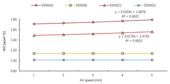
Figure 15.
HTC distribution of different ESIW structures at different air speeds.
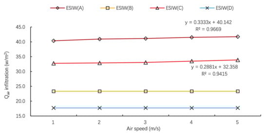
Figure 16.
Qair infiltration of different ESIW structures at different air speeds.
As shown in Figure 15 and Figure 16, ESIW(A) and ESIW(C), which had the roller curtain installed outside the glass, exhibited remarkably different results compared with ESIW(B) and ESIW(D), which had the roller curtains installed inside the glass.
For the ESIW(A) and ESIW(C) systems, both the HTC and Qair infiltration increased as a function of air speed. Essentially, a faster airspeed correlated with more heat loss during the airflow process in the air layer between the glass and the roller curtain. As more heat was transferred out of the air layer, the HTC increased. For the ESIW(B) and ESIW(D) systems, both the HTC and Qair infiltration remained stable, despite the increasing air speed. Thus, there was no additional heat loss from the air flow process in the air layer between the glass and roller curtain. Due to the roller curtain being installed inside the glass, the air flow occurred in the indoor environment; thus, no convective heat transfer transpired.
In addition, the results also demonstrate the differences between the four windows’ energy-saving and insulation characteristics. ESIW(D) had the best performance due to the lower HTC and Qair infiltration, whereas ESIW(A) had the poorest performance due to the higher HTC and Qair infiltration. Because the windows with the roller curtains installed inside the glass had no air infiltration, they were clearly superior to those with outer installation.
In summary, at any given fixed speed, the window’s HTC and Qair infiltration trend was as follows: ESIW(A) > ESIW(C) > ESIW(B) > ESIW(D).
For further analysis, the following formulas can be used to predict the HTC or Qair infiltration under different conditions:
For the ESIW(A) system,
For the ESIW(C) system,
where y is the system’s HTC and x is the air flow speed. If the air speed can be obtained, the HTC can be easily calculated.
For ESIW(A) system,
For ESIW(C) system,
where y is the system’s Qair infiltration and x is the air flow speed. If the air speed can be obtained, the Qair infiltration can be easily calculated.
3.6. Response Surface Analysis
Response surface analysis was performed in order to determine the appropriate weight of the key factors, as well as the relationship between them. Three factors and three levels were considered, as shown in Table 10. All 27 experiments were performed in triplicate and in random order. The experimental data are presented in Table 11.
Table 10.
Three factors on three levels in response to surface analysis.
Table 11.
Design arrangement and responses in terms of thermal efficiency index η.
The equations used to calculate the thermal efficiency index η include:
where is the average temperature of the model room after a simulation, is the temperature of the model environment (−12 °C), and is the electric heater power in the model house, in this case set to 1000 W in order to make the results clear.
A multiple regression equation was used to fit the second-order polynomial equation shown in Formula (9):
where Y is the predicted response for the thermal efficiency index η; β0 is the fitted response value at the central point of the design; β1, β2, and β3 are linear terms; β12, β13, and β23 represent interaction effects; and β11, β22, and β33 are squared effects.
Statistical analysis was performed using the software Stat-Ease Design-Expert 8.0.6.1 Trial computer program (Stat-Ease Inc., Minneapolis, MN, USA). Analysis of variance (ANOVA) and Tukey tests were used to verify the statistical significance with a confidence level of 95.0%. ANOVA produced parameters for lack of fit, coefficient of determination, and F-tests, which were employed to evaluate the model adequacy [36]. The model was fitted by multiple linear regressions and the obtained response surface plots are depicted in Table 12 and Figure 17.
Table 12.
Coefficients and analysis of variance for the fitted models.
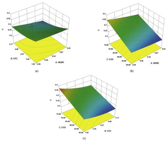
Figure 17.
The effect of WWR, HTC, and ESS on the thermal efficiency index η: (a) HTC and WWR, (b) ESS and WWR, and (c) ESS and HTC.
The results from this study show that the thermal efficiency was affected by HTC and WWR, ESS and WWR, and HTC and WWR.
HTC and WWR had a negative and significant linear effect (p < 0.05), and the interaction between these two variables was also negative and significant (p < 0.05). Figure 17a shows that thermal efficiency significantly decreased with increasing HTC and WWR. These results may be attributed to increased thermal loss ability at a higher HTC and increased thermal loss area at higher WWR.
In addition, ESS and WWR showed a significant linear effect (p < 0.05), and the interaction between these two variables was positive and significant (p < 0.05). Figure 17b shows that the thermal efficiency significantly decreased with increasing HTC and significantly increased with increasing ESS. These results may be attributed to increased thermal loss ability at a higher HTC and better house envelope insulation at a higher ESS.
Finally, HTC and WWR exhibited a significant linear effect (p < 0.05), and the interaction between these two variables was positive and significant (p < 0.05). Figure 17c shows that the thermal efficiency significantly decreased with increasing WWR and significantly increased with increasing ESS. These results could be attributed to increased thermal loss area at a higher WWR and better house envelope insulation at a higher ESS.
The regression model equation enabled the effects of the three variables on the response to be predicted, and Response surface methodology (RSM) was performed to optimize the three variables. The predicted responses are presented in Table 13. For convenience, the optimal conditions were set as follows: HTC = 1.07 W/m2 × K, WWR = 0.26, and ESS = 75%. The experimental values were in good agreement with the predicted values, so the conditions obtained by RSM were accurate, reliable, and practical.
Table 13.
Predicted and experimental values of response at optimum conditions.
4. Conclusions
A series of numerical simulations was carried out to investigate the insulation performances of the ESIW system under different influencing factors. The major findings are summarized as follows:
- (1)
- The ESIW(A) structure window exhibited a more suitable indoor natural temperature; less heating load, cooling load, and cumulative annual load; and a more feasible price–load ratio than other energy-saving windows. Thus, the ESIW-structure windows are suitable for building insulation.
- (2)
- Single factor analysis of the ESIW structures showed that the average indoor temperature gradually decreases as a function of increasing HTC and WWR, and increases in response to increasing electric heater power and ESS.
- (3)
- The degree of temperature decline among different WWRs changes as a function of the HTC; the smaller the HTC, the smaller the temperature decline. Thus, when the HTC is small enough, enlarging the WWR should not create any problems. In addition, as the ESS increases, the average temperature change and HTC or WWR jointly increase. Thus, as the ESS increases, the WWR and HTC become progressively more critical.
- (4)
- After executing several complex simulations, the HTC and Qair in the air layer were obtained for four different ESIW windows under different outdoor air speeds. If the air speed can be obtained, the HTC and Qair infiltration can be easily calculated.
- (5)
- RSM results showed that thermal efficiency was significantly affected by HTC, WWR, and ESS. The interactions between HTC and WWR, HTC and ESS, and WWR and ESS were negative, positive, and positive, respectively. The optimal thermal efficiency conditions consisted of HTC = 1.02 W/m2 × K, WWR = 0.26, and ESS = 75%.
Rolling down the curtain resulted in less heat loss during winter nights, and pulling up the curtain enabled normal daylight absorption during all other times of the year. The ESIW structure insulation window can significantly reduce the annual load of the building, with minimal input cost. In future follow-up research, more flexible insulation material with optimal functional properties and thermal stability should be used, and additional and varied types of building facades, such as curtain- walls, should be investigated in order to determine the ideal combination for use in building insulation. Although the control system was not the focus of this study, in practical application, it can be realized by adding a timing control system to activate and deactivate the motor. Finally, condensation should be considered in the process of popularizing ESIW windows in areas with humidity issues.
5. Patents
An invention patent named “A utility model relates to a solar energy collecting, shading, energy saving and heat preservation window” was granted by the national intellectual property administration of China in 2018. The patent number is ZL 201610854569.3, and the inventors were Qi Tian and Zhiqiang Wang.
Author Contributions
Conceptualization, Z.W. and Q.T.; data curation, J.J.; formal analysis, Z.W.; funding acquisition, Q.T.; investigation, Z.W.; methodology, Z.W.; project administration, Q.T.; resources, Q.T.; software, J.J.; supervision, Q.T.; validation, Z.W.; visualization, J.J.; writing—original draft, Z.W.; writing—review and editing, J.J. and Q.T. All authors have read and agreed to the published version of the manuscript.
Funding
This research was funded by the National 12th Five-Year Science and Technology Support Plan (grant No.2012BAJ04B02) from the National Natural Science Foundation of China (NSFC), and the International Cooperation Project (grant No.2013DFA61580) from the Ministry of Science and Technology of China (MOST), and the National Natural Science Foundation of China (grant No. 51808372) and Key Research and Development (R&D) Projects of Shanxi Province (grant No. 201903D121037), and the Application Foundation Research Plan of Shanxi Province (grant No. 201801D221348), and the Scientific and Technological Innovation Programs of Higher Education Institutions in Shanxi (grant No. 201802046), and the China Postdoctoral Science Foundation (grant No. 2017M611200).
Institutional Review Board Statement
Not applicable.
Informed Consent Statement
Not applicable.
Data Availability Statement
Data is contained within the article.
Acknowledgments
We gratefully acknowledge the help of Xu Dong, Bin Wu and Lin Li for the supporting of the on-site experiments.
Conflicts of Interest
The authors declare no conflict of interest.
Nomenclature
| English Symbols | |
| TS | Solar transmittance (%) |
| TV | Visible light transmittance (%) |
| RS | Solar reflectivity (%) |
| RV | Visible light reflection rate (%) |
| U | Overall heat transfer coefficient (W/m2 × K) |
| Qair | Flow of air infiltration (m3/s) |
| w | Work done by the heater (W) |
| g | Acceleration of gravity (m/s2) |
| T | Temperature |
| Greek Symbols | |
| Thickness (mm) | |
| Density (kg/m3) | |
| Thermal conductivity (W/m × K) | |
| Thermal efficiency index (°C/W) | |
| Velocity vector (m/s) | |
| Abbreviations | |
| ALT | Air layer thickness between the roller curtain and the glass |
| ESIW | Energy-saving insulated window |
| TEM | Thickness of embedded material in the roller curtain |
| OW | Ordinary 6 mm glass window |
| RSM | Response surface methodology |
| HTC | Heat transfer coefficient |
| PV | Photovoltaic window |
| HSW | Heat storage walls |
| TIM | Transparent insulation material |
| PCM | Phase-changing materials |
| WWR | Window-to-wall ratio |
| ESS | Energy-saving standard of building |
| SHGC | Solar heat gain coefficient |
| SC | Shading coefficient |
| PVC | Polyvinyl chloride |
References
- Xu, X.L.; Feng, G.H.; Chi, D.D.; Liu, M.; Dou, B.Y. Optimization of Performance Parameter Design and Energy Use Prediction for Nearly Zero Energy Buildings. Energies 2018, 11, 3252. [Google Scholar] [CrossRef]
- Talberga, R.; Jelle, B.P.; Loonen, R.; Gao, T.; Hamdy, M. Comparison of the energy saving potential of adaptive and controllable smart windows: A state-of-the-art review and simulation studies of thermochromic, photochromic and electrochromic technologies. Sol. Energy Mater. Sol. Cells 2019, 200, 109828. [Google Scholar] [CrossRef]
- Zhong, K.C.; Li, S.H.; Sun, G.F.; Li, S.S.; Zhang, S.S. Simulation study on dynamic heat transfer performance of PCM-filled glass window with different thermophysical parameters of phase change material. Energy Build. 2015, 106, 87–95. [Google Scholar] [CrossRef]
- Berardi, U. The development of a monolithic aerogel glazed window for an energy retrofitting project. Appl. Energy 2015, 154, 603–615. [Google Scholar] [CrossRef]
- Sun, L.L.; Hu, W.J.; Yuan, Y.P.; Gao, X.L.; Lei, B. Dynamic Performance of the Shading-Type Building-Integrated Photovoltaic Claddings. Procedia Eng. 2015, 121, 930–937. [Google Scholar] [CrossRef]
- Cuce, E.; Young, C.H.; Riffat, S.B. Thermal performance investigation of heat insulation solar glass: A comparative experimental study. Energy Build. 2015, 86, 595–600. [Google Scholar] [CrossRef]
- Gao, T.; Jelle, B.P.; Ihara, T.; Gustavsen, A. Insulating glazing units with silica aerogel granules: The impact of particle size. Appl. Energy 2014, 128, 27–34. [Google Scholar] [CrossRef]
- Cha, J.H.; Kim, S.H.; Park, K.W.; Lee, D.R.; Jo, J.H.; Kim, S. Improvement of window thermal performance using aerogel insulation film for building energy saving. J. Therm. Anal. Calorim. 2014, 116, 219–224. [Google Scholar] [CrossRef]
- Alfano, F.R.A.; Isola, M.D.; Ficco, G.; Palella, B.I.; Riccio, G. Experimental Air-Tightness Analysis in Mediterranean Buildings after windows retrofit. Sustainability 2016, 8, 991. [Google Scholar] [CrossRef]
- Yoo, S.H.; Jeong, H.K.; Ahn, B.L.; Han, H.; Seo, D.H.; Lee, J.H.; Jang, C.Y. Thermal transmittance of window systems and effects on building heating energy use and energy efficiency ratings in South Korea. Energy Build. 2013, 67, 236–244. [Google Scholar] [CrossRef]
- Lee, E.S.; Pang, X.F.; Hoffmann, S.; Goudey, H.; Thanachareonkit, A. An empirical study of a full-scale polymer thermochromic window and its implications on material science development objectives. Sol. Energy Mater. Sol. Cells 2013, 116, 14–26. [Google Scholar] [CrossRef]
- Ye, H.; Meng, X.C.; Long, L.S.; Xu, B. The route to a perfect window. Renew. Energy 2013, 55, 448–455. [Google Scholar] [CrossRef]
- An, H.J.; Yoon, J.H.; An, Y.S.; Heo, E. Heating and cooling performance of office buildings with a-si bipv windows considering operating conditions in temperate climates: The case of Korea. Sustainability 2018, 10, 4856. [Google Scholar] [CrossRef]
- Buratti, C.; Moretti, E. Glazing systems with silica aerogel for energy savings in buildings. Appl. Energy 2012, 98, 396–403. [Google Scholar] [CrossRef]
- Gasparella, A.; Pernigotto, G.; Cappelletti, F.; Romagnoni, P.; Baggio, P. Analysis and modelling of window and glazing systems energy performance for a well insulated residential building. Energy Build. 2011, 43, 1030–1037. [Google Scholar] [CrossRef]
- Amirkhani, S.; Jahromi, A.B.; Mylona, A.; Godfrey, P.; Cook, D. Impact of low-e window films on energy consumption and co2 emissions of an existing UK hotel building. Sustainability 2019, 11, 4265. [Google Scholar] [CrossRef]
- Baek, S.H.; Kim, S.C. Optimum Design and Energy Performance of Hybrid Triple Glazing System with Vacuum and Carbon Dioxide Filled Gap. Sustainability 2019, 11, 5543. [Google Scholar] [CrossRef]
- Lu, Y.; Lin, H.K.; Liu, S.W.; Xiao, Y.Q. Nonuniform woven solar shading screens: Shading, mechanical, and daylighting performance. Sustainability 2019, 11, 5652. [Google Scholar] [CrossRef]
- Hatamipour, M.S.; Mahiyar, H.; Taheri, M. Evaluation of existing cooling systems for reducing cooling power consumption. Energy Build. 2007, 39, 105–112. [Google Scholar] [CrossRef]
- Wang, J.H.; Zhang, T.F.; Wang, S.G.; Battaglia, F. Numerical investigation of single-sided natural ventilation driven by buoyancy and wind through variable window configurations. Energy Build. 2018, 168, 147–164. [Google Scholar] [CrossRef]
- Yun, G.Y. Influences of perceived control on thermal comfort and energy use in buildings. Energy Build. 2018, 158, 822–830. [Google Scholar] [CrossRef]
- Sun, Y.Y.; Liang, R.Q.; Wu, Y.P.; Wilson, R.; Rutherford, P. Glazing systems with parallel slats transparent insulation material(ps-tim): Evaluation of building energy and daylight performance. Energy Build. 2018, 159, 213–227. [Google Scholar] [CrossRef]
- Pan, S.; Xiong, Y.Z.; Han, Y.Y.; Zhang, X.X.; Xia, L.; Wei, S.; Wu, J.S.; Han, M.J. A study on influential factors of occupant window-opening behavior in an office building in China. Build. Environ. 2018, 133, 41–50. [Google Scholar] [CrossRef]
- Leivo, V.; Prasauskas, T.; Du, L.L.; Turunen, M.; Kiviste, M.; Aaltonen, A.; Martuzevicius, D.; Shaughnessy, U.H. Indoor thermal environment, air exchange rates, and carbon dioxide concentrations before and after energy retro fits in Finnish and Lithuanian multi-family buildings. Sci. Total Environ. 2018, 621, 398–406. [Google Scholar] [CrossRef] [PubMed]
- Souayfane, F.; Biwole, P.H.; Fardoun, F. Thermal behavior of a translucent superinsulated latent heat energy storage wall in summertime. Appl. Energy. 2018, 217, 390–408. [Google Scholar] [CrossRef]
- Chen, C.; Ling, H.S.; Zhai, Z.Q.; Li, Y.; Yang, F.G.; Han, F.T.; Wei, S. Thermal performance of an active-passive ventilation wall with phase change material in solar greenhouses. Appl. Energy. 2018, 216, 602–612. [Google Scholar] [CrossRef]
- Liu, Z.J.; Wu, D.; Yu, H.C.; Ma, W.S.; Jin, G.Y. Field measurement and numerical simulation of combined solar heating operation modes for domestic buildings based on the Qinghai–Tibetan plateau case. Energy Build. 2018, 167, 312–321. [Google Scholar] [CrossRef]
- Li, Y.R.; Zhou, J.; Long, E.S.; Meng, X. Experimental study on thermal performance improvement of building envelopes by integrating with phase change material in an intermittently heated room. Sustain. Cities Soc. 2018, 38, 607–615. [Google Scholar] [CrossRef]
- Ran, J.D.; Tang, M.F. Passive cooling of the green roofs combined with night-time ventilation and walls insulation in hot and humid regions. Sustain. Cities Soc. 2018, 38, 466–475. [Google Scholar] [CrossRef]
- Marani, A.; Madhkhan, M. An innovative apparatus for simulating daily temperature for investigating thermal performance of wallboards incorporating PCMs. Energy Build. 2018, 167, 1–7. [Google Scholar] [CrossRef]
- Guldentops, G.; Ardito, G.; Tao, M.J.; Focil, S.G.; Dessel, S.V. A numerical study of adaptive building enclosure systems using solid–solid phase change materials with variable transparency. Energy Build. 2018, 167, 240–252. [Google Scholar] [CrossRef]
- Zong, Y.; Li, D.; Teng, J.Y. Energy saving and economic analysis of window glass selection scheme for residential buildings in Wuhan. New Build. Mater. 2014, 1, 36–39. [Google Scholar]
- Tian, T.Y.; Wang, L.; Chang, J.Q. Numerical simulation of pollutant dissipation in large scale workshop based on Airpak. Saf. Environ. Eng. 2012, 12, 31–35. [Google Scholar]
- Mao, N.; Zhang, B.; Song, M.J.; Deng, S.M. A simplified numerical study on the energy performance and thermal environment of a bedroom TAC system. Energy Build. 2018, 166, 305–316. [Google Scholar] [CrossRef]
- Peng, G.Z.; Miao, X.P.; Hu, X. Simulating the influence of windows on energy consumption of air conditioning system by DeST. Clean. Air Cond. Technol. 2006, 3, 19–24. [Google Scholar]
- Pierucci, A.; Cannavale, A.; Martellotta, F.; Fiorito, F. Smart windows for carbon neutral buildings: A life cycle approach. Energy Build. 2018, 165, 160–171. [Google Scholar] [CrossRef]


Publisher’s Note: MDPI stays neutral with regard to jurisdictional claims in published maps and institutional affiliations. |
© 2021 by the authors. Licensee MDPI, Basel, Switzerland. This article is an open access article distributed under the terms and conditions of the Creative Commons Attribution (CC BY) license (http://creativecommons.org/licenses/by/4.0/).