Abstract
The growing interest in saving building energy has increasingly motivated studies on model predictive control (MPC), where system operation proceeds according to a planned operation strategy. Data-driven models that perform learning using past operation data of buildings are favorable for MPC applications owing to their fast computation speed. However, it is difficult to apply MPC to buildings with insufficient operation data, as the prediction accuracy varies depending on the data used for learning. To address this, we propose a method that involves generating data through a detailed building energy model and utilizing a long short-term memory (LSTM) network that performs learning using the data as an MPC model. The model was verified through a comparison with the reference model using the same optimization algorithm. In the MPC of the objective function, which is to reduce electrical energy expenditure by optimizing the indoor temperature of the target building, approximately 35% grid energy consumption was reduced compared to a reference case, by increasing self-consumption of photovoltaic (PV) energy and avoiding PV curtailment. Further, the required computation time was reduced to approximately 30%, even including the data generation time for daily learning, thereby confirming the feasibility of the MPC model that employs LSTM.
1. Introduction
A considerable proportion of building energy is used for heating, ventilating, and air conditioning (HVAC) operations. Hence, the energy consumption of a building can be reduced through the optimal control of its heat source and HVAC systems [1,2]. In particular, the number of studies on model predictive control (MPC), in which system operation is performed according to a strategy planned in advance through building and system models, has been continuously increasing to improve building energy saving and the efficient operation of facility systems. Studies performing simulations [3,4,5] and various empirical studies for actual buildings have been conducted [6,7,8]. According to previous studies, the MPC method demonstrated the possibility of saving 15–30% energy, depending on various factors related to the thermal performance and renewable energy of buildings. The Automatic Control Laboratory in Zurich, Switzerland, likewise reported energy saving at a similar level through the OptiControl project, in which large-scale MPC research was conducted for two years [9]. The application of MPC to building control has a large potential for energy saving. The most important element that determines the performance of MPC is the prediction accuracy of the building model [10,11,12]. Detailed energy analysis software programs, such as EnergyPlus, TRNSYS, and ESP-r, can be used for building modeling. According to Privara et al. [13], however, it is difficult to directly use these methods for control, because they involve complicated models, a long computation time, and non-explicit expressions of parameters in many cases. Hoes et al. [14] also mentioned that the use of advanced control algorithms has limitations, because detailed analysis programs do not allow external access to all parameters for control. Studies were also conducted to directly apply control algorithms to detailed analysis programs [15,16,17]; however, the simulation requires considerable computation time, as the data exchange with an external program must be performed through a virtual test bed, such as the building control virtual test bed. Hence, it is necessary to consider methods to supplement these shortcomings for MPC that must establish daily or real-time building operation strategies [18,19].
In recent years, studies on MPC have been actively conducted using data-driven models, which explain the dynamic behavior of a building through correlations among data. Data-driven models explain the thermal behavior of a building through input-output relationships in data, such as the operation data of the building and weather, unlike detailed analysis programs based on the physical equations of various building parameters. Representative examples of data-driven models are learning-based neural network models, such as artificial neural networks and deep learning. In previous studies, models for predicting building energy demand were developed by learning the accumulated operation data of buildings [20,21,22,23,24]. The characteristics of the data-driven models are as follows. Weron [25] compared and analyzed building energy demand prediction models based on various methodologies and reported that data-driven models yielded the best prediction performance in the test environment. Further, according to Kim and Hong [26], data-driven models have excellent field applicability for MPC that must promptly establish the operation plan for the following day, because they have fast computation speed in the utilization stage after model construction. Additional recent studies on building modeling for control can be found in the review paper of Li and Wen [27], and the detailed characteristics of physical-based models and data-driven models from a control perspective are provided in Privara et al. [13].
According to previous studies, the performance of MPC is determined by the prediction accuracy of the building model. Detailed analysis programs can describe the thermal behavior of a building based on the laws of physics; however, they require various input parameters and involve complicated models. Furthermore, their applicability as models for MPC decreases in the case of MPC problems to find the optimal solution through iterative calculation, because the time spent for simulation increases due to communication with an external program. Data-driven models make it possible to establish optimal control strategies through relatively fast simulation in the model construction and utilization stages, because they are constructed based only on simple input–output relationships in the data. However, the performance of data-driven models may deteriorate when the data used for learning are insufficient. For most of the small-to-medium-sized buildings, operating data are not provided for lack of a central monitoring and management systems since the investment cost is not trivial compared to relatively low operating cost. This means that it is difficult to apply data-driven models to small-to-medium-sized buildings, for which operation information cannot be easily acquired and an MPC is newly applied.
In this study, it was assumed that the model structure and input parameter fitting were completed [28,29], such that a detailed simulation could accurately describe the behavior of the target building.
An attempt was made to define a deep learning model for MPC using the simulation results of this model as training data. In particular, theoretical research on the method of developing a learning model using simulation data can be found in a previous study [30]; however, few studies have examined its applicability in MPC situations, in which the operation plan for the following time step must be established through fast optimization [4].
The performance of the proposed model was evaluated in terms of MPC applicability by assuming a simple MPC situation and by comparing the energy consumption prediction performance, energy saving effect, reduction of the unused PV energy, and more importantly time required for optimization between models.
2. Simulation Model
In this study, the SingleFamilyHouse-TwoSpeed-ZoneAirBalance.idf house example provided by EnergyPlus was used as the target building (reference). It represents a typical residential building and has been used several times in studies related to optimal building control [31,32]. In this work, performance evaluation for a proposed method is achieved by means of simulation models, which are generally easier to predict the physical behavior than a real building case. However, the selection is done by the fact that the focus of the work is not to evaluate real performance values but to compare the methods under the same conditions.
The target building is a detached house with a floor area of 186 m2. It has living area, a garage, and an attic, and only the living area is subject to air conditioning. The factors related to heating are lighting devices (1000 W) and home appliances (500 W). There are three residents, and their occupancy varies depending on their schedules. The cooling temperature was set to 24 °C. Figure 1 shows the detailed building operating conditions and energy consumption according to the schedules. As for the weather data, the EnergyPlus weather (epw) data for the Incheon area provided by EnergyPlus were used. The latitude and longitude (37.4° and 126.6°) of the Incheon area were also used for building location information.
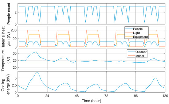
Figure 1.
Operating conditions and corresponding energy consumption.
Further, the Generator_PVWatts.idf photovoltaic (PV) example model of EnergyPlus was applied for simulation of renewable energy. It is a model developed by the National Renewable Energy Laboratory (NREL) to calculate the energy production of a PV system connected to the grid based on simple input data. The example includes one 4 kW-class PV module (PV-1) and two 3 kW-class modules (PV-2 and PV-3). The weather data for the Incheon area were also used as with the building energy model. For the tilt angle of each PV module, the initial values designated by NREL were applied. The tilt angle was set to 20° for PV-1. In the case of PV-2 and PV-3, the tilt angle was set to 37° for the Incheon area, as it follows the latitude of the analysis area. Table 1 summarizes the parameters of the PV models. More detailed performance and relations of the PV modules can be found in the references provided by NREL [33]. Figure 2 shows a schematic of the systems in the target building, including the PV modules.

Table 1.
Parameters of photovoltaic (PV) models.
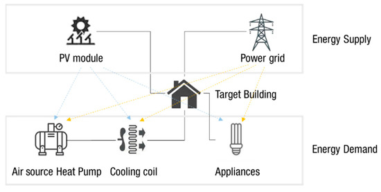
Figure 2.
Schematic of energy systems for case study building.
3. Deep Learning-Based Building Energy Model (Proposed Model)
3.1. LSTM Network
There are various deep learning models depending on the neural network structure for learning. Among them, long short-term memory (LSTM) models based on recurrent neural networks are known to be favorable for learning data with time-series characteristics or sequences [34,35]. In the building sector, various studies have also used the LSTM structure as a building load prediction model considering the time-series characteristics, in which the load occurrence pattern of the previous time affects that of the following time. The LSTM network consists of an input layer, multiple hidden layers, and an output layer. Its main characteristics lie in the memory cells of the hidden layers, and data are learned by maintaining or adjusting the status of the memory cells. A detailed description of the LSTM network can be found in previous studies [36,37,38]. The proposed LSTM model was constructed using the deep learning toolbox provided by MATLAB. For the LSTM structure, learning parameters that determine learning performance must be designated, and they are summarized in Table 2. The set values of the parameters were determined based on the values recommended by MATLAB and previous studies [39,40].
Table 2.
Parameters of long short-term memory (LSTM) model and execution environment.
3.2. Data-Driven LSTM Model
In this study, a situation in which the measured building operation data were not sufficient was assumed, and data to be used for learning were generated by simulating the EnergyPlus reference building introduced above. As for the data acquisition process, 240 (24 h × 10) set-point temperatures for 10 days were randomly generated through the Randi function, which generates random numbers through MATLAB. Here, random numbers were generated only within the ±1.5 °C range at 24 °C, which is the reference cooling set-point temperature of the reference building model. The set-point temperature data generated from MATLAB were received by EnergyPlus. After performing an energy simulation for 10 days, the simulation results were transmitted back to MATLAB. This process was repeated for 500 s based on the simulation time of MATLAB. Here, the time utilized for data collection and the energy simulation period could be extended to more than 10 days, because it is expected that the performance of the deep learning model can be improved as the number of datasets to be used for learning increases. Considering the MPC characteristics, which require that the operation plan for the following day is established rapidly, excessive simulation conditions for data collection were not set. The co-simulation toolbox provided by MATLAB was used for data communication between MATLAB and EnergyPlus. EnergyPlus transmitted and received data through an external interface. Detailed data communication through the external interface can be found in the materials provided by EnergyPlus [41]. Finally, the collected data were used as the input and target data of the LSTM model, as summarized in Table 3. The input data of the model included weather data, such as solar irradiance, the outdoor temperature, humidity, set-point temperature, and time of day (1–24 h). The output data were the energy consumption of the cooling coil.
Table 3.
Input and output of LSTM model.
4. MPC Simulation
Our MPC determines the optimal set-point temperature operation plan for a day that can minimize the grid electricity consumption considering the PV production on the following day, as shown in Equation (1).
Here, the grid electricity (Egrid) refers to the electricity consumption obtained by subtracting the PV production (EPV) from the building electricity consumption (Econsumption) that occurs at a specific time. If EPV is larger than Econsumption, EPV is regarded as the unused energy. The simulated building case does not consider the energy storage system (ESS) for surplus PV production as following a typical family house case. Thus, the reduction effect of the surplus PV energy is indirectly included in the objective function.
The proposed data-based model was applied for the MPC. An attempt was made to compare it with the detailed analysis program model, which is the reference model. In this study, an optimization algorithm was applied to the two developed building energy models, and the optimization results and simulation time were comprehensively analyzed.
The particle swarm optimization (PSO) algorithm was employed for the optimization algorithm. The PSO algorithm, an algorithm for finding the optimal solution based on the social behavior in a cluster, was first proposed by Eberhart and Kennedy [42]. According to Zhang et al. [43], PSO is one of the most commonly used optimization algorithms. It has been widely applied in numerous areas, owing to its simple algorithm and short computation time [44,45]. In this study, the PSO algorithm with relatively fast computation time was employed, considering the characteristics of MPC in which the operation strategy for the following day must be rapidly established. The swarm size, a main set value that determines the performance of PSO, was set to 2400. For the other set values of PSO, the values recommended by previous studies and MATLAB were applied.
It was also assumed that the PV usage and weather were perfectly predicted from previous studies [46,47]. In ASHRAE standard 55, the range of set temperatures for comfort is specified as 22.2 to 25.5 °C [48], and following this standard, the bounds of temperatures for applying PSO are set from 22.5 to 25.5 °C. Figure 3 shows the PSO process of the proposed two building models and the comparison process through simulation.
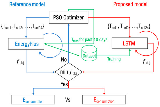
Figure 3.
Proposed day ahead scheduling algorithm optimized by particle swarm optimization (PSO) (reference vs. LSTM).
The simulation was performed for six days from 6 August to 11 August during the cooling period. The errors were analyzed using RMSE and CVRMSE, which are typical error evaluation methods expressed in Equations (2) and (3).
5. Simulation Results
5.1. LSTM Model Verification
As previously mentioned, the proposed LSTM model learns the EnergyPlus simulation results for the past 10 days according to the arbitrarily determined set-point temperature. Here, if the energy use patterns for the past 10 days, which are the training data of the model, are similarly described, it can be expected that the accuracy of predicting the building energy consumption for the following day, which is the prediction target, will increase.
In this study, building energy models were developed for six days, from 6 August 2020 to 11 August 2020. The learning models learned building energy use patterns for 275 set-point temperature scenarios on average, over the simulation time of 500 s, and the learning error for six days was only 28 Wh (CVRMSE 3.7%). Figure 4 shows the results of comparison of the learning period with the largest error in learning performance and the period with the smallest error. For both models, most of the points were distributed on the diagonal line and errors of CVRMSE 5.3% and 2.8% were observed, respectively, resulting in no significant difference. Table 4 summarizes the learning errors of the proposed model.
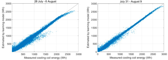
Figure 4.
Learning performance: cooling coil energy consumption per area for prediction on 7 August 2020 and 10 August 2020.
Table 4.
Learning and prediction error of proposed model.
Figure 5 shows the results of predicting the daily building energy consumption for the proposed model. For model evaluation, the set-point temperature for 24 h on the following day was determined through the Randi function in MATLAB, and subsequently the results of applying the same set-point temperature to the reference and proposed models were compared. The proposed model described energy use patterns similar to those of the reference model for the six days of the test, and exhibited errors of RMSE 127 Wh and CVRMSE 14% each day on average. Considering that the peak energy consumption during the test period was approximately 3 kW, it appears that the proposed model can be sufficiently used as a building energy model for MPC. Most of the errors of the model occurred in the early morning when energy consumption was low, and the error was only 10% from 07:00 to 18:00, which is the time zone for main energy use. Table 4 summarizes the prediction performance of each model.
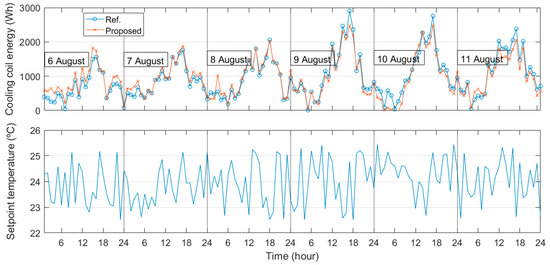
Figure 5.
Prediction performance: cooling coil energy consumption.
Figure 6 shows the learning and prediction performances for an extended period of 1 August 2020 to 31 August 2020. This is achieved for further model verification. The left side of the figure shows the learning performance, and the right side shows the prediction performance of the model. CVRMSE for learning was 6.9% and 16.9% for prediction, and the results are similar to the sample period as given in Table 4.
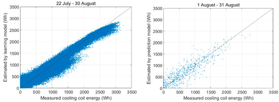
Figure 6.
Learning and prediction performance for predicting an entire month of August.
5.2. Optimization Simulation Results
Figure 7 shows the set-point temperatures and energy consumption derived as PSO optimization results. The proposed and reference models performed a planning of daily set-point temperatures that minimize the objective function through PSO and applied the results. First of all, the proposed model considered the PV power generation time on the third and fourth days of simulation, and showed cooling operation patterns, in which the set-point temperature was decreased during daytime when the amount of power generated was large and increased in the evening and early morning. On the fourth day, in particular, it yielded a scenario that reduced the grid electricity consumption by more than 4 kWh compared to the reference model. The two models did not also provide completely identical set-point scenarios in other periods. Based on the finding that the cooling coil energy consumption itself was similar for the two models as shown in the upper graph in Figure 6, it was confirmed that similar amounts of energy were used to handle the indoor heating load, regardless of the change in set-point temperature.
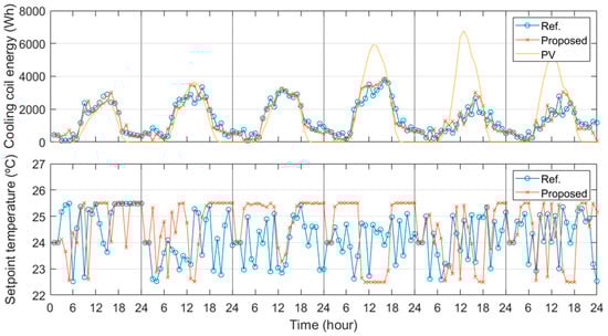
Figure 7.
Comparison of optimized operating results (reference vs. proposed).
Figure 8 shows the daily grid energy consumption. In the figure, the bar graph labeled ‘fixed-setpoint control’ represents an EnergyPlus simulation in which a fixed-setpoint temperature of 24 °C was applied. There is no difference in the energy used by the cooling coil between the models, as the purpose of the energy is to handle the building load. However, if a plan is established to maximize the utilization of renewable energy, the energy actually used becomes different, as the grid electricity consumption can be reduced.
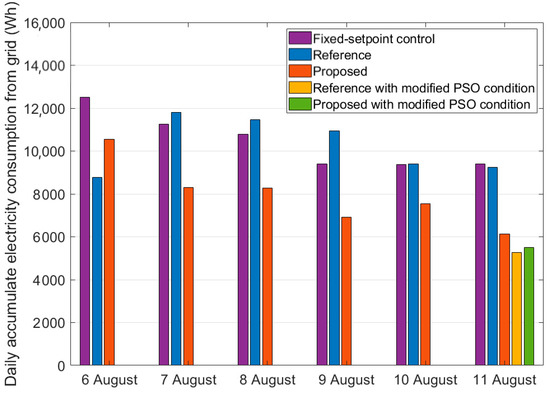
Figure 8.
Comparison of daily grid energy consumption (reference vs. proposed).
In the figure, the proposed model used less energy in all sections except for 6 August 2020. The error on 6 August 2020 was caused by the performance of the model. As shown in the previous model evaluation in Table 4, it was difficult to obtain meaningful optimization simulation results on 6 August 2020, because the performance prediction error of the model was relatively large. From 7 August 2020 to 11 August 2020, the operation scenario by the proposed model could save grid energy consumption by more than 35% (2.9 kWh) each day on average compared to the reference case. The MPC scenario increased self-consumption of PV energy and reduced PV curtailment.
However, it can be interpreted that it was difficult for the reference model to find the optimal solution, even though it used the same PSO technique in this study. The reference model consumed approximately 100 min on average until the completion of simulation, because it performed co-simulation with EnergyPlus at every iteration.
In contrast, the proposed model yielded better optimization results in the process of executing it and obtaining the results despite the same PSO option, because it is a lightweight network model that can perform optimization simulation without communication with a separate external program after its construction. It consumed only approximately 30 min on average for the simulation, even including the process of extracting data from EnergyPlus for learning.
The bar graph added on 11 August 2020 in Figure 8 shows the result of performing the PSO optimization of the reference model by removing the Maxtime boundary among the PSO optimization options for a day. The result provided a set-point temperature scenario that reduced energy consumption by approximately 43% compared to the initial reference simulation result. In this instance, the energy consumption pattern was very similar to that of the proposed model, as shown in Figure 9, and the grid energy consumption was also reduced by more than 9% compared to the proposed model. Similarly, when the Maxtime boundary was removed for the proposed model, the model gave a reduced energy consumption by 1.4% compared to the case without modified PSO conditions.
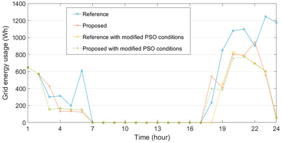
Figure 9.
Comparison of optimization results on 11 August 2020.
Figure 10 shows the simulation results and corresponding CPU time on 11 August 2020. according to limited and unlimited PSO conditions. As can be seen from Figure 8 and Figure 9, the proposed model showed very similar energy simulation results to the modified PSO conditions cases. This means that optimization with the proposed model can sufficiently converge with the limited Maxtime condition. However, in terms of simulation time, it took only 22 min while other cases with modified PSO conditions needed more simulation time. This indicates that it will be difficult to actually apply the reference model to the test environment of this study with ensuring convergence, considering the characteristics of MPC in which the operation plan for the following day is established at 23:00 on the previous day, or real-time control is performed.
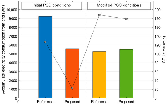
Figure 10.
Comparison of grid energy consumption and simulation run time on 11 August 2020.
Figure 11 shows the unused PV energy, which is due to the surplus of PV production compared to required energy consumption. Thus, lower values mean higher efficiency of the proposed operating strategies. This can be an important factor to evaluate the MPC performance for typical houses without resorting to ESS. From Figure 11, the difference in unused PV energy between the reference and proposed model is about 1.8 kWh, so 3.7 kWh, the difference in Egrid between models, attributes the reduction effect of the unused PV energy. The other effect is surely optimized indoor setpoint temperatures.
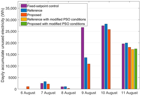
Figure 11.
Comparison of daily unused PV energy.
For the case of 9 August 2020, the MPC models utilized the produced PV energy at a similar level while the fixed-setpoint control used less PV energy. This can be interpreted that the MPC models maximize cooling load by lowering setpoint temperatures during the daytime. On average, the reference and proposed models consumed PV energy more than the fixed-set point control by 1.8 and 3.1 kWh, respectively, for a day.
Table 5 summarizes the detailed simulation results, including grid energy consumption, average indoor temperature, unused PV energy, and simulation time.
Table 5.
Model predictive control (MPC) results of test models.
6. Conclusions
A long short-term memory (LSTM)-based building energy model, which learns the data obtained from a detailed building energy model, was proposed as a predictive control of a building. The operation scenario to reduce the grid electricity consumption on the following day was derived by applying the PSO algorithm to the proposed model. The LSTM-based building model was developed to predict the energy consumption of the building according to the set-point temperature and to establish the optimal set-point temperature plan that minimizes the use of electrical energy during the test period through a combination with the optimization algorithm. A verification test was conducted between the proposed and the reference building energy model. The energy consumption prediction performance of CVRMSE 12% was observed on average, indicating that the proposed model can be used as a building energy model for MPC.
The MPC simulation results showed that the proposed model could reduce the average daily grid energy consumption by approximately 30% compared to the reference model for most of the period. Partly, the proposed model utilized more PV energy produced, and it means that the model reduced unused PV energy.
A main advantage of the proposed MPC model is that it is possible to speed up the simulation for applicable MPC implementation. The average daily simulation time consumed was approximately 30 min for the proposed model, whereas it was approximately 100 min for the reference model. This means that sufficient optimization may not be achieved, depending on the computation time of the target model, even if the same optimization function is used. This may affect the performance degradation of MPC, which must establish the operation plan for the following day within a limited time.
For buildings with insufficient measurement data, MPC can be implemented through a well-fitted detailed building energy model. It is difficult, however, for the detailed model to achieve sufficient optimization within a given time, because it requires a long computation time for optimization, as seen from the results. The proposed model demonstrated better performance compared to the reference model. As the data-based model is significantly affected by the training data, training was performed by extracting daily model behavior according to the weather data and operating conditions for the past few days. If sufficient data for MPC are secured as the operation continues, however, there will be benefits in terms of model usability, as the appropriately trained model without sequencing may be used only for the optimization process, thus significantly reducing the time required.
Author Contributions
All authors developed and tested the presented models and methodologies. B.-K.J. drafted this manuscript, E.-J.K. revised it, and all authors approved the current manuscript. All authors have read and agreed to the published version of the manuscript.
Funding
This work was supported by the Korea Institute of Energy Technology Evaluation and Planning (KETEP) grant funded by the Korean government (MOTIE) (2019271010015D, Development of Smart city Energy Business Service).
Institutional Review Board Statement
Not applicable.
Informed Consent Statement
Not applicable.
Data Availability Statement
No new data were created or analyzed in this study. Data sharing is not applicable to this article.
Conflicts of Interest
The authors declare no conflict of interest.
Nomenclature
| Symbol | Subscript |
| f | function |
| Econsumption | Electricity consumption (Wh) |
| Egrid | Grid electricity consumption (Wh) |
| EPV | PV electricity production (Wh) |
| T | temperature (°C) |
| t | time (s) |
| v | value |
| obj | object |
| ref. | reference |
| t | time (hour) |
References
- Zhuang, J.; Chen, Y.; Chen, X. A new simplified modeling method for model predictive control in a medi-um-sized commercial building: A case study. Build. Environ. 2018, 127, 1–12. [Google Scholar] [CrossRef]
- Henze, G.P.; Felsmann, C.; Knabe, G. Evaluation of optimal control for active and passive building thermal storage. Int. J. Therm. Sci. 2004, 43, 173–183. [Google Scholar] [CrossRef]
- Verhelst, C.; Logist, F.; Van Impe, J.; Helsen, L. Study of the optimal control problem formulation for modulat-ing air-to-water heat pumps connected to a residential floor heating system. Energy Build. 2012, 45, 43–53. [Google Scholar] [CrossRef]
- Mbungu, N.T.; Naidoo, R.M.; Bansal, R.C. Real-time electricity pricing: TOU-MPC based energy manage-ment for commercial buildings. Energy Procedia 2017, 105, 3419–3424. [Google Scholar] [CrossRef]
- Joe, J.; Im, P.; Dong, J. Empirical modeling of direct expansion (DX) cooling system for multiple research use cases. Sustainability 2020, 12, 8738. [Google Scholar] [CrossRef]
- Ma, Y.; Borrelli, F.; Hencey, B.; Coffey, B.; Bengea, S.; Haves, P. Model Predictive Control for the Operation of Building Cooling Systems. IEEE Trans. Control. Syst. Technol. 2012, 20, 796–803. [Google Scholar]
- Prívara, S.; Široký, J.; Ferkl, L.; Cigler, J. Model predictive control of a building heating system: The first expe-rience. Energy Build. 2011, 43, 564–572. [Google Scholar] [CrossRef]
- Široký, J.; Oldewurtel, F.; Cigler, J.; Prívara, S. Experimental analysis of model predictive control for an energy efficient building heating system. Appl. Energy 2011, 88, 3079–3087. [Google Scholar] [CrossRef]
- Gyalistras, D.; Gwerder, M. Use of Weather and Occupancy Forecasts for Optimal Building Climate Control (Op-tiControl): Two Years Progress Report; Terrestrial Systems Ecology; ETH Zürich: Zürich, Switzerland; Building Technologies Division, Siemens Switzerland Ltd.: Zug, Switzerland, 2010. [Google Scholar]
- Nguyen, T.-T.; Yoo, H.-J.; Kim, H.-M. Analyzing the Impacts of System Parameters on MPC-Based Frequency Control for a Stand-Alone Microgrid. Energies 2017, 10, 417. [Google Scholar] [CrossRef]
- Afram, A.; Janabi-Sharifi, F. Theory and applications of HVAC control systems—A review of model predictive control (MPC). Build. Environ. 2014, 72, 343–355. [Google Scholar] [CrossRef]
- Khanmirza, E.; Esmaeilzadeh, A.; Markazi, A.H.D. Predictive control of a building hybrid heating system for energy cost reduction. Appl. Soft Comput. 2016, 46, 407–423. [Google Scholar] [CrossRef]
- Prívara, S.; Váňa, Z.; Žáčeková, E.; Cigler, J. Building modeling: Selection of the most appropriate model for predictive control. Energy Build. 2012, 55, 341–350. [Google Scholar] [CrossRef]
- Hoes, P.; Loonen, R.C.G.M.; Trcka, M.; Hensen, J. Performance Prediction of Advanced Building Controls in the Design Phase Using ESP-r, BCVTB and MATLAB; BSO12 (IBPSA-England): Loughborough, UK, 2012. [Google Scholar]
- Zhao, J.; Lam, K.P.; Ydstie, B.E.; Loftness, V. Occupant-oriented mixed-mode EnergyPlus predictive control simulation. Energy Build. 2016, 117, 362–371. [Google Scholar] [CrossRef]
- Hilliard, T.; Swan, L.; Kavgic, M.; Qin, Z. Applying model predictive control to a LEED silver-certified build-ing. Energy Procedia 2015, 78, 1817–1822. [Google Scholar] [CrossRef]
- Bruni, G.; Cordiner, S.; Mulone, V.; Rocco, V.; Spagnolo, F. A study of energy management in domestic mi-cro-grids based on model predictive control strategies. Energy Procedia 2014, 61, 1012–1016. [Google Scholar] [CrossRef]
- Afram, A.; Janabi-Sharifi, F.; Fung, A.S.; Raahemifar, K. Artificial neural network (ANN) based model predic-tive control (MPC) and optimization of HVAC systems: A state of the art review and case study of a residential HVAC system. Energy Build. 2017, 141, 96–113. [Google Scholar] [CrossRef]
- Dounis, A.; Caraiscos, C. Advanced control systems engineering for energy and comfort management in a building environment—A review. Renew. Sustain. Energy Rev. 2009, 13, 1246–1261. [Google Scholar] [CrossRef]
- Huang, H.; Chen, L.; Hu, E. A new model predictive control scheme for energy and cost savings in commercial buildings: An airport terminal building case study. Build. Environ. 2015, 89, 203–216. [Google Scholar] [CrossRef]
- Lu, L.; Cai, W.; Xie, L.; Li, S.; Soh, Y.C. HVAC system optimization—In-building section. Energy Build. 2005, 37, 11–22. [Google Scholar] [CrossRef]
- Ning, M.; Zaheeruddin, M. Neuro-optimal operation of a variable air volume HVAC&R system. Appl. Therm. Eng. 2010, 30, 385–399. [Google Scholar]
- Kusiak, A.; Xu, G.; Tang, F. Optimization of an HVAC system with a strength multi-objective particle-swarm algorithm. Energy 2011, 36, 5935–5943. [Google Scholar] [CrossRef]
- Kusiak, A.; Xu, G.; Zhang, Z. Minimization of energy consumption in HVAC systems with data-driven models and an interior-point method. Energy Convers. Manag. 2014, 85, 146–153. [Google Scholar] [CrossRef]
- Weron, R. Electricity price forecasting: A review of the state-of-the-art with a look into the future. Int. J. Forecast. 2014, 30, 1030–1081. [Google Scholar] [CrossRef]
- Kim, M.; Hong, C. The Artificial Neural Network based Electric Power Demand Forecast using a Season and Weather Informations. J. Inst. Electron. Inf. Eng. 2016, 53, 71–78. [Google Scholar]
- Li, X.; Wen, J. Review of building energy modeling for control and operation. Renew. Sustain. Energy Rev. 2014, 37, 517–537. [Google Scholar] [CrossRef]
- Fabrizio, E.; Monetti, V. Methodologies and advancements in the calibration of building energy mod-els. Energies 2015, 8, 2548–2574. [Google Scholar] [CrossRef]
- Taheri, M.; Tahmasebi, F.; Mahdavi, A. A case study of optimization-aided thermal building performance sim-ulation calibration. Optimization 2012, 4, 603–607. [Google Scholar]
- Kim, W.; Jeon, Y.; Kim, Y. Simulation-based optimization of an integrated daylighting and HVAC system using the design of experiments method. Appl. Energy 2016, 162, 666–674. [Google Scholar] [CrossRef]
- Shin, Y.; Kim, E.-J.; Lee, K.-H. Optimal Cooling Operation of a Single Family House Model Equipped with Renewable Energy Facility by Linear Programming. Korean J. Air Cond. Refrig. Eng. 2017, 29, 638–644. [Google Scholar]
- Jeon, B.-K.; Kim, E.-J.; Shin, Y.; Lee, K.-H. Learning-Based Predictive Building Energy Model Using Weather Forecasts for Optimal Control of Domestic Energy Systems. Sustainability 2018, 11, 147. [Google Scholar] [CrossRef]
- Dobos, A.P. PVWatts Version 5 Manual; National Renewable Energy Lab. (NREL): Golden, CO, USA, 2014.
- Schuster, M.; Paliwal, K. Bidirectional recurrent neural networks. IEEE Trans. Signal Process. 1997, 45, 2673–2681. [Google Scholar] [CrossRef]
- Hochreiter, S.; Schmidhuber, J. Long Short-Term Memory. Neural Comput. 1997, 9, 1735–1780. [Google Scholar] [CrossRef] [PubMed]
- Somu, N.; MR, G.R.; Ramamritham, K. A hybrid model for building energy consumption forecasting us-ing long short term memory networks. Appl. Energy 2020, 261, 114131. [Google Scholar] [CrossRef]
- Muzaffar, S.; Afshari, A. Short-Term Load Forecasts Using LSTM Networks. Energy Procedia 2019, 158, 2922–2927. [Google Scholar] [CrossRef]
- Kim, T.-Y.; Cho, S.-B. Predicting residential energy consumption using CNN-LSTM neural networks. Energy 2019, 182, 72–81. [Google Scholar] [CrossRef]
- Documentation, M.A.T.L.A.B. Matlab Documentation. Matlab, R2012b. 2012. Available online: https://www.mathworks.com/help/matlab/ (accessed on 17 January 2021).
- Kingma, D.P.; Ba, J. Adam: A method for stochastic optimization. In Proceedings of the International Conference Learn, Represent, (ICLR), San Diego, CA, USA, 5–8 May 2015. [Google Scholar]
- Guide, A. Guide for Using EnergyPlus with External Interface (s); US Department of Energy: Washington, DC, USA, 2011.
- Kennedy, J.; Eberhart, R. Particle swarm optimization. In Proceedings of the ICNN’95-International Conference on Neural Networks, Perth, WA, Australia, 27 November–1 December 1995; Volume 4, pp. 1942–1948. [Google Scholar]
- Zhang, Y.; Wang, S.; Ji, G. A comprehensive survey on particle swarm optimization algorithm and its applica-tions. Math. Probl. Eng. 2015, 2015, 1–38. [Google Scholar]
- Wu, X.; Dai, J.; Zhao, Y.; Zhuo, Z.; Yang, J.; Zeng, X.C. Two-Dimensional Boron Monolayer Sheets. ACS Nano 2012, 6, 7443–7453. [Google Scholar] [CrossRef]
- Tambouratzis, G. Using Particle Swarm Optimization to Accurately Identify Syntactic Phrases in Free Text. J. Artif. Intell. Soft Comput. Res. 2018, 8, 63–77. [Google Scholar] [CrossRef]
- Jeon, B.-K.; Kim, E.-J. Next-Day Prediction of Hourly Solar Irradiance Using Local Weather Forecasts and LSTM Trained with Non-Local Data. Energies 2020, 13, 5258. [Google Scholar] [CrossRef]
- Lu, H.; Chang, G.W. A Hybrid Approach for Day-Ahead Forecast of PV Power Generation. IFAC PapersOnLine 2018, 51, 634–638. [Google Scholar] [CrossRef]
- Ashrae, A. ANSI/ASHRAE 55–2010 Thermal Environmental Conditions for Human Occupancy; American Society of Heating, Refrigerating and Air-Conditioning Engineering: Atlanta, GA, USA, 2010. [Google Scholar]


Publisher’s Note: MDPI stays neutral with regard to jurisdictional claims in published maps and institutional affiliations. |
© 2021 by the authors. Licensee MDPI, Basel, Switzerland. This article is an open access article distributed under the terms and conditions of the Creative Commons Attribution (CC BY) license (http://creativecommons.org/licenses/by/4.0/).