Prediction of Land Use and Land Cover Changes in Mumbai City, India, Using Remote Sensing Data and a Multilayer Perceptron Neural Network-Based Markov Chain Model


Abstract
1. Introduction
1.1. Land Use and Land Cover
1.2. LULC Simulation and Prediction
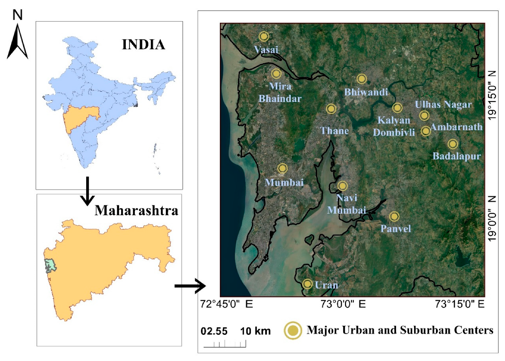
2. Study Area and Material
2.1. Study Area
2.2. Data
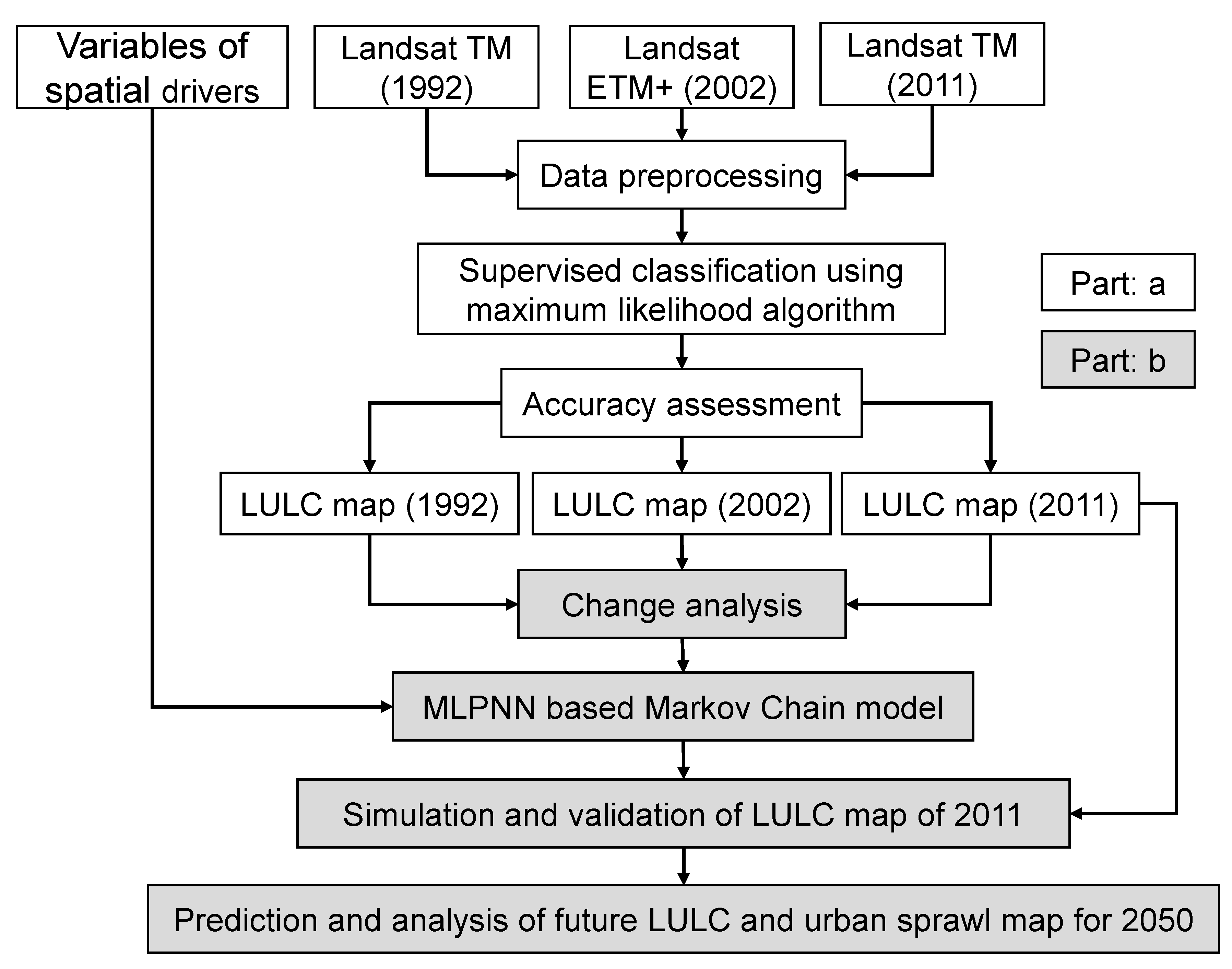
3. Methodology
3.1. Image Preprocessing and Classification
3.2. Accuracy Assessment of LULC Classification
3.3. Prediction of Future LULC Pattern
3.3.1. LULC Change Analysis
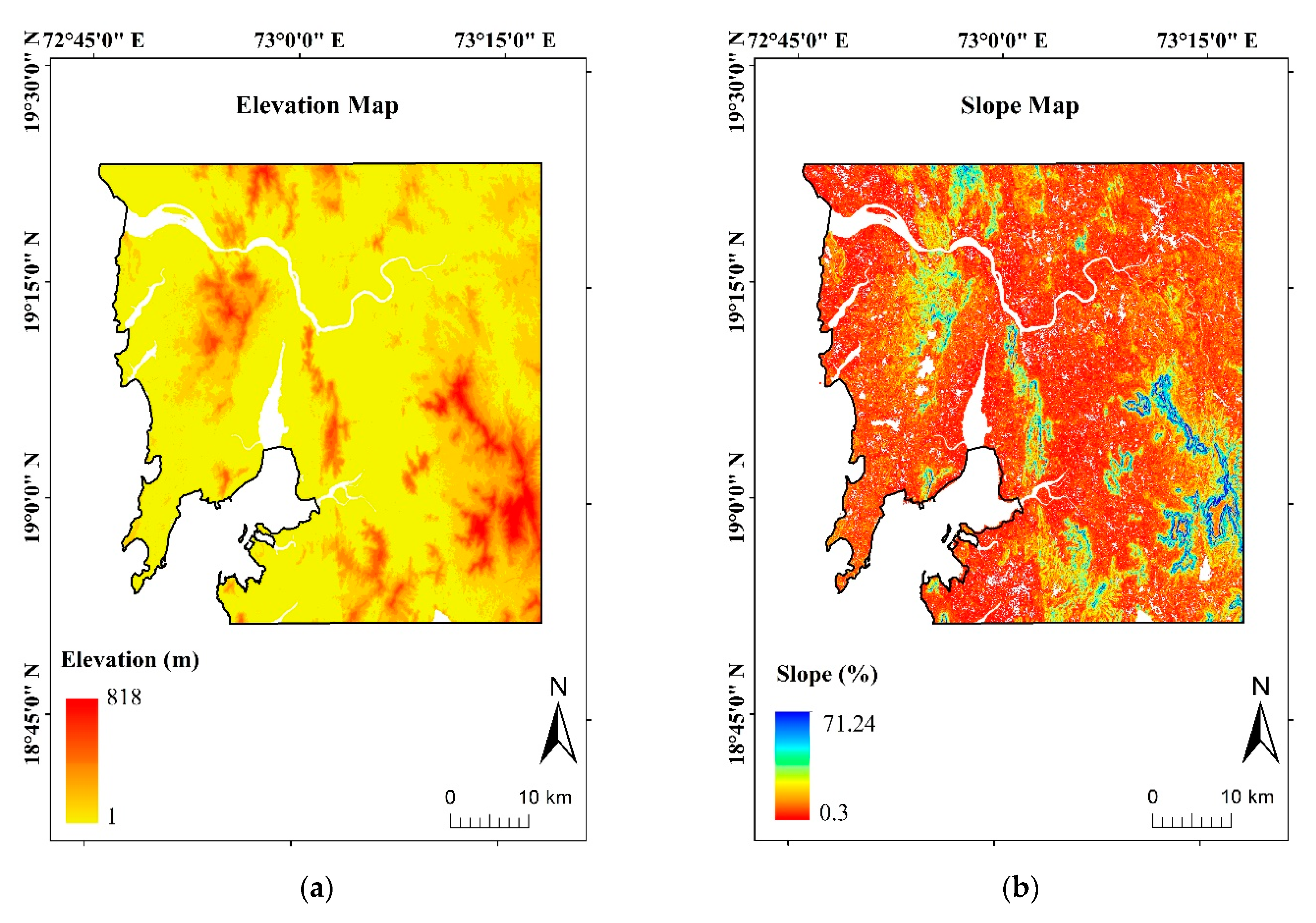
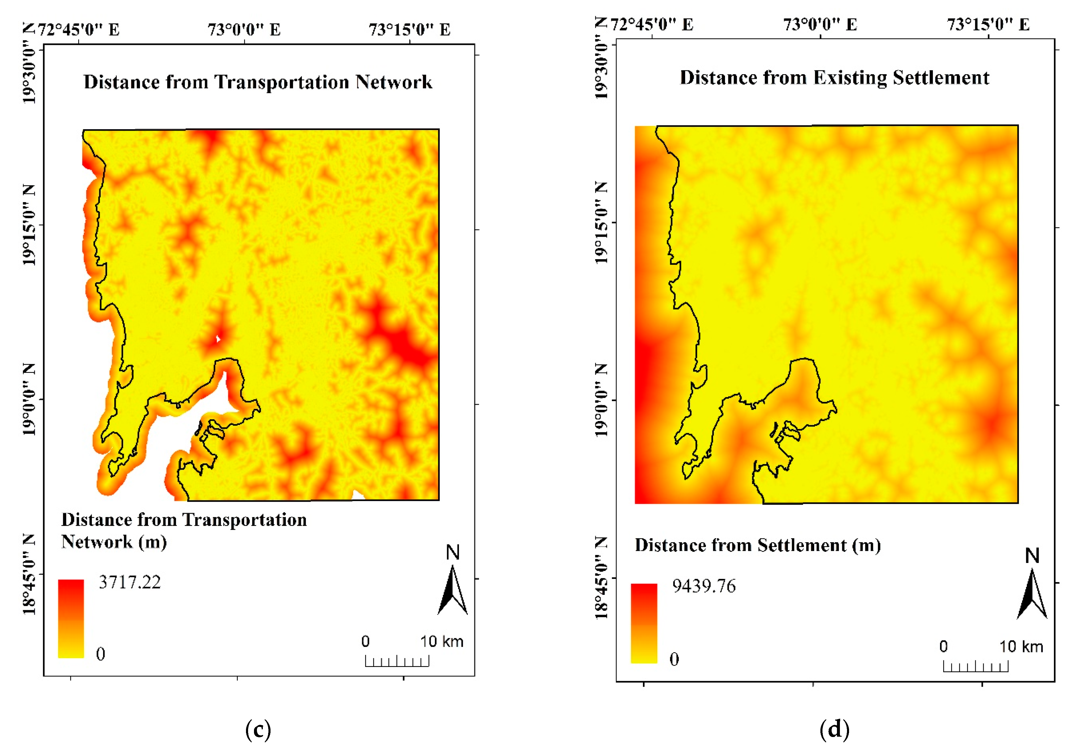
3.3.2. Evaluation and Selection of Spatial Drivers
3.3.3. Preparation of Transition Potential
3.3.4. LULC Prediction and Validation
4. Results and Discussion
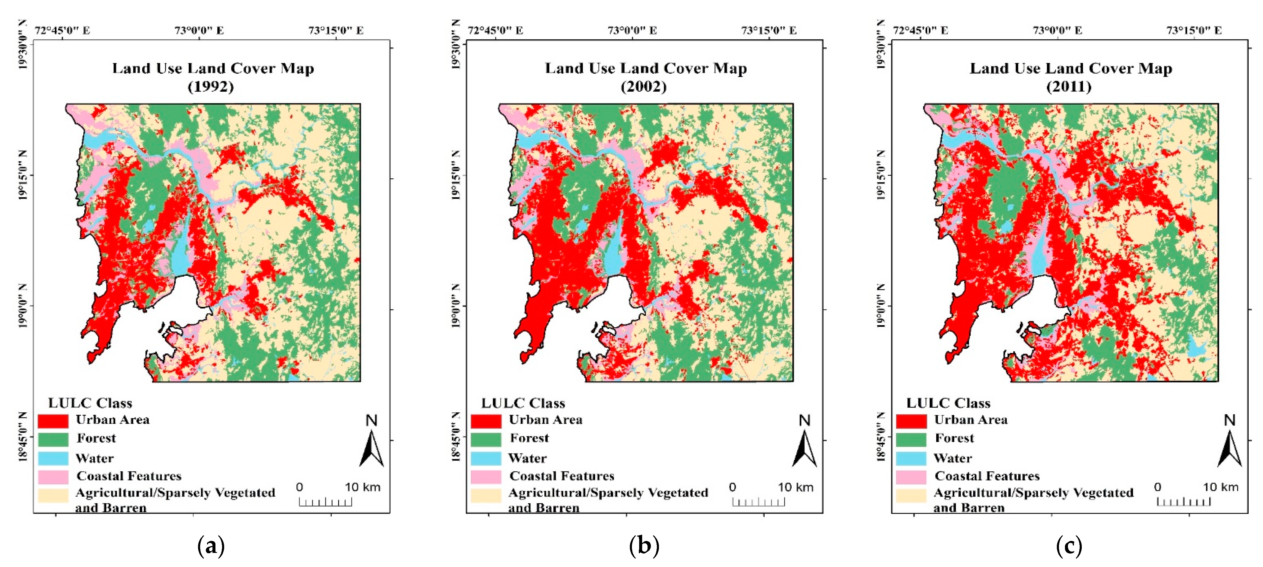
4.1. LULC Classification and Accuracy Assessment
4.2. Analysis of Change Detection
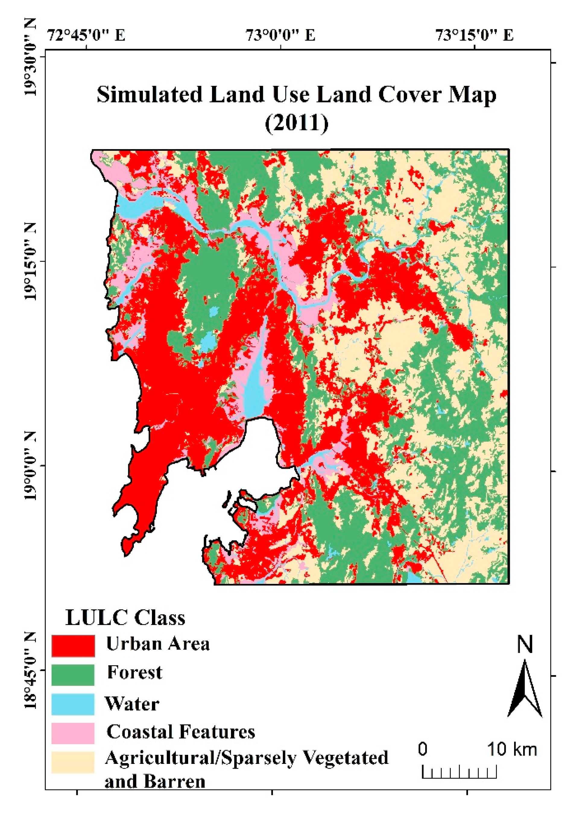
4.3. Prediction and Validation of 2011 LULC
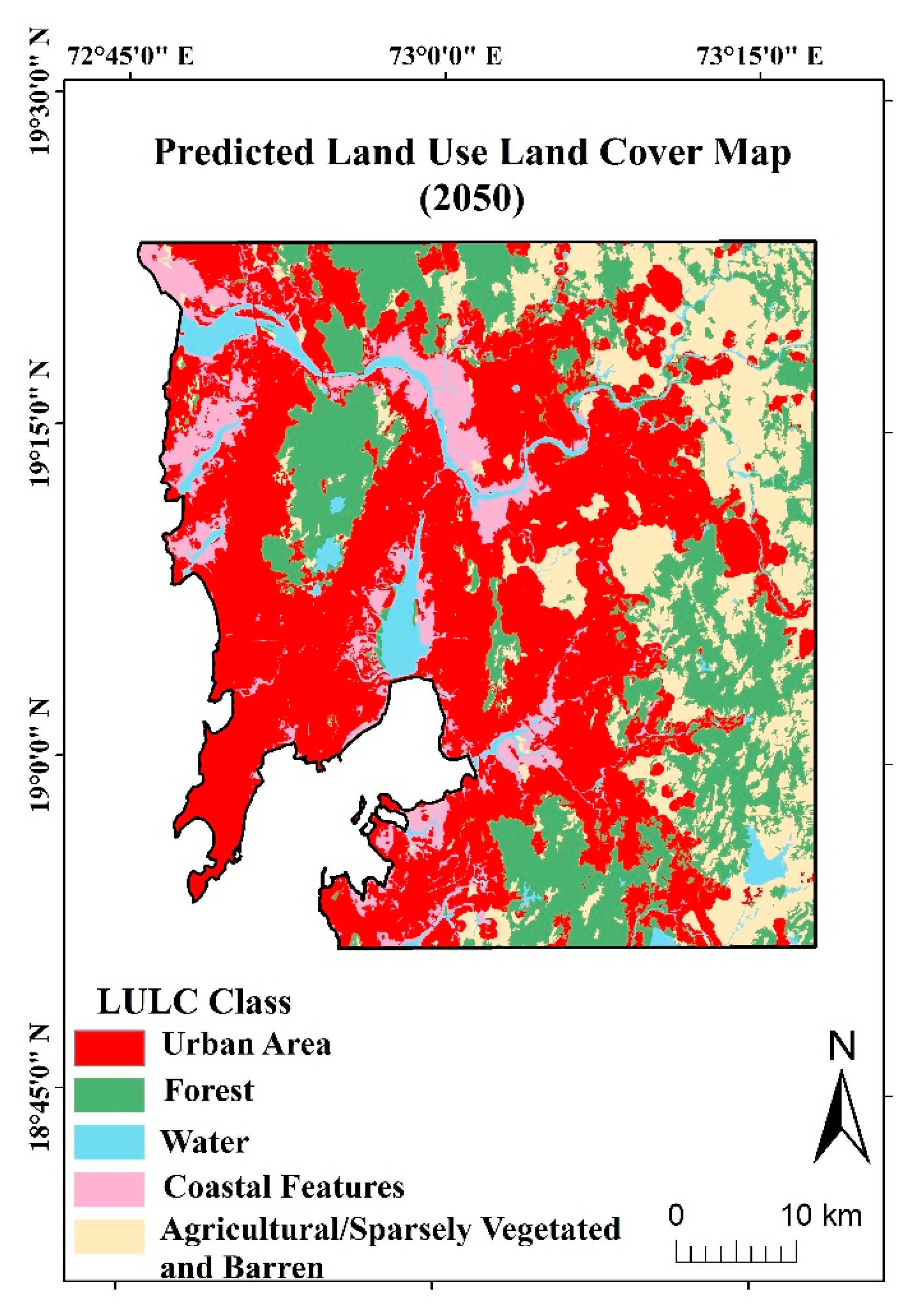
4.4. Prediction of 2050 LULC
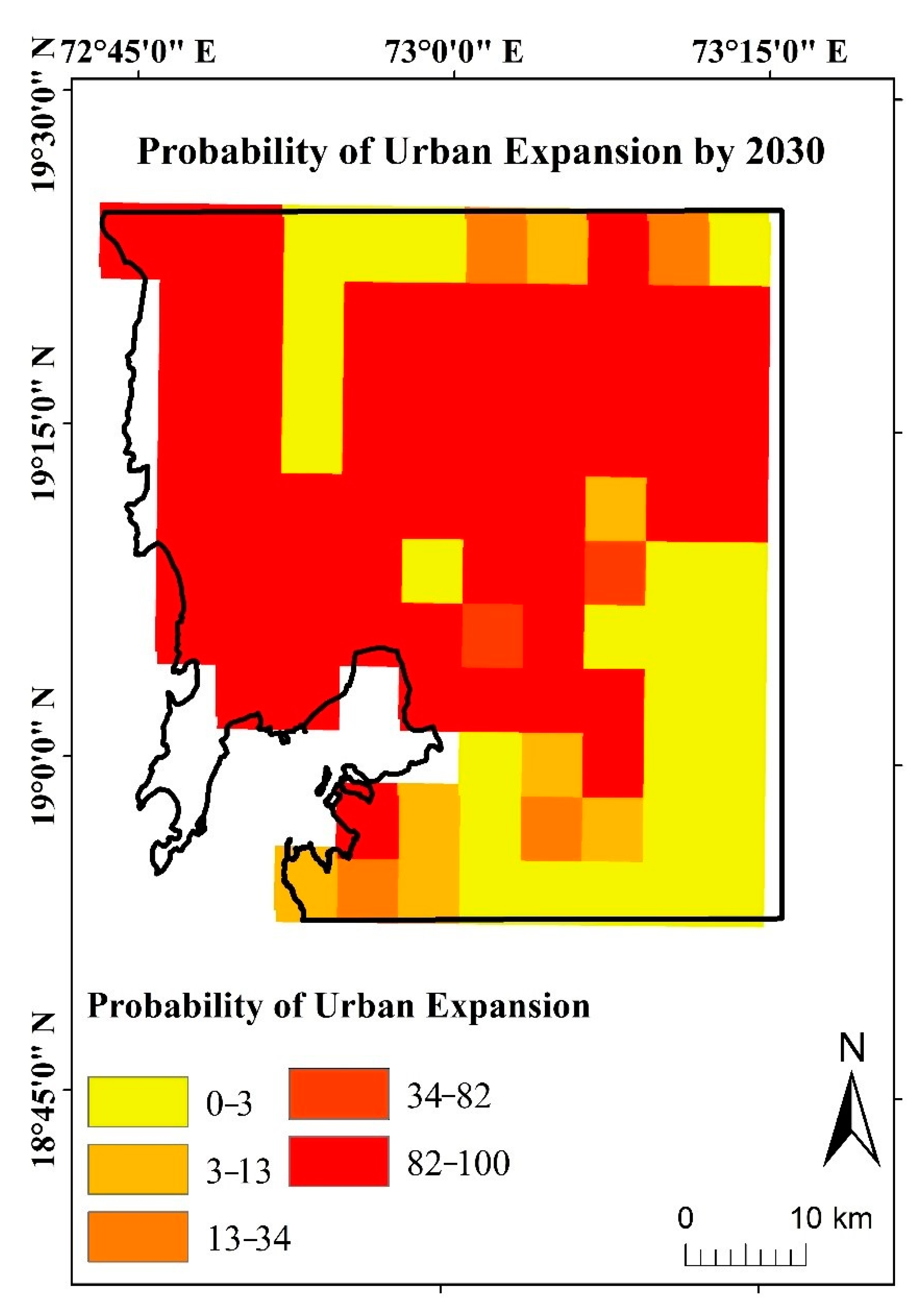
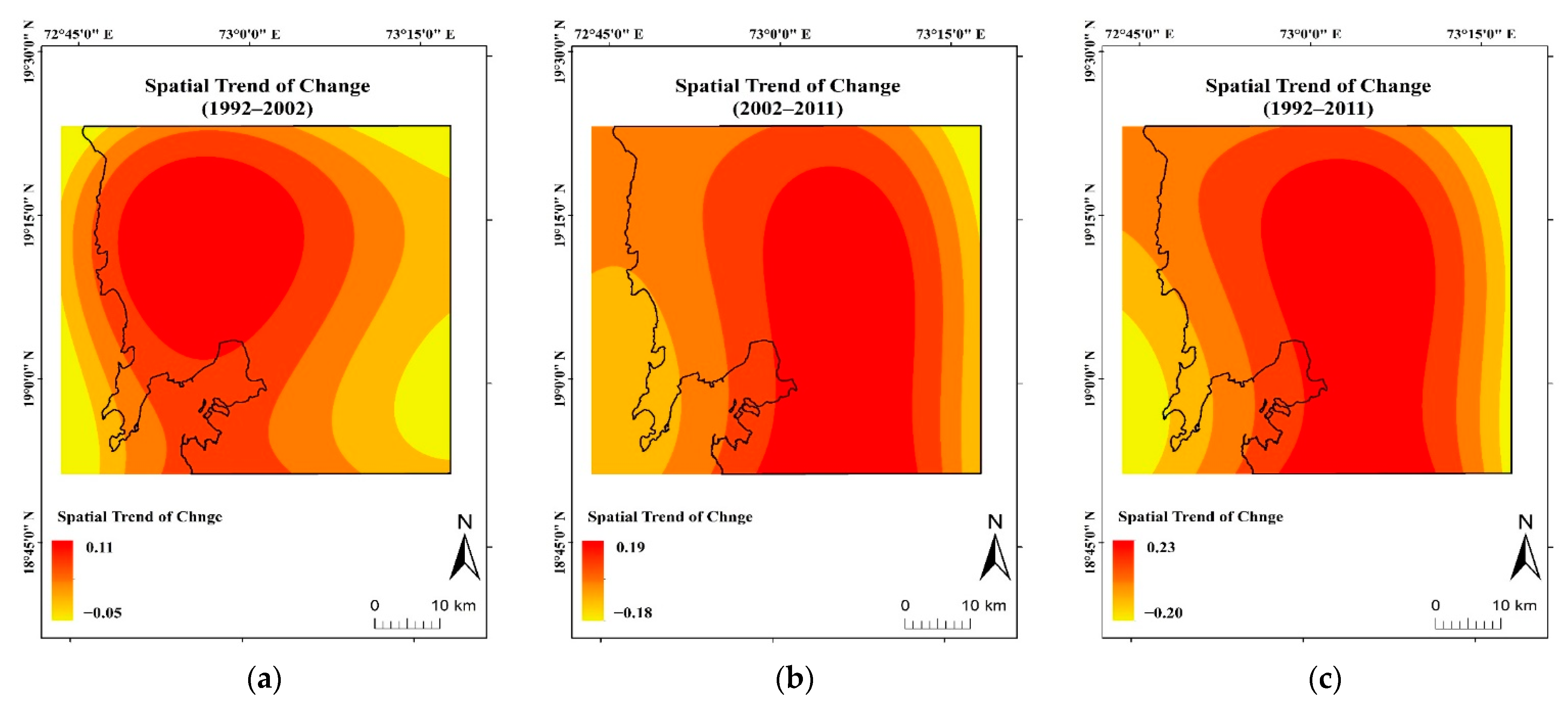
4.5. Spatial Trend of Urban Growth
5. Conclusions
Author Contributions
Funding
Institutional Review Board Statement
Informed Consent Statement
Data Availability Statement
Acknowledgments
Conflicts of Interest
Appendix A

| Type of Kappa Coefficient | Description |
|---|---|
| Kappa for no-information (kno) | kno is the ratio among accurately classified pixels to the anticipated proportion of pixels |
| Kappa for grid-cell-location (klocation) | It represents the spatial-level correctness associated with the level of location-wise agreement |
| Cohen’s Kappa statistics (kstandard) | kstandard is the proportion of accurately assigned pixels to the proportion may be accurate by chance |
| Kappa for stratum-level-location (klocation strata) | klocation strata is an accuracy-related with the accurate assignment predefined strata |
References
- Hassan, Z.; Shabbir, R.; Ahmad, S.S.; Malik, A.H.; Aziz, N.; Butt, A.; Erum, S. Dynamics of land use and land cover change (LULCC) using geospatial techniques: A case study of Islamabad Pakistan. SpringerPlus 2016, 5. [Google Scholar] [CrossRef] [PubMed]
- Matlhodi, B.; Kenabatho, P.K.; Parida, B.P.; Maphanyane, J.G. Evaluating land use and land cover change in the Gaborone dam catchment, Botswana, from 1984–2015 using GIS and remote sensing. Sustainability 2019, 11, 5174. [Google Scholar] [CrossRef]
- Cihlar, J. Land cover mapping of large areas from satellites: Status and research priorities. Int. J. Remote Sens. 2000, 21, 1093–1114. [Google Scholar] [CrossRef]
- Vitousek, P.M.; Mooney, H.A.; Lubchenco, J.; Melillo, J.M. Human domination of Earth’s ecosystems. Science 1997, 277, 494–499. [Google Scholar] [CrossRef]
- Shi, G.; Jiang, N.; Yao, L. Land use and cover change during the rapid economic growth period from 1990 to 2010: A case study of Shanghai. Sustainability 2018, 10, 426. [Google Scholar] [CrossRef]
- Paul, S.; Ghosh, S.; Mathew, M.; Devanand, A.; Karmakar, S.; Niyogi, D. Increased Spatial Variability and Intensification of Extreme Monsoon Rainfall due to Urbanization. Sci. Rep. 2018, 8, 1–10. [Google Scholar] [CrossRef]
- Gogoi, P.P.; Vinoj, V.; Swain, D.; Roberts, G.; Dash, J.; Tripathy, S. Land use and land cover change effect on surface temperature over Eastern India. Sci. Rep. 2019, 9, 1–10. [Google Scholar] [CrossRef]
- Zhong, S.; Qian, Y.; Zhao, C.; Leung, R.; Wang, H.; Yang, B.; Fan, J.; Yan, H.; Yang, X.Q.; Liu, D. Urbanization-induced urban heat island and aerosol effects on climate extremes in the Yangtze River Delta region of China. Atmos. Chem. Phys. 2017, 17, 5439–5457. [Google Scholar] [CrossRef]
- Deshmukh, D.S.; Chaube, U.C.; Ekube Hailu, A.; Aberra Gudeta, D.; Tegene Kassa, M. Estimation and comparision of curve numbers based on dynamic land use land cover change, observed rainfall-runoff data and land slope. J. Hydrol. 2013, 492, 89–101. [Google Scholar] [CrossRef]
- Xu, X.; Xie, Y.; Qi, K.; Luo, Z.; Wang, X. Detecting the response of bird communities and biodiversity to habitat loss and fragmentation due to urbanization. Sci. Total Environ. 2018, 624, 1561–1576. [Google Scholar] [CrossRef]
- Mortoja, M.G.; Yigitcanlar, T. Local drivers of anthropogenic climate change: Quantifying the impact through a remote sensing approach in Brisbane. Remote Sens. 2020, 12, 2270. [Google Scholar] [CrossRef]
- Mortoja, M.G.; Yigitcanlar, T. How Does Peri-Urbanization Trigger Climate Change Vulnerabilities? An Investigation of the Dhaka Megacity in Bangladesh. Remote Sens. 2020, 12, 3938. [Google Scholar] [CrossRef]
- Xystrakis, F.; Psarras, T.; Koutsias, N. A process-based land use/land cover change assessment on a mountainous area of Greece during 1945–2009: Signs of socio-economic drivers. Sci. Total Environ. 2017, 587–588, 360–370. [Google Scholar] [CrossRef] [PubMed]
- Demeritt, D.; Wainwright, J. Models, Modelling, and Geography. Quest. Geogr. Fundam. Debates 2005, 206–225. [Google Scholar] [CrossRef]
- Saadat, H.; Adamowski, J.; Bonnell, R.; Sharifi, F.; Namdar, M.; Ale-Ebrahim, S. Land use and land cover classification over a large area in Iran based on single date analysis of satellite imagery. ISPRS J. Photogramm. Remote Sens. 2011, 66, 608–619. [Google Scholar] [CrossRef]
- Aghsaei, H.; Mobarghaee Dinan, N.; Moridi, A.; Asadolahi, Z.; Delavar, M.; Fohrer, N.; Wagner, P.D. Effects of dynamic land use/land cover change on water resources and sediment yield in the Anzali wetland catchment, Gilan, Iran. Sci. Total Environ. 2020, 712, 136449. [Google Scholar] [CrossRef]
- Cromley, R.G.; Hanink, D.M. Coupling land use allocation models with raster GIS. J. Geogr. Syst. 1999, 1, 137–153. [Google Scholar] [CrossRef]
- Sahebgharani, A. Multi-objective land use optimization through parallel particle swarm algorithm: Case study Baboldasht district of Isfahan, Iran. J. Urban Environ. Eng. 2016, 10, 42–49. [Google Scholar] [CrossRef]
- Mahmoud, M.I.; Duker, A.; Conrad, C.; Thiel, M.; Ahmad, H.S. Analysis of settlement expansion and urban growth modelling using geoinformation for assessing potential impacts of urbanization on climate in Abuja City, Nigeria. Remote Sens. 2016, 8, 220. [Google Scholar] [CrossRef]
- Losiri, C.; Nagai, M.; Ninsawat, S.; Shrestha, R.P. Modeling urban expansion in Bangkok Metropolitan region using demographic-economic data through cellular Automata-Markov Chain and Multi-Layer Perceptron-Markov Chain models. Sustainability 2016, 8, 686. [Google Scholar] [CrossRef]
- Zhou, Y.; Varquez, A.C.G.; Kanda, M. High-resolution global urban growth projection based on multiple applications of the SLEUTH urban growth model. Sci Data 2019, 6, 34. [Google Scholar] [CrossRef] [PubMed]
- Abdulrahman, A.I.; Ameen, S.A. Predicting Land use and land cover spatiotemporal changes utilizing CA-Markov model in Duhok district between 1999 and 2033. Acad. J. Nawroz Univ. 2020, 9, 71–80. [Google Scholar] [CrossRef]
- Liping, C.; Yujun, S.; Saeed, S. Monitoring and predicting land use and land cover changes using remote sensing and GIS techniques—A case study of a hilly area, Jiangle, China. PLoS ONE 2018, 13, e0200493. [Google Scholar] [CrossRef] [PubMed]
- Mondal, B.; Das, D.N.; Bhatta, B. Integrating cellular automata and Markov techniques to generate urban development potential surface: A study on Kolkata agglomeration. Geocarto Int. 2017, 32, 401–419. [Google Scholar] [CrossRef]
- QuanLi, X.; Kun, Y.; GuiLin, W.; YuLian, Y. Agent-based modeling and simulations of land-use and land-cover change according to ant colony optimization: A case study of the Erhai Lake Basin, China. Nat. Hazards 2015, 75, 95–118. [Google Scholar] [CrossRef]
- Mishra, V.N.; Rai, P.K. A remote sensing aided multi-layer perceptron-Markov chain analysis for land use and land cover change prediction in Patna district (Bihar), India. Arab. J. Geosci. 2016, 9. [Google Scholar] [CrossRef]
- Mishra, V.N.; Rai, P.K.; Prasad, R.; Punia, M.; Nistor, M.M. Prediction of spatio-temporal land use/land cover dynamics in rapidly developing Varanasi district of Uttar Pradesh, India, using geospatial approach: A comparison of hybrid models. Appl. Geomat. 2018, 10, 257–276. [Google Scholar] [CrossRef]
- Saputra, M.H.; Lee, H.S. Prediction of land use and land cover changes for North Sumatra, Indonesia, using an artificial-neural-network-based cellular automaton. Sustainability 2019, 11, 3024. [Google Scholar] [CrossRef]
- Rahman, M.T.U.; Tabassum, F.; Rasheduzzaman, M.; Saba, H.; Sarkar, L.; Ferdous, J.; Uddin, S.Z.; Zahedul Islam, A.Z.M. Temporal dynamics of land use/land cover change and its prediction using CA-ANN model for southwestern coastal Bangladesh. Environ. Monit. Assess. 2017, 189. [Google Scholar] [CrossRef]
- Balzter, H. Markov chain models for vegetation dynamics. Ecol. Modell. 2000, 126, 139–154. [Google Scholar] [CrossRef]
- Triantakonstantis, D.; Mountrakis, G. Urban Growth Prediction: A Review of Computational Models and Human Perceptions. J. Geogr. Inf. Syst. 2012, 4, 555–587. [Google Scholar] [CrossRef]
- Araya, Y.H.; Cabral, P. Analysis and modeling of urban land cover change in Setúbal and Sesimbra, Portugal. Remote Sens. 2010, 2, 1549–1563. [Google Scholar] [CrossRef]
- Feng, H.H.; Liu, H.P.; Lü, Y. Scenario Prediction and Analysis of Urban Growth Using SLEUTH Model. Pedosphere 2012, 22, 206–216. [Google Scholar] [CrossRef]
- Hosseinali, F.; Alesheikh, A.A.; Nourian, F. Assessing urban land-use development: Developing an agent-based model. KSCE J. Civ. Eng. 2014, 19, 285–295. [Google Scholar] [CrossRef]
- Yang, X.; Chen, R.; Zheng, X.Q. Simulating land use change by integrating ANN-CA model and landscape pattern indices. Geomat. Nat. Hazards Risk 2016, 7, 918–932. [Google Scholar] [CrossRef]
- National Research Council. Advancing Land Change Modeling: Opportunities and Research Requirements; The National Academies Press: Washington, DC, USA, 2014; ISBN 978-0-309-28833-0. [Google Scholar]
- Ansari, A.; Golabi, M.H. Prediction of spatial land use changes based on LCM in a GIS environment for Desert Wetlands—A case study: Meighan Wetland, Iran. Int. Soil Water Conserv. Res. 2019, 7, 64–70. [Google Scholar] [CrossRef]
- Pahlavani, P.; Omran, H.A.; Bigdeli, B. A multiple land use change model based on artificial neural network, Markov chain, and multi objective land allocation. EOGE 2017, 1, 82–99. [Google Scholar] [CrossRef]
- Halmy, M.W.A.; Gessler, P.E.; Hicke, J.A.; Salem, B.B. Land use/land cover change detection and prediction in the north-western coastal desert of Egypt using Markov-CA. Appl. Geogr. 2015, 63, 101–112. [Google Scholar] [CrossRef]
- Ghosh, P.; Mukhopadhyay, A.; Chanda, A.; Mondal, P.; Akhand, A.; Mukherjee, S.; Nayak, S.K.; Ghosh, S.; Mitra, D.; Ghosh, T.; et al. Application of Cellular automata and Markov-chain model in geospatial environmental modeling—A review. Remote Sens. Appl. Soc. Environ. 2017, 5, 64–77. [Google Scholar] [CrossRef]
- Ku, C.A. Incorporating spatial regression model into cellular automata for simulating land use change. Appl. Geogr. 2016, 69, 1–9. [Google Scholar] [CrossRef]
- Mozumder, C.; Tripathi, N.K. Geospatial scenario based modelling of urban and agricultural intrusions in Ramsar wetland deepor beel in northeast India using a multi-layer perceptron neural network. Int. J. Appl. Earth Obs. Geoinf. 2014, 32, 92–104. [Google Scholar] [CrossRef]
- Mas, J.F.; Flores, J.J. The application of artificial neural networks to the analysis of remotely sensed data. Int. J. Remote Sens. 2008, 29, 617–663. [Google Scholar] [CrossRef]
- Atkinson, P.M.; Tatnall, A.R.L. Introduction Neural networks in remote sensing. Int. J. Remote Sens. 1997, 18, 699–709. [Google Scholar] [CrossRef]
- Hu, X.; Weng, Q. Estimating impervious surfaces from medium spatial resolution imagery using the self-organizing map and multi-layer perceptron neural networks. Remote Sens. Environ. 2009, 113, 2089–2102. [Google Scholar] [CrossRef]
- Parsamehr, K.; Gholamalifard, M.; Kooch, Y. Comparing three transition potential modeling for identifying suitable sites for REDD+ projects. Spat. Inf. Res. 2020, 28, 159–171. [Google Scholar] [CrossRef]
- Bhatti, S.S.; Tripathi, N.K.; Nitivattananon, V.; Rana, I.A.; Mozumder, C. A multi-scale modeling approach for simulating urbanization in a metropolitan region. Habitat Int. 2015, 50, 354–365. [Google Scholar] [CrossRef]
- Silva, R.F.B.d.; Batistella, M.; Moran, E.F. Drivers of land change: Human-environment interactions and the Atlantic forest transition in the Paraíba Valley, Brazil. Land Use Policy 2016, 58, 133–144. [Google Scholar] [CrossRef]
- Chim, K.; Tunnicliffe, J.; Shamseldin, A.; Ota, T. Land use change detection and prediction in upper Siem Reap River, Cambodia. Hydrology 2019, 6, 64. [Google Scholar] [CrossRef]
- Shoyama, K.; Matsui, T.; Hashimoto, S.; Kabaya, K.; Oono, A.; Saito, O. Development of land-use scenarios using vegetation inventories in Japan. Sustain. Sci. 2019, 14, 39–52. [Google Scholar] [CrossRef]
- Vadrevu, K.P.; Justice, C.; Prasad, T.; Prasad, N.; Gutman, G. Land cover/land use change and impacts on environment in South Asia. J. Environ. Manag. 2015, 148, 1–3. [Google Scholar] [CrossRef]
- Nayak, S.; Mandal, M. Impact of land-use and land-cover changes on temperature trends over Western India. Curr. Sci. 2012, 102, 1166. [Google Scholar]
- Mohammed Hamud, A.; Mobarak Prince, H.; Zulhaidi Shafri, H. Landuse/Landcover mapping and monitoring using Remote sensing and GIS with environmental integration. IOP Conf. Ser. Earth Environ. Sci. 2019, 357, 012038. [Google Scholar] [CrossRef]
- Census of India. Econ. Polit. Wkly. 2011, 46, 5. Available online: https://www.epw.in/journal/2011/04/letters/census-india-2011.html (accessed on 1 December 2020).
- MMRDA. Mumbai Metropolitan Regional Plan; MMRDA: Mumbai, India, 2016. [Google Scholar]
- Compare Infobase Limited No Title. Available online: https://web.archive.org/web/20071011200913/http://mapsofindia.com/maps/maharashtra/mumbai-city.html/ (accessed on 1 December 2020).
- Battisti, F.; Campo, O.; Forte, F. A methodological approach for the assessment of potentially buildable land for tax purposes: The Italian case study. Land 2020, 9, 8. [Google Scholar] [CrossRef]
- Guarini, M.R.; Battisti, F. A model to assess the feasibility of public-private partnership for social housing. Buildings 2017, 7, 44. [Google Scholar] [CrossRef]
- Seto, K.C.; Güneralp, B.; Hutyra, L.R. Global forecasts of urban expansion to 2030 and direct impacts on biodiversity and carbon pools. Proc. Natl. Acad. Sci. USA 2012, 109, 16083–16088. [Google Scholar] [CrossRef]
- Liu, Y. An evaluation on the data quality of SRTM DEM at the alpine and plateau area, north-western of China. Int. Arch. Photogramm. Remote Sens. Spat. Inf. Sci. 2008, XXXVI, 1123–1128. [Google Scholar]
- Smith, B.; Sandwell, D. Accuracy and resolution of shuttle radar topography mission data. Geophys. Res. Lett. 2003, 30, 3–6. [Google Scholar] [CrossRef]
- Toutin, T. Geometric Correction of Remotely Sensed Images BT—Remote Sensing of Forest Environments: Concepts and Case Studies; Wulder, M.A., Franklin, S.E., Eds.; Springer US: Boston, MA, USA, 2003; pp. 143–180. ISBN 978-1-4615-0306-4. [Google Scholar]
- Mendiratta, P.; Gedam, S. Assessment of urban growth dynamics in Mumbai Metropolitan Region, India using object-based image analysis for medium-resolution data. Appl. Geogr. 2018, 98, 110–120. [Google Scholar] [CrossRef]
- Cohen, J. A Coefficient of Agreement for Nominal Scales. Educ. Psychol. Meas. 1960, 20, 37–46. [Google Scholar] [CrossRef]
- Foody, G.M. Thematic map comparison: Evaluating the statistical significance of differences in classification accuracy. Photogramm. Eng. Remote Sens. 2004, 70, 627–633. [Google Scholar] [CrossRef]
- Hudson, W.D.; Ramm, C.W. Correct formulation of the Kappa coefficient of agreement (in remote sensing). Photogramm. Eng. Remote Sens. 1987, 53, 421–422. [Google Scholar]
- Liebetrau, A.M. Measures of Association; Sage: Newcastle upon Tyne, UK, 1983; Volume 32, ISBN 0803919743. [Google Scholar]
- Oñate-Valdivieso, F.; Bosque Sendra, J. Application of GIS and remote sensing techniques in generation of land use scenarios for hydrological modeling. J. Hydrol. 2010, 395, 256–263. [Google Scholar] [CrossRef]
- Islam, K.; Rahman, M.F.; Jashimuddin, M. Modeling land use change using Cellular Automata and Artificial Neural Network: The case of Chunati Wildlife Sanctuary, Bangladesh. Ecol. Indic. 2018, 88, 439–453. [Google Scholar] [CrossRef]
- Eastman, J.R. IDRISI Terrset Manual; Clark Labs, Clark University: Worcester, MA, USA, 2016. [Google Scholar]
- Shastri, H.; Ghosh, S.; Paul, S.; Shafizadeh-Moghadam, H.; Helbich, M.; Karmakar, S. Future urban rainfall projections considering the impacts of climate change and urbanization with statistical–dynamical integrated approach. Clim. Dyn. 2019, 52, 6033–6051. [Google Scholar] [CrossRef]
- Sangermano, F.; Eastman, J.R.; Zhu, H. Similarity Weighted Instance-based Learning for the Generation of Transition Potentials in Land Use Change Modeling. Trans. GIS 2010, 14, 569–580. [Google Scholar] [CrossRef]
- Eastman, J.R. Idrisi Selva Tutorial, Idrisi Prod; Clark LabsClark University: Worcester, MA, USA, 2012; Volume 45, pp. 51–63. [Google Scholar]
- Eastman, J.R. IDRISI Andes guide to GIS and Image Processing; Clark LabsClark University: Worcester, MA, USA, 2006; Volume 328. [Google Scholar]
- Pontius, R.G.; Cornell, J.D.; Hall, C.A.S. Modeling the spatial pattern of land-use change with GEOMOD2: Application and validation for Costa Rica. Agric. Ecosyst. Environ. 2001, 85, 191–203. [Google Scholar] [CrossRef]
- Pontius, R.G. Statistical methods to partition effects of quantity and location during comparison of categorical maps at multiple resolutions. Photogramm. Eng. Remote Sens. 2002, 68, 1041–1049. [Google Scholar]


| Data | Spatial Resolution | Purpose | Year | Source |
|---|---|---|---|---|
| SRTM DEM | 30 m | Spatial Driver | 2014 | USGS https://earthexplorer.usgs.gov/ |
| Landsat TM Satellite Images | 30 m | To retrieve LULC maps | 1992, 2011 | USGS https://earthexplorer.usgs.gov/ |
| Landsat ETM+ Satellite Images | 30 m | To retrieve LULC map | 2002 | USGS https://earthexplorer.usgs.gov/ |
| Transportation Network | - | Spatial Driver | 2002, 2036 | Open Street Map https://www.openstreetmap.org/ MMR Development plan https://mmrda.maharashtra.gov.in |
| No. | Broad Categories of Classification | Description |
|---|---|---|
| 1 | Urban | Residential, industrial, transportation, and other forms of built-up areas. |
| 2 | Forest | Deciduous, Evergreen, and mixed type of forest |
| 3 | Water | Ocean, river, lakes, dams, etc. |
| 4 | Coastal Features | Primary and secondary mangrove forest, beaches, and other types of coastal features |
| 5 | Agricultural/Sparsely Vegetated and Barren | Croplands, pasture, and barren land |
| Year | Accuracy (%) | Urban | Forest | Water | Coastal Feature | Agricultural/SPARSELY Vegetated and Barren | Overall Accuracy (%) | Kappa Coefficient |
|---|---|---|---|---|---|---|---|---|
| 1992 | User Accuracy | 92.86 | 82.61 | 93.02 | 78.57 | 87.14 | 87.56 | 0.83 |
| Producer Accuracy | 89.66 | 86.36 | 100 | 64.71 | 85.92 | |||
| 2002 | User Accuracy | 79.41 | 82.22 | 93.04 | 76.92 | 87.88 | 85.57 | 0.81 |
| Producer Accuracy | 93.10 | 84.09 | 100 | 67.82 | 76.92 | |||
| 2011 | User Accuracy | 84.44 | 97.22 | 93.33 | 80.00 | 86.67 | 89.05 | 0.85 |
| Producer Accuracy | 88.37 | 87.50 | 97.67 | 85.71 | 85.25 |
| LULC Classes | 1992 | 2002 | 2011 | |||
|---|---|---|---|---|---|---|
| Area (km2) | Area (%) | Area (km2) | Area (%) | Area (km2) | Area (%) | |
| Urban | 494.52 | 17.44 | 671.50 | 23.69 | 922.93 | 32.56 |
| Forest | 874.08 | 30.84 | 828.93 | 29.24 | 598.36 | 21.11 |
| Water | 139.27 | 4.91 | 135.31 | 4.77 | 137.50 | 4.85 |
| Coastal Features | 237.19 | 8.37 | 199.62 | 7.04 | 194.48 | 6.86 |
| Agricultural/Sparsely Vegetated and Barren | 1089.51 | 38.44 | 999.49 | 35.26 | 981.31 | 34.62 |
| LULC Class | Total Change in the Area (1992–2002) | Total Change in the Area (2002–2011) | Total Change in the Area (1992–2011) | |||
|---|---|---|---|---|---|---|
| km2 | % | km2 | % | km2 | % | |
| Urban | 176.98 | 35.79 | 251.43 | 37.44 | 428.41 | 86.63 |
| Forest | −45.15 | −5.17 | −230.57 | −27.82 | −275.72 | −31.54 |
| Water | −3.96 | −2.84 | 2.19 | 1.62 | −1.77 | −1.27 |
| Coastal Features | −37.57 | −15.84 | −5.14 | −2.57 | −42.71 | −18.00 |
| Agricultural/Sparsely Vegetated and Barren | −90.02 | −8.26 | −18.18 | −1.18 | −108.20 | −9.93 |
| LULC Class | Urban | Forest | Water | Coastal Features | Agricultural/Sparsely Vegetated and Barren |
|---|---|---|---|---|---|
| Urban | 1 | 0.0000 | 0.0000 | 0.0000 | 0.0000 |
| Forest | 0.1340 | 0.8539 | 0.0000 | 0.0000 | 0.0121 |
| Water | 0.0072 | 0.0000 | 0.9923 | 0.0005 | 0.0000 |
| Coastal Features | 0.1048 | 0.0004 | 0.0011 | 0.8937 | 0.0000 |
| Agricultural/Sparsely Vegetated and Barren | 0.1171 | 0.0016 | 0.0000 | 0.0000 | 0.8813 |
| Chi-Square Test | |||
|---|---|---|---|
| LULC Classes | Percentage Wise Area of Simulated 2011-LULC (E) | Percentage Wise Area of Actual 2011-LULC (O) | (O−E)2/(E) |
| Urban | 31.84 | 32.56 | 0.015 |
| Forest | 28.96 | 21.11 | 2.919 |
| Water | 4.51 | 4.85 | 0.023 |
| Coastal Features | 6.86 | 6.81 | 0.0003 |
| Agricultural/Sparsely Vegetated and Barren | 27.83 | 34.62 | 1.331 |
| Total | 100 | 100 | 4.2883 |
| Type of Kappa Coefficient | Kappa Score for Simulated LULC of 2011 |
|---|---|
| kno | 0.79 |
| klocation | 0.84 |
| kstandard | 0.77 |
| klocation strata | 0.84 |
| Disagree grid cell | 1.114 × 10⁻¹ |
| Disagree quantity | 6.70 × 10⁻² |
| LULC Class | Urban | Forest | Water | Coastal Features | Agricultural/Sparsely Vegetated and Barren |
|---|---|---|---|---|---|
| Urban | 1 | 0.0000 | 0.0000 | 0.0000 | 0.0000 |
| Forest | 0.1521 | 0.7702 | 0.0000 | 0.0000 | 0.0777 |
| Water | 0.0370 | 0.0000 | 0.959 | 0.004 | 0.0000 |
| Coastal Features | 0.1195 | 0.0001 | 0.0403 | 0.8401 | 0.0000 |
| Agricultural/Sparsely Vegetated and Barren | 0.3159 | 0.0121 | 0.0000 | 0.0000 | 0.672 |
| LULC Classes | Area in 2011 (km2) | Area in 2050 (km2) | Total Change in Area (km2) | Total Change (%) |
|---|---|---|---|---|
| Urban | 922.93 | 1328.77 | 405.84 | 43.97 |
| Forest | 598.36 | 656.63 | 58.27 | 9.73 |
| Water | 137.50 | 135.92 | −1.58 | −1.14 |
| Coastal Features | 194.48 | 210.05 | 15.57 | 8.00 |
| Agricultural/Sparsely Vegetated and Barren | 981.31 | 503.20 | −478.11 | −48.72 |
Publisher’s Note: MDPI stays neutral with regard to jurisdictional claims in published maps and institutional affiliations. |
© 2021 by the authors. Licensee MDPI, Basel, Switzerland. This article is an open access article distributed under the terms and conditions of the Creative Commons Attribution (CC BY) license (http://creativecommons.org/licenses/by/4.0/).
Share and Cite
Vinayak, B.; Lee, H.S.; Gedem, S. Prediction of Land Use and Land Cover Changes in Mumbai City, India, Using Remote Sensing Data and a Multilayer Perceptron Neural Network-Based Markov Chain Model. Sustainability 2021, 13, 471. https://doi.org/10.3390/su13020471
Vinayak B, Lee HS, Gedem S. Prediction of Land Use and Land Cover Changes in Mumbai City, India, Using Remote Sensing Data and a Multilayer Perceptron Neural Network-Based Markov Chain Model. Sustainability. 2021; 13(2):471. https://doi.org/10.3390/su13020471
Chicago/Turabian StyleVinayak, Bhanage, Han Soo Lee, and Shirishkumar Gedem. 2021. "Prediction of Land Use and Land Cover Changes in Mumbai City, India, Using Remote Sensing Data and a Multilayer Perceptron Neural Network-Based Markov Chain Model" Sustainability 13, no. 2: 471. https://doi.org/10.3390/su13020471
APA StyleVinayak, B., Lee, H. S., & Gedem, S. (2021). Prediction of Land Use and Land Cover Changes in Mumbai City, India, Using Remote Sensing Data and a Multilayer Perceptron Neural Network-Based Markov Chain Model. Sustainability, 13(2), 471. https://doi.org/10.3390/su13020471