Maintenance Strategies Comparison for Francis Turbine Runner Subjected to Cavitation

Abstract

This paper deals with a continuously degrading turbine runner due to cavitation that is inspected at fixed time intervals. The degradation of the system is modelled with a gamma process. This paper is focused on comparing the influence of maintenance parameters with the long-time cost criterion. A case study, based on simulated degradation paths, shows that there exists a set of parameters that minimize maintenance costs.

1. Introduction

With a steadily growing range of new renewable energy sources (such as wind or solar power), energy operators are facing new challenges forcing them to constantly adapt their production processes. Because these sources generate intermittent power and variations in the network demand, fluctuations need to be mitigated with more steady utilities. To this end, hydroelectric plants offer both great availability and responsiveness [1]. Meanwhile, to ensure power stability, hydraulic runners are often operated in off-design regions, which places them under increasing pressure and causes severe degradation. To stay competitive, electric power plant operators need to maintain their assets on a “just-in-time” basis. Because of the complexity of such systems and the regulatory policies in place, the maintenance of hydroelectric turbines is mainly performed after periodic and planned inspections [2]. There is thus the need for an optimal maintenance planning, considering both the system state and economic constraints. In this regard, analysts may evaluate how different factors may affect the system’s long-term operating costs. Currently, inspection intervals are mainly determined by regulatory policies or previous knowledge of electric turbines. Meanwhile, depending on operation conditions and the resulting system degradation, performing early or late inspections (followed by repair operations) may be beneficial from an economic perspective.

The main objective of this paper is to present a generic methodology to study and optimize preventive maintenance schedules. To this end, a stochastic process is used to model component degradation. The influence of different maintenance rules, such as the time between two inspections or the degradation levels triggering a repair, is studied using financial criterion. Finally, the severity of the component degradation is incorporated in a case study through different stochastic process sets of parameters.

The remainder of this paper is organized as follows. Firstly, Section 2 introduces the degradation phenomenon, along with modelling based on stochastic process. In Section 3, a maintenance model is proposed. Section 4 provides an industrial case study to compare different maintenance strategies. Results are summarized and discussed in Section 5. Section 6 draws the main conclusions.

2. Degradation

2.1. Degradation Description

Although Francis turbines are designed to exhibit relatively no cavitation in nominal conditions [3,4], energy producers may need to operate them in off-design regions to accommodate electricity network, resulting in possible early wear of materials. After electric turbines are in use for years, erosive cavitation can deteriorate runner blades, leading to perforation in some severe cases. This phenomenon consists of the formation of vapour bubbles in the liquid, and occurs where the vapour pressure is greater than the water static pressure [5]. Cavitation may lead to erosion when bubbles reach higher-pressure regions and collapse on solid surfaces [6]. With time, these surfaces can suffer from erosion (material loss), along with modifications of their hydraulic profile, which may have several undesirable consequences: reduced efficiency, vibration, noise, and operational instabilities [7]. The observed degradation, manifested through a material loss, is progressive and cumulative in time. Degradation is evaluated during inspections (at fixed time intervals) when the eroded volume of material, and thus, the equivalent mass of lost material, is measured. Along with cracking, erosive cavitation is one of the most common degradation phenomena observed on Francis runners.

When a repair is mandatory, the eroded runner blade materials must be replaced by new ones. For this, welding techniques are used to rebuild the affected regions, which create a new raw surface. Then, grinding operations are performed to recreate the original hydraulic profile of the blades.

2.2. Degradation Model

Erosive cavitation can be considered as the action of several tiny shocks impacting the material surface. Moreover, as this degradation phenomenon is highly influenced by hydraulic and operation conditions, the resulting material loss may vary significantly over time. For these reasons, the use of stochastic processes was prioritized herein for modelling the erosive cavitation observed on hydraulic turbines, similarly to what is proposed in previous papers [8,9]. Stochastic processes are well-suited for modelling the temporal variability of degradation, and they allow analysts to incorporate both measurement uncertainties and the natural variability of the degradation phenomenon into the process [10]. In particular, the gamma process, with its non-negative increments over time, is considered to be a good candidate for modelling monotonic and cumulative degradations such as corrosion or erosion [11]. Consequently, the gamma process is used to model the degradation behaviour in the remainder of this paper.

We now present certain notations used in the present work. The gamma process $X{\left(t\right)}_{t\ge 0}$, with nondecreasing shape function v with $v\left(t\right)>0$$\forall t\in \mathbb{R}$ and rate parameter $u>0$, has the following properties:

• $X\left(0\right)=0$—material exhibits no degradation at $t=0$,
• $X\left(\delta \right)-X\left(t\right)\sim Ga\left(\right(v\left(\delta \right)-v\left(t\right)),u)$ for all $\delta >t>0$—degradation increments follow gamma distribution with probability density function expressed in Equation (1),
• $X{\left(t\right)}_{t\ge 0}$ has independent, nonoverlapping increments. The future degradation is independent of the past degradation.

The probability density function of degradation increments is given by the following expression:

$$f_X\left(x\right|u,v\left(t\right))=Ga\left(x\right|u,v\left(t\right))=\frac{u^{v\left(t\right)}}{\mathsf{\Gamma }\left(v\right(t\left)\right)}{x}^{v\left(t\right)-1}{e}^{-ux}{I}_{{\mathbb{R}}_{+}^{*}}\left(x\right)$$

(1)

where $I_A\left(x\right)=1$ for $x\in A$ and $I_A\left(x\right)=0$ for $x\notin A$, and $\mathsf{\Gamma }\left(a\right)={\int }_{z=0}^{+\infty }{z}^{a-1}{e}^{-z}dz$ is the gamma function for $a>0$.

The expectation, representing the mean degradation speed, and the variance of gamma process are given respectively in the following equation.

$$\mathbb{E}\left(X\right(t\left)\right)=\frac{v\left(t\right)}{u},\mathbb{V}\left(X\right(t\left)\right)=\frac{v\left(t\right)}{u^2}$$

(2)

In order to model the acceleration behaviour of cavitation erosion, the shape function was chosen such as $v\left(t\right)=c{t}^b$, called power law function, with $c,b>0$. Parameters u, c and b allow analysts to represent different degradation behaviours of the component. Figure 1 shows degradation increments organized in paths for a gamma process. Each dot denotes a realization of a gamma process with shape function $v\left(t\right)$ and rate parameter u representing the cumulative behaviour of cavitation erosion. To estimate gamma process parameters, maximum likelihood methods can be used with degradation data. These estimations can be easily compared to physical observations using the expectation and variance of gamma process introduced in Equation (2).

3. Maintenance Model

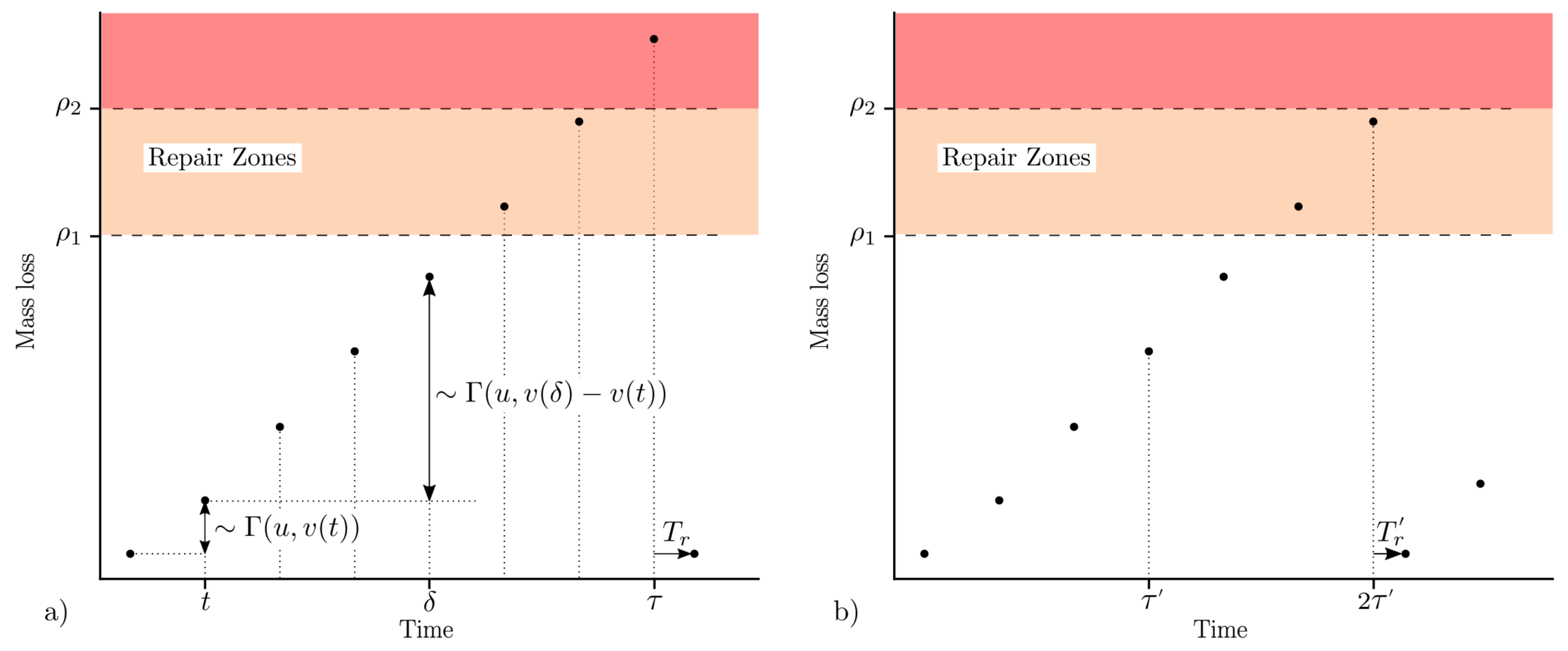
In this paper, we consider that the hydraulic runner has “failed” and needs to be repaired as soon its degradation level reaches a certain threshold. Beyond this degradation threshold, the component is still running, but its performance (i.e., efficiency) can be significantly altered.

In the following case study, we introduced two degradation thresholds representing moderate and severe erosion levels, denoted by ${\rho }_1$ and ${\rho }_2$ respectively, with ${\rho }_1<{\rho }_2$. It is considered that if the degradation level exceeds ${\rho }_2$, it is more likely that one or several blades might exhibit severe material erosion, such as perforation. In such a case, the repair process is more time-consuming and involves higher maintenance costs.

Inspections are performed at fixed time intervals and are noted $\tau$ with an associated cost $C_i$. For each inspection, the production unit is stopped for 1 day to perform an evaluation of material loss. Figure 1 represents the two previous degradation thresholds ${\rho }_1$ and ${\rho }_2$, along with $\tau$ for a given gamma process path.

After an inspection, 3 outcomes are possible:

• $X\left(\tau \right)<{\rho }_1$, the material is returned to production until a new inspection occurs.
• ${\rho }_1\le X\left(\tau \right)\le {\rho }_2$. The resulting degradation is considered as “moderate” and generates a repair operation with cost $C_r\left(t\right)$ and duration $T_r$. After a repair, the component is considered as good as new with $X(\tau +T_r)=0$.
• $X\left(\tau \right)\ge {\rho }_2$. The resulting degradation is considered as “severe” and generates a repair operation with cost $C_r\left(t\right)$. After a repair, the component is considered as good as new with $X(\tau +T_r^{\prime })=0$.

These 3 outcomes are presented in Figure 1. On the left, for the first inspection $t=\tau$, $X\left(t\right)$ is greater than ${\rho }_2$, which triggers a repair, resulting in $X(\tau +T_r)=0$. On the right, the first inspection $t={\tau }^{\prime }$ shows a degradation smaller than threshold ${\rho }_1$. Only on the next inspection $t=2{\tau }^{\prime }$ is a repair needed with $X\left(2{\tau }^{\prime }\right)\ge {\rho }_1$. For the remainder of this paper, S is the first time the component is repaired (as good as new) and $N_i$ is the number of inspections performed before the first repair (or during a repair cycle).

In this study, the following assumptions are deemed satisfied:

• the component remains in working order even if its degradation level exceeds threshold ${\rho }_2$,
• the repair cost $C_r(·)$ is a function only of the time $T_r$ needed to repair the component. $T_r$ is evaluated using the maintenance function $m(·)$,
• $m(·)$ depends on both the degradation level $X\left(t\right)$ and thresholds ${\rho }_1$ and ${\rho }_2$,
• during repair, the operating loss, denoted $C_{OL}\left(T_r\right)\ge 0$, is evaluated using $T_r$. $C_{OL}$ may vary depending on the electricity producer’s needs.

The maintenance efficiency, the function $m(·)$ is given in the following expression:

$$m\left(X\left(t\right)\right)=\left\{\begin{array}{cc}\hfill {\alpha }_{1}X\left(t\right)& \mathrm{if}{\rho }_1\le X\left(t\right)<{\rho }_2,\hfill \\ \hfill {\alpha }_{2}X\left(t\right)& \mathrm{if}X\left(t\right)\ge {\rho }_2,\hfill \end{array}\right.$$

(3)

with $0<{\alpha }_1<{\alpha }_2$. For a degradation level $X\left(t\right)\ge {\rho }_2$, we consider that the time to repair $T_r$ will be greater due to possible perforation of one or several blades requiring more complex repair operations. In Figure 1a, because a severe degradation (orange zone) is observed after an inspection, we have: $T_r^{\prime }>T_r$.

The total cost $C\left(S\right)$ of a repair cycle is given by the following expression:

$$C\left(S\right)=C_r\left(T_r\right)+N_i{C}_i+C_{OL}\left(T_r\right)$$

(4)

with $C_r\left(T_r\right)=\sigma T_r$ and $C_{OL}\left(T_r\right)=\beta T_r$ ($\sigma ,\beta \ge 0$).

As shown in Figure 1, we note that the process describing the component degradation in conjunction with the previous maintenance model, is a renewal process with renewal times being the dates of repair [12]. Indeed, after a repair occurs, the degradation state of components is equal to 0 and its evolution after the maintenance operation does not depend on its past. This renewal property allows us to use the so-called renewal theorems [13], which show that the expected cost of the component per unit of time is equal to the ratio of the expected cost incurred in a repair cycle divided by the expected length of a repair cycle:

$$\underset{t\to \infty }{lim}\frac{\mathbb{E}\left(C\right(t\left)\right)}{t}=\frac{\mathbb{E}\left(C\right(S\left)\right)}{\mathbb{E}\left(S\right)},$$

(5)

with $C(·)$ being the cumulative cost function and S the first repair (as good as new) date. This expression can be approximated using Equation (6):

$$\underset{t\to \infty }{lim}\frac{C\left(t\right)}{t}\sim R=\frac{\overline{C\left(S\right)}}{\overline{S}}$$

(6)

This result allows us to use a Monte Carlo simulation representing the degradation evolution to approximate with ratio R the expected cost of the component per time unit $[k\$/$day]. With a large enough number B of simulation replications, a convergence of Equation (6) is reached, allowing to compare different maintenance scenarios. The variability of $C\left(t\right)/t$ can be evaluated using the following equation:

$$V=var\left(C\left(S\right)-\frac{\overline{C\left(S\right)}S}{\overline{S}}\right)$$

(7)

4. Case Study

In this section, we study the influence of maintenance strategies on the component cost per unit of time over an infinite horizon. The main objective is to find a combination of both inspection intervals $\tau$ and maintenance thresholds ${\rho }_1$ minimizing the ratio R in Equation (6). To this end, we assume that cost parameters ${\alpha }_1,{\alpha }_2,\sigma ,C_i$ are fixed, except for those associated with operation losses $\beta$. Indeed, depending on the electricity producer’s needs (e.g., over a year), the unavailability of the component may have different financial impacts. To reflect these situations, 3 values of parameter $\beta$ are considered, as detailed in

Table 1. Simulation parameters.

Parameter		Comments
$\beta$	0	No operation loss
	50	Moderate operation losses
	100	High operation losses
${\alpha }_1$	0.20	${\rho }_1\le X\left(t\right)<{\rho }_2$
${\alpha }_2$	0.25	$X\left(t\right)\ge {\rho }_2$
$\sigma$	0.42	Repair cost per unit of time
$C_i$	0.42	Cost of inspection
${\rho }_1$	15	More conservative
	24	Moderately conservative
	33	Less conservative
${\rho }_2$	42	Perforation limit

. Parameters allowing to evaluate repair costs are summarized in the same table. Degradation level thresholds are presented in Table 1. Threshold ${\rho }_2=42$ kg represents a material loss level exhibiting a perforation. Thus, for a given threshold set $[{\rho }_1,{\rho }_2]$, only the first threshold ${\rho }_1$ may vary from one case to another. Note that degradation thresholds ${\rho }_1$ and ${\rho }_2$ are determined based on internal maintenance procedures and for a specific runner. Cavitation erosion is usually evaluated (during an inspection) by measuring the area and the depth of the affected regions [14]. In this case study, we considered that if material loss reaches 42 kg, it is more likely that the erosion depth will be equal to the blade thickness, resulting in perforation.

During operation, evaluating the cavitation intensity and the resulting erosion is a difficult task because this phenomenon is influenced by several operating conditions (suction head, head, discharge, etc.) [15]. For this purpose, different detection methods were developed and are used in industry [16] in conjunction with CFD models. For the sake of simplicity, the present case study considers a turbine subject to constant and steady operation conditions. To reflect various degradation conditions, 3 sets of gamma process parameters are proposed: from low to high degradation (with various dispersions) and are presented in

Table 2. Gamma process parameters with associated expectation and variance given at $t=12$ months.

GP Parameters $(\mathit{u},\mathit{c},\mathit{b})$	$\mathbb{E}$(X(12))	$\mathbb{V}$(X(12))	Comments
(1.29, 0.1, 1.13)	1.3	1	Low erosion
(5, 0.75, 1.13)	2.5	0.5	Moderate erosion
(4, 0.81, 1.2)	4	1	High erosion

. For a better physical understanding, the expectation and variance associated with previous sets of parameters are given at $t=12$ months. Moderate erosion parameters were obtained from a study conducted on a real Francis turbine in [17]. These data were collected from erosive cavitation monitoring system running over a 5-year span. Other parameters were derived to illustrate the methodology proposed in this paper.

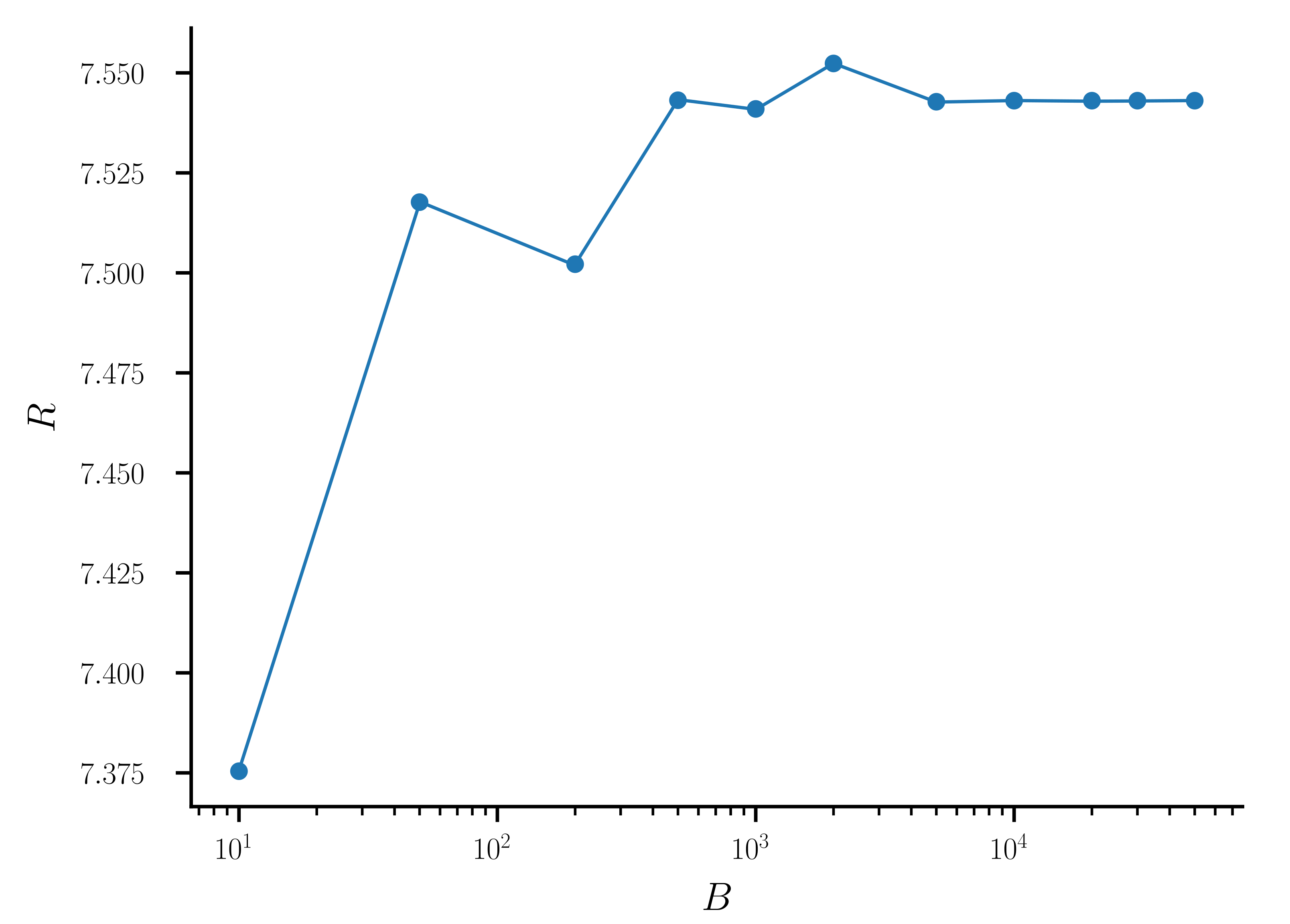
A convergence study on the ratio R and the associated variance V of simulated maintenance cycles was performed to determine the minimum number B of cycles needed to reach an asymptotic behaviour. The study showed that an asymptotic behaviour is reached for more than $B={8.10}^3$ cycles (see Figure 2). For the remainder of the case study, we generate $B={10}^4$ cycles.

5. Results

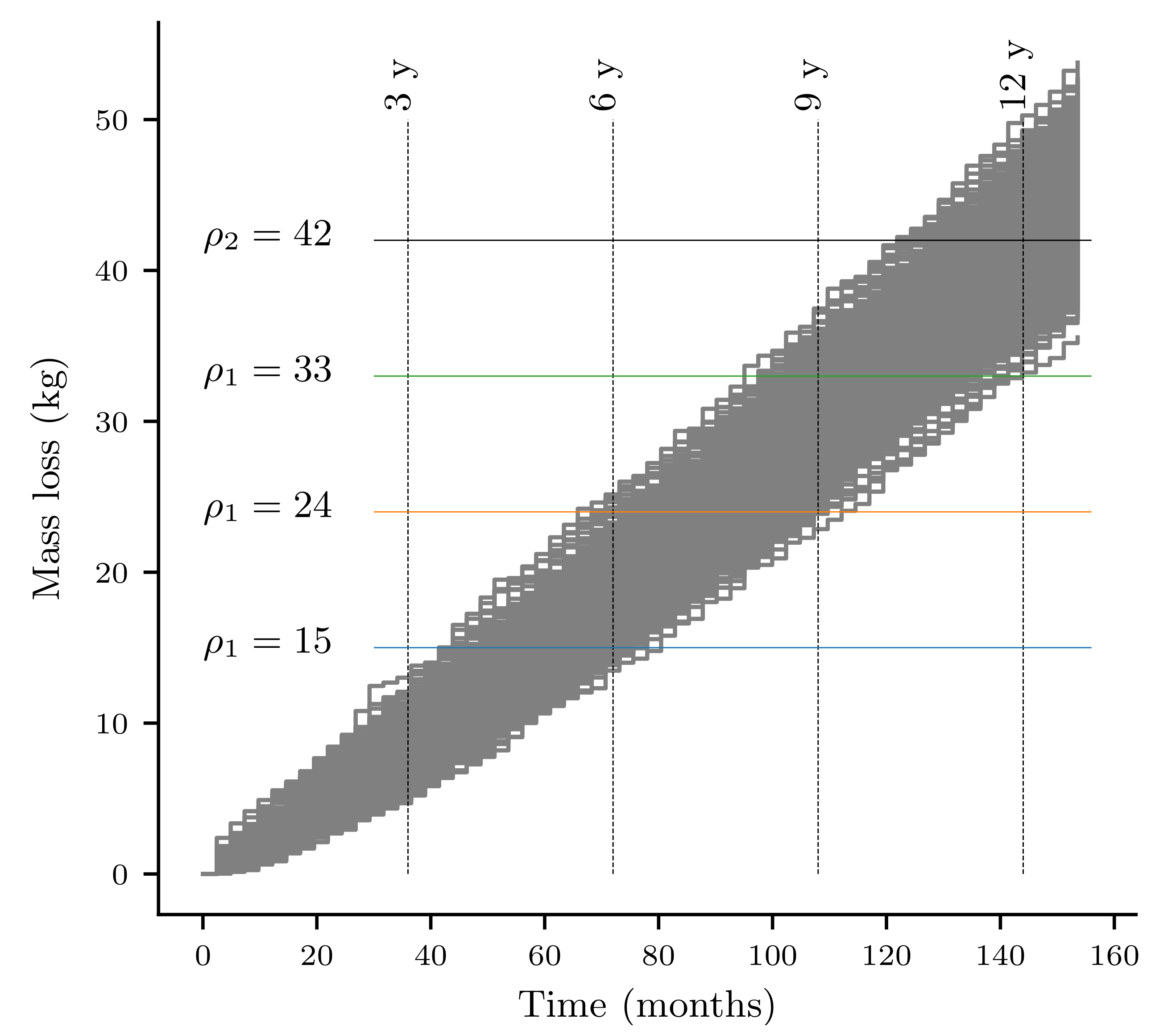
To facilitate the understanding of the results, Figure 3 shows a simulation of 1000 degradation paths over 14 years in the case of a moderate degradation. Note that maintenance operations are not considered in this figure. The different degradation thresholds are represented along with the four inspection intervals considered in this study. If we consider the inspection interval $\tau =6$ years, the first inspection generates mostly no repair operations for the cases where ${\rho }_1=24$ or 33 kg ($X\left(\tau \right)<{\rho }_1$). Conversely, for ${\rho }_1=$ 15 kg, most of the simulated paths show $X\left(\tau \right)\ge {\rho }_1$, generating a repair (after this repair, we observe a similar behaviour at $t=12$ years). Then, the next inspection occurs 6 years later at $t=12$ years. This time, for ${\rho }_1=24$ or 33 kg, we have about 50% of the degradation paths with $X\left(2\tau \right)\ge {\rho }_1$ and the rest with $X\left(2\tau \right)\ge {\rho }_2$. This observation explains the results shown in Figure 4 for GP parameters = $[5,0.75,1.13]$ and $\tau =6$ years: the case with ${\rho }_1=15$ kg shows the lower cost ratio R (at the first inspection, a repair is mandatory in most simulations). Similarly, for ${\rho }_1=22$ or 33 kg, R tends to be higher than for ${\rho }_1=15$ kg (two inspections are needed before a repair is performed). Also, because the degradation level $X(t=12$ years) is distributed around ${\rho }_2$, the dispersion of R will be higher for ${\rho }_1=23$ or 33 kg than for ${\rho }_1=15$ kg. The same logic applies for the results presented in Figure 4.

Figure 4 shows the influence of maintenance parameters on ratio R and its associated variance V. Note that while it is possible to have an approximation of the expected cost by unit of time with R for an infinite number of replications, we do not have a consistent approximation for confidence intervals. Hence, the variability is assessed using V to provide an idea of the dispersion of the results. In this graph, we considered $\beta =100$ to model operation losses due to turbine downtime. From left to right, we have different degradation intensities, ranging from moderate to severe. As expected, the most intense degradation exhibits the highest long-term cost per unit of time, expressed by ratio R. From the case study results, it appears that the degradation severity influences the optimal time interval $\tau$ between two inspections. For the low degradation, the larger time interval, $\tau =12$ years, gives the best results in terms of ratio R. Conversely, R is the lowest in the case $\tau =6$ years, for the moderate and most severe degradation. These results show that care should be taken in assessing the degradation intensity to determine the best time interval between inspections. For a low degradation, except for ${\rho }_1=24$ kg, the larger the value or $\tau$, the less the maintenance cost per unit of time. In every case presented, inspecting the system every 3 years does not represent an optimal choice.

For the three degradation intensities, the most conservative threshold set (with ${\rho }_1=15$ kg) shows the best results in terms of both ratio R and dispersion. Conversely, poorer results are observed for the highest value of ${\rho }_1$. In this case, being conservative on the degradation threshold and performing maintenance operations more often seems to represent the best repair strategy in terms of economics.

Results for other values of parameter $\beta$ are not presented in the figures as the overall behaviour observed is similar to the case of $\beta =100$. Although modelling operation losses may impact the values of R and V, that does not change the optimum or the results pattern, and thus, the same conclusions can be drawn.

6. Conclusions

In this paper, we studied the influence of inspection parameters on the long-term cost of operating a hydraulic runner subject to cavitation. To reflect the degradation variability phenomenon, a gamma process was used with different sets of parameters to represent various degradation severities.

For the case study presented, we showed that performing inspections at too close intervals ($\tau =3$ years) is never an optimal maintenance strategy. In our study, the best $\tau$ depends on the degradation severity. We showed that the most conservative degradation threshold exhibits the best results on both ratio R and its associated dispersion. The variance reflects how the cost to repair may vary for the same maintenance strategy. Different operation loss values did not impact the overall behaviour of maintenance strategies.

We highlight that from an industrial point of view, considering that only one cause of degradation or failure is not enough to represent the full complexity of the entire system considered in the study. The main objective of this paper was to propose a methodology that can be used in different contexts. A more intensive study should be conducted to incorporate the different causes of failure experienced with hydraulic turbines. Similarly, for the sake of simplicity, we considered only three levels of operation loss costs in the maintenance model. For more complete results, the analyst should put in extra effort to identify all costs associated with the maintenance operation and point out time of years exhibiting better conditions to perform a repair. Similarly, a drop in efficiency is expected when the turbine runner faces degradation [18]. On a practical level, for a highly accumulated degradation, the cost to operate the power unit is higher. This economic aspect should be incorporated in a future study to better reflect this reality. Even though loss of efficiency is difficult to track in practice, we believe that this should be accounted for in maintenance strategies.