A Concurrence Optimization Model for Low-Carbon Product Family Design and the Procurement Plan of Components under Uncertainty

Abstract

With the increase in pollution and people’s awareness of the environment, reducing greenhouse gas (GHG) emissions from products has attracted more and more attention. Companies and researchers are seeking appropriate methods to reduce the GHG emissions of products. Currently, product family design is widely used for meeting the diverse needs of customers. In order to reduce the GHG emission of products, some methods for low-carbon product family design have been presented in recent years. However, in the existing research, the related GHG emission data of a product family are given as crisp values, which cannot assess GHG emissions accurately. In addition, the procurement planning of components has not been fully concerned, and the supplier selection has only been considered. To this end, in this study, a concurrence optimization model was developed for the low-carbon product family design and the procurement plan of components under uncertainty. In the model, the relevant GHG emissions were considered as the uncertain number rather than the crisp value, and the uncertain GHG emissions model of the product family was established. Meanwhile, the order allocation of the supplier was considered as the decision variable in the model. To solve the uncertain optimization problem, a genetic algorithm was developed. Finally, a case study was performed to illustrate the effectiveness of the proposed approach. The results showed that the proposed model can help decision-makers to simultaneously determine the configuration of product variants, the procurement strategy of components, and the price strategies of product variants based on the objective of maximizing profit and minimizing GHG emission under uncertainty. Moreover, the concurrent optimization of low-carbon product family design and order allocation can bring the company greater profit and lower GHG emissions than just considering supplier selection in low-carbon product family design.

1. Introduction

Over the last few decades, greenhouse gas (GHG) emissions have attracted more and more attention. The Intergovernmental Panel on Climate Change indicates that human-made GHG emissions are the cause of global warming [1]. To reduce GHG emissions, many countries have issued relevant policies to encourage enterprises to design and manufacture low-carbon products, such as ISO 14064, PAS 2050, and ISO/TS 14067. Low-carbon product design has received more and more attention from academia and industry. To meet the various needs of customers, the product design method has changed from single product design to product family design. In recent years, some researchers have begun to study low-carbon product family design. For example, Wang et al. [2] presented an approach for modular product family design considering cost and GHG emissions. Xiao et al. [3] studied a method for collaborative optimization of product family design and manufacturing process planning. To focus on core competitiveness, more and more businesses choose to outsource the components to external suppliers. Since supplier selection affects both the production cost of the product and the GHG emissions of the product, Wang et al. [4] presented a method to simultaneously optimize supplier selection and the low-carbon design of the product family. Although some studies have discussed the low-carbon product family design, there are several shortcomings that need further research. First, the related GHG emissions data of the product family were considered as crisp values in the existing studies. However, in the realistic environment, some information is uncertain in the product family design stage, such as the mass of materials and the assembly process. Therefore, it is very difficult to accurately evaluate the GHG emissions of a product family from each stage. Second, it is meaningful that the product family design and the supply selection are considered simultaneously. Nevertheless, in previous studies, regardless of the number of requirements, one module instance of a product variant can only be provided by a single supplier. Yet, often, one module instance of a product variant can be provided by multiple suppliers. In other words, the order allocation of multiple suppliers has not been fully considered, and it will influence the low-carbon product family design. To make up for the above research gaps, this study proposes a concurrence optimization method for low-carbon product family design and the procurement decision of components under uncertainty. In the model, the relevant GHG emissions were considered as uncertain rather than as crisp values, and the uncertain GHG emissions model of the product family was established. Furthermore, instead of just considering the supplier selection, the order allocation of suppliers was considered as the decision variable in the model. Moreover, the genetic algorithm was developed for solving the uncertain optimization problem. The results showed that the decision model can assist managers/decision-makers to simultaneously determine the product family design and the procurement plan of components based on their goal preferences.

The structure of this article is as follows. Relevant existing studies, including low-carbon product design and product family design, are reviewed in Section 2. In Section 3, the problem is described. An optimization model is established in Section 4. Section 5 addresses the solution algorithm for solving the optimization model. To demonstrate the benefits of the proposed approach, a case study is provided in Section 6. Section 7 is the summary.

2. Literature Review

2.1. Low-Carbon Product Design

In recent years, low-carbon product design has attracted the attention of many scholars. Song et al. [5] developed a design auxiliary system using the bill of materials to design a low-carbon product. Qi et al. [6] integrated low-carbon technology into product modular design. Su et al. [7] proposed an approach to assess the carbon emissions and the cost in conceptual product design. According to the connection characteristics among components, Zhang et al. [8] approached the connection units with great carbon emissions. Kuo et al. [9] reported an optimization method for low-carbon product design considering cost, supplier capacity, and component transport. Xu et al. [10] built a low-carbon-product multi-objective optimization approach to deal with the contradictions among firms, consumers, and governments. He et al. [11] reported the low-carbon product design for the product life cycle. Chiang et al. [12] studied a method for developing a low-carbon electronic product. He et al. [13] proposed a conceptual framework for low-carbon product design. Zhang et al. [14] investigated a hybrid low-carbon optimization model for structural components considering material selection, structure layout, and structure parameters. The low-carbon product design method mentioned above is oriented to a single product. For meeting the diversified needs of customers, product family design with multiple product variants has been widely adopted in recent years. Since the design of product variants included in the product family are interrelated, the low-carbon design approach for a single product is not suitable for low-carbon product family design. To this end, some researchers began to study the low-carbon design method for product family. For example, Tang et al. [15] proposed an optimization model for low-carbon product configuration. Kim et al. [16] investigated an approach to identify a sustainable platform based on sustainability values, risk values, and commonality. Wang et al. [17] proposed a model to simultaneously optimize the low-carbon product family design and the remanufactured products.

Table 1. Some recent studies in low-carbon product design optimization models and our model.

Source	Model Description
	Object-Oriented		Objectives		Decision Variables			Uncertain GHG Emissions
	Single Product	Product Family	Single	Multiple	Product Configuration	Supplier Selection	Order Allocation
Kuo et al., 2014 [9]	√	--	--	Carbon footprints and cost	√	√	--	--
He et al., 2015 [11]	√	--	Carbon footprints	--	√	--	--	--
Chiang et al., 2015 [12]	√	--	GHG emissions	--	√	--	--	--
He et al., 2015 [13]	√	--	Carbon footprint	--	√	--	--	--
Wang et al., 2016 [2]	--	√	--	Cost and GHG emission	√	√	--	--
Tang et al., 2017 [15]	√	--	--	Profit and customer satisfaction	√	--	--	--
Wang et al., 2018 [4]	--	√	--	Profit and GHG emission	√	√	--	--
Wang et al., 2019 [17]	--	√	--	Profit and GHG emission	√	--	--	--
The proposed method of this research	--	√	--	Profit and GHG emission	√	√	√	√

shows some recent optimization models for low-carbon product design and our model. In the product family design stage, some information is uncertain, such as carbon emission factors, the mass of materials, and assembly process. As a result, it is very difficult to accurately evaluate the GHG emissions of the product family from each stage as crisp values. Therefore, the uncertain GHG emissions of the product family should be considered in low-carbon product family design, and it has not been concerned in the previous study.

2.2. Product Family Design

The product family design was considered a very useful way to enable mass customization because it can offer diversified products with a relatively low cost. In the past, many studies on product family design have been reported. Jiao et al. [18] presented a product family architecture for describing the logic mapping between functional, structural, and technical views of a product family. Du et al. [19] adopted a generic product structure to express hierarchical and structural organization of function modules, module instances, and product variants in a product family. Other studies focus on how to configure a product family from a set of alternative module instances. For instance, Oivares-Benitez et al. [20] used tabu search algorithms for selecting the product platform. Zacharias et al. [21] developed an optimal product family platform with consideration of engineering and marketing factors. Beyond that, many methods were proposed to address the measure of commonality in product platform design [22,23].

At present, supplier selection is very critical in manufacturing companies. The reasonable selection of suppliers cannot only reduce production costs but also enhance the competitiveness of products. There is no doubt that product family configuration and supplier selection are closely related. To this end, some scholars have optimized the product family design and supplier selection simultaneously. Huang et al. [24] addressed the problem of platform product decisions, manufacturing process decisions, and supply-sourcing decisions by adopting and extending the concept of the generic bills of materials of a product family. Huang et al. [25] adopted game-theoretic method to optimize the configuration of product family and supply chain design. In these studies, it is supposed that a product platform is predetermined. Luo et al. [26] investigated the concurrent optimization method of product family design and supplier selection in consideration of the choice behavior of a consumer. Cao et al. [27] presented a technique to optimize product family design and supplier selection under the multinomial logit consumer choice rule. Khalaf et al. [28] adopted a tabu search algorithm to configure product lines in consideration of time limits and assembly line constraints. With consideration of the quality and price, Rezapour et al. [29] presented a model for joint design of the product family and supply chain network. Luo et al. [30] studied the optimization of product family design with consideration of the supply risk and the discount. Yang et al. [31] investigated the joint design problem of the product family and the supply chain by adopting the leader–follower Stackelberg game method. From what has been discussed above, although the supplier selection and price decision of the product variant have been considered as decision variables in the low-carbon product family design, the procurement planning of components was not fully considered. Due to the fact that the order allocation of suppliers affects not only the profit of the product family but also the GHG emissions of the product family, the order allocation of suppliers should be considered as the decision variable in low-carbon product family design.

3. Problem Presentation

The optimization problem of this study is described as follows: a product is developed into a modular architecture, that is, a product can be considered to be composed of a group of function modules. For meeting the diverse needs of customers, the company plans to develop a product family that includes some product variants. Each function module of all product variants needs to be configured with module instances. In this study, it was supposed that module instances are provided by external suppliers and that the main company assembles the product. Several types of module instances can be supplied by a supplier, and multiple vendors can provide a module instance required by a product variant. In order to encourage business, different suppliers offer different discount schemes. The research problem of this study was how to simultaneously optimize the module instance configuration of all product variants included in the product family, the order allocation of suppliers, and the selling price of each product variant based on the objectives of maximizing profit and minimizing the GHG emissions of a product family.

The following basic assumptions were used in this research. (1) The total market can be divided into several market segments, and the purchase preferences of the customers in the same market segment were considered as the same [27]. (2) The candidate instances of each module had the same interface, and thus they can replace each other [27]. (3) The unqualified suppliers were excluded, and all candidate suppliers were qualified [4]. (4) A supplier can provide several different module instances [4]. (5) One module instance of a product variant can be provided by multiple suppliers. (6) All candidate suppliers can deliver on time, and the supplying capacity of candidate suppliers meets the requirements [4].

To formulate the optimization model, the following notations were defined:

(1)

Indices

m: (m = 1, 2, …, M) index for modules

n: (n = 1, 2, …, N) index for module instance

M_m,n: nth instance of mth module

t: (t = 1, 2, …, T) index for product variant

z: (z = 1, 2, …, Z) index for supplier

a: (a = 1, 2, …, A) index for market segment

(2)

Parameters

$U_{pro}^{t(a)}$: the utility of the tth product variant in the ath market segment

${\mu }_{mn}^{(a)}$: the utility of module instance M_m,n in the ath market segment

${\lambda }^{t(a)}$: the surplus utility of tth product variant in the ath market segment

$\delta$: the scaling parameter in the MNL rule

E: the number of similar products launched by other companies

λ^e(a): the surplus utility of eth similar product in the ath market segment

$Q_t^{(a)}$: the possible demand of tth product variant in the ath market segment

n_q: the total product demand in the ath market segment

R_T: the expected revenue

C: total cost

$C^{\mathrm{in}}$: production cost within the enterprise

$C^{\mathrm{out}}$: external procurement cost

$C^{\mathrm{in}\left(\mathrm{fix}\right)}$: fixed production cost within the enterprise

$C^{\mathrm{in}\left(\mathrm{var}\right)}$: variable production cost within the enterprise

$c_{mn}^{\mathrm{in}\left(\mathrm{var}\right)}$: unit variable production cost of module instance M_m,n

$C^{\mathrm{out}\left(\mathrm{fix}\right)}$: fix cost of using suppliers

$C^{\mathrm{out}\left(\mathrm{var}\right)}$: variant cost from procurement

E_z: fixed cost of selection the zth supplier

G_z: binary variable such that G_z = 1 if the zth supplier is selected, and G_z = 0 otherwise

$p_{mn}^z$: purchase price of M_m,n provided by the zth supplier

${\delta }_z$: discount rate provided by the zth supplier

$m_{mn}^z$: the weight of M_m,n provided by the zth supplier

S_z: distance from the zth supplier to the assembly firm

$C_{Tr}$: unit transportation cost

E^T: total greenhouse gas (GHG) emissions

$E_{com}^T$: GHG emission from component

$E_{tra}^T$: GHG emission from transportation

$E_{pro}^T$: GHG emission from production within the assembly firm

$E_{\sup }^{sel}$: GHG emission from supplier selection

$g_{mn}^z$: Order poportion of zth supplier to supply module instance M_m,n.

(3)

Decision variables

$$y_{mn}^{(t)}=\{\begin{array}{l}1\hspace{1em}\hspace{1em}\mathrm{if} n\mathrm{th} \mathrm{instance} \mathrm{of} m\mathrm{th} \mathrm{module} ({\mathrm{M}}_{m,n}) \mathrm{is} \mathrm{used} \mathrm{to} \mathrm{configure} \mathrm{to} \mathrm{the} t\mathrm{th} \mathrm{product} \mathrm{variant}\\ \hspace{1em}\hspace{1em}(m=1, 2, \dots , M; n=1, 2, \dots , N; t=1, 2, \dots , T)\\ 0\hspace{1em}\hspace{1em}\mathrm{otherwise}\end{array}$$

(1)

$$N_{mn}^z: \mathrm{the} \mathrm{purchase} \mathrm{amount} \mathrm{of} n\mathrm{th} \mathrm{instance} \mathrm{of} m\mathrm{th} \mathrm{module} ({\mathrm{M}}_{i,j}) \mathrm{from} z\mathrm{th} \mathrm{supplier}$$

(2)

$$p_t: \mathrm{the} \mathrm{price} \mathrm{of} t\mathrm{th} \mathrm{product} \mathrm{variant} (t=1, 2, \dots , T)$$

(3)

4. Establishment of the Optimization Model

4.1. Establishing Customer Preference Model

To establish the customer preference model, the product market was divided into several segments in advance. Clustering technology can be used to complete market segmentation [32]. Moreover, it is necessary to estimate the size of each market segment.

In previous studies, the utility function has been widely used to measure customer preference. The customer preference model was established based on the utility function. In light of the part-worth model [33], the utility of the tth product variant in the ath market segment, $U_{pro}^{t(a)}$, was calculated as follows:

$$U_{pro}^{t(a)}={\displaystyle \sum _{m=1}^M{\displaystyle \sum _{n=1}^N{y}_{{}_{mn}}^{(t)}}}{\mu }_{mn}^{(a)}+{\eta }_r$$

(4)

where ${\mu }_{mn}^{(a)}$ is the utility of module instance M_m,n in the ath market segment, and it can be estimated by conjoint analysis; ${\eta }_r$ is a constant.

When customers buy products, they should consider the selling price of a product as well as the utility. Considering the selling price of product, the surplus utility of tth product variant in the ath market segment (${\lambda }^{t(a)}$) is evaluated as:

$${\lambda }^{t(a)}=U_{pro}^{t(a)}-p_t$$

(5)

where p_t is the the selling price of tth product variant.

4.2. Market Demand of Products and Expected Revenue

Generally, customers’ decisions to buy a product is not only affected by the surplus utility of the product but also by other similar products. For this reason, the probabilistic choice rule was adopted in many studies to represent customers’ decisions for purchases. The probabilistic choice rule supposes that utility is a random variable and that customers choose products based on the criterion of random utility maximization. In the probabilistic choice rule, the multinomial logit choice (MNL) rule was adopted in this research due to its simplicity. According to the MNL rule, the probability of the tth product variant being selected in the ath market segment is calculated as follows:

$$P_t^{(a)}=\frac{e^{\delta {\lambda }^{t(a)}}}{{\displaystyle \sum _{t=1}^T{e}^{\delta {\lambda }_{}^{t(a)}}}+{\displaystyle \sum _{e=1}^E{e}^{\delta {\lambda }_{}^{e(a)}}}}$$

(6)

where $\delta$ in the MNL rule is the scaling parameter and E represents the number of similar products launched by other companies. ${\lambda }_{}^{e(a)}$ is the surplus utility of eth similar product in the ath market segment.

The possible demand of tth product variant in the ath market segment ($Q_t^{(a)}$) is expressed as follows:

$$Q_t^{(a)}=n_q{P}_t^{(a)}$$

(7)

where n_q is total the product requirement in the ath market segment.

When the market demand and the price of each product variant included in the product family are known, the expected revenue (R_T) can be estimated as follows:

$$R_T={\displaystyle \sum _{a=1}^A{\displaystyle \sum _{t=1}^T{Q}_t^{(a)}{p}_t}}$$

(8)

4.3. Price Discount of Suppliers

Generally, a company procures components from multiple suppliers rather than a single supplier. To get a large order, suppliers may offer price discounts. The volume discount based on order income is widely used by suppliers, and it was considered in this research.

Table 2. An example of discount.

Sales Volume (USD)	Discount (%)
[0, 20,000)	0
[20,000, 80,000)	5
Equal to or more than 80,000	10

shows an example of a discount. For instance, there was no discount when the purchase value was less than USD 20,000. When the total purchase value was in the range of USD 20,000 to USD 80,000, the buyer can enjoy a 5% discount of the total purchase value.

4.4. Production Cost of a Product Family

The total cost can be divided into the production cost within the enterprise ($C^{\mathrm{in}}$) and the external procurement cost ($C^{\mathrm{out}}$), and the total cost C is formulated as:

$$C=C^{\mathrm{in}}+C^{\mathrm{out}}$$

(9)

$C^{\mathrm{in}}$ is the production cost within the enterprise, and it consists of two parts. The two parts are the fixed cost ($C^{\mathrm{in}\left(\mathrm{fix}\right)}$) and the variable cost ($C^{\mathrm{in}\left(\mathrm{var}\right)}$). $C^{\mathrm{in}\left(\mathrm{fix}\right)}$ includes the development cost, the management cost, etc. $C^{\mathrm{in}\left(\mathrm{var}\right)}$ indicates the product assembly cost, the product packaging cost, etc.

The number of product variants (v) developed in a product family affects the $C^{\mathrm{in}\left(\mathrm{fix}\right)}$, and $C^{\mathrm{in}\left(\mathrm{fix}\right)}$ is expressed as follows:

$$C^{\mathrm{in}\left(\mathrm{fix}\right)}=\{\begin{array}{l}{Y}_1\hspace{1em}\hspace{1em}\hspace{1em}v=1\\ Y_2\hspace{1em}\hspace{1em}\hspace{1em}v=2\\ ⋮\\ Y_v\hspace{1em}\hspace{1em}\hspace{1em}v=V\end{array}$$

(10)

where Y_v represent the fixed cost, and it corresponds to the number of product variants.

The $C^{\mathrm{in}\left(\mathrm{var}\right)}$ can be expressed as:

$$C^{\mathrm{in}\left(\mathrm{var}\right)}={\displaystyle \sum _{a=1}^A{\displaystyle \sum _{t=1}^T{\displaystyle \sum _{m=1}^M{\displaystyle \sum _{n=1}^N{Q}_t^{(a)}{c}_{mn}^{\mathrm{in}\left(\mathrm{var}\right)}{y}_{mn}^{(t)}}}}}$$

(11)

where $c_{mn}^{\mathrm{in}\left(\mathrm{var}\right)}$ is the unit variable production cost of module instance M_m,n.

Based on Equations (10) and (11), $C^{\mathrm{in}}$ is reformulated as follows:

$$C^{\mathrm{in}}=Y_v+{\displaystyle \sum _{a=1}^A{\displaystyle \sum _{t=1}^T{\displaystyle \sum _{m=1}^M{\displaystyle \sum _{n=1}^N{Q}_t^{(a)}{c}_{mn}^{\mathrm{in}\left(\mathrm{var}\right)}{y}_{mn}^{(t)}}}}}$$

(12)

$C^{\mathrm{out}}$ is also divided into two parts, including the fixed cost of using suppliers ($C^{\mathrm{out}\left(\mathrm{fix}\right)}$) and the variant cost ($C^{\mathrm{out}\left(\mathrm{var}\right)}$).

$C^{\mathrm{out}\left(\mathrm{fix}\right)}$ is related to the adopted suppliers, such as the negotiation cost and so on. $C^{\mathrm{out}\left(\mathrm{fix}\right)}$ is expressed as:

$$C^{\mathrm{out}(fix)}={\displaystyle \sum _{z=1}^Z{E}_z{G}_z}$$

(13)

where E_z represents the fixed cost of selection of the zth supplier; the value of G_z is 1 when the zth supplier is selected, and, if not selected, the value of G_z is 0.

$C^{\mathrm{out}\left(\mathrm{var}\right)}$ indicates the purchasing cost of module instances and the transportation cost. $C^{\mathrm{out}\left(\mathrm{var}\right)}$ can be formulated as follows:

$$C^{\mathrm{out}\left(\mathrm{var}\right)}={\displaystyle \sum _{z=1}^Z\left[{\displaystyle \sum _{m=1}^M{\displaystyle \sum _{n=1}^N{\displaystyle \sum _{a=1}^A{\displaystyle \sum _{t=1}^T{Q}_t^{(a)}{y}_{mn}^{(t)}{N}_{mn}^z{p}_{mn}^z}}}}\right]}(1-{\delta }_z)+{\displaystyle \sum _{z=1}^Z\left[{\displaystyle \sum _{m=1}^M{\displaystyle \sum _{n=1}^N{\displaystyle \sum _{a=1}^A{\displaystyle \sum _{t=1}^T{Q}_t^{(a)}{y}_{mn}^{(t)}{N}_{imn}^z{m}_{mn}^z}}}}\right]}{S}^z{C}_{Tr}$$

(14)

where $p_{mn}^z$ represents the purchase price of M_m,n provided by the zth supplier; ${\delta }_z$ is the discount rate, which can be provided by the zth supplier; $m_{mn}^z$ indicates the weight of M_m,n provided by the zth supplier; S_z represents the distance from the zth supplier to the assembly firm; C_Tr represents the unit transportation cost.

By combining Equations (13) and (14), $C^{\mathrm{pur}}$ is reformulated as:

$$C^{\mathrm{out}}={\displaystyle \sum _{z=1}^Z{E}_z{G}_z}+{\displaystyle \sum _{z=1}^Z\left[{\displaystyle \sum _{m=1}^M{\displaystyle \sum _{n=1}^N{\displaystyle \sum _{a=1}^A{\displaystyle \sum _{t=1}^T{Q}_t^{(a)}{y}_{mn}^{(t)}{N}_{mn}^z{p}_{mn}^z}}}}\right]}(1-{\delta }_z)+{\displaystyle \sum _{z=1}^Z\left[{\displaystyle \sum _{m=1}^M{\displaystyle \sum _{n=1}^N{\displaystyle \sum _{a=1}^A{\displaystyle \sum _{t=1}^T{Q}_t^{(a)}{y}_{mn}^{(t)}{N}_{mn}^z{m}_{mn}^z}}}}\right]}{S}^z{C}_{Tr}$$

(15)

4.5. Greenhouse Gas Emission Model of a Product Family

The total greenhouse gas emission (GHG) emissions, E^T, was divided into four parts. The four parts were GHG emissions from the component ($E_{com}^T$), GHG emissions from transportation ($E_{tra}^T$), GHG emissions from production within the enterprise ($E_{pro}^T$), and GHG emissions from the supplier selection ($E_{\sup }^{sel}$). E^T is expressed as:

$$E^T=E_{com}^T+E_{tra}^T+E_{pro}^T+E_{\sup }^{sel}$$

(16)

$E_{com}^T$ is formulated as follows:

$$E_{com}^T={\displaystyle \sum _{m=1}^M{\displaystyle \sum _{n=1}^N{\displaystyle \sum _{a=1}^A{\displaystyle \sum _{t=1}^T{Q}_t^{(a)}{y}_{mn}^{(t)}[e_{mn}^{z-L},}}}}{e}_{mn}^{z-R}]$$

(17)

where $[e_{mn}^{z-L},e_{mn}^{z-R}]$ is an interval number, and it is the possible GHG emission for the module instance M_m,n provided by zth supplier.

The total GHG emissions from transportation of the module instance, $E_{tra}^T$, can be described as follows:

$$E_{tra}^T={\displaystyle \sum _{z=1}^Z\sum _{m=1}^M{\displaystyle \sum _{n=1}^N{\displaystyle \sum _{a=1}^A{\displaystyle \sum _{t=1}^T{Q}_t^{(a)}{y}_{mn}^{(t)}{N}_{mn}^z{m}_{mn}^z{S}^z[}}}}{E}_{Tr}^L,E_{Tr}^R]$$

(18)

where $[E_{Tr}^L,E_{Tr}^R]$ is an interval number, and it indicates the possible unit transportation GHG emissions.

$E_{pro}^T$, including the fixed part $[E_{pro}^{fix(V)-L},E_{pro}^{fix(V)-R}]$ and the variable part $E_{pro}^{\mathrm{var}}$, is the GHG emissions from production within the enterprise. $[E_{pro}^{fix(V)-L},E_{pro}^{fix(V)-R}]$ is an interval number, and it represents the possible fixed GHG emissions of the product family with development V product variants, and this part is mainly from product development, management, etc. $E_{pro}^{\mathrm{var}}$ is mainly from product assembly, packing of products, etc. and can be formulated as:

$$E_{pro}^{\mathrm{var}}={\displaystyle \sum _{a=1}^A{\displaystyle \sum _{t=1}^T{\displaystyle \sum _{m=1}^M{\displaystyle \sum _{n=1}^N{Q}_t^{(a)}{y}_{mn}^{(t)}[}}}}{e}_{mn}^{\left(\mathrm{ass}\right)-\mathrm{L}},e_{mn}^{\left(\mathrm{ass}\right)-\mathrm{R}}]$$

(19)

where $[e_{mn}^{\left(\mathrm{ass}\right)-\mathrm{L}},e_{mn}^{\left(\mathrm{ass}\right)-\mathrm{R}}]$ is an interval number, representing the possible GHG emissions of assembly for M_m,n.

$E_{pro}^T$ can be reformulated as follows:

$$E_{pro}^T=[E_{pro}^{fix(V)-L},E_{pro}^{fix(V)-R}]+{\displaystyle \sum _{a=1}^A{\displaystyle \sum _{t=1}^T{\displaystyle \sum _{m=1}^M{\displaystyle \sum _{n=1}^N{Q}_t^{(a)}{y}_{mn}^{(t)}[}}}}{e}_{mn}^{\left(\mathrm{ass}\right)-\mathrm{L}},e_{mn}^{\left(\mathrm{ass}\right)-\mathrm{R}}]$$

(20)

$E_{\sup }^{sel}$ is mainly from negotiation communication, relationship maintenance between company and suppliers, etc. It can be formulated as follows:

$$E_{\sup }^{sel}={\displaystyle \sum _{z=1}^Z[F_Z^L,F_Z^R]G_z}$$

(21)

where $[F_Z^L,F_Z^R]$ represents the possible GHG emission when the zth supplier is adopted.

4.6. Objective Function of the Optimization Model

Profit maximization is the first considered by enterprises, and the first optimization objective f₁ can be expressed as:

$$f_1=\max \mathsf{\Delta }=T_{rev}-C$$

(22)

Based on Equations (8), (12) and (15), f₁ is rewritten as follows:

$$\begin{array}{l}{f}_1=\max \mathsf{\Delta }=\max {\displaystyle \sum _{a=1}^A{\displaystyle \sum _{t=1}^T{Q}_t^{(a)}{p}_t}}-Y_v-{\displaystyle \sum _{a=1}^A{\displaystyle \sum _{t=1}^T{\displaystyle \sum _{m=1}^M{\displaystyle \sum _{n=1}^N{Q}_t^{(a)}{c}_{mn}^{\mathrm{in}\left(\mathrm{var}\right)}{y}_{mn}^{(t)}-{\displaystyle \sum _{z=1}^Z{E}_z{G}_z}}}}}\\ -{\displaystyle \sum _{z=1}^Z\left[{\displaystyle \sum _{m=1}^M{\displaystyle \sum _{n=1}^N{\displaystyle \sum _{a=1}^A{\displaystyle \sum _{t=1}^T{Q}_t^{(a)}{y}_{mn}^{(t)}{N}_{mn}^z{p}_{mn}^z}}}}\right]}(1-{\delta }_z)-{\displaystyle \sum _{z=1}^Z\left[{\displaystyle \sum _{m=1}^M{\displaystyle \sum _{n=1}^N{\displaystyle \sum _{a=1}^A{\displaystyle \sum _{t=1}^T{Q}_t^{(a)}{y}_{mn}^{(t)}{N}_{mn}^z{m}_{mn}^z}}}}\right]}{S}^z{C}_{Tr}\end{array}$$

(23)

Minimizing GHG emissions, f₂ is another optimization goal in low-carbon product family design. f₂ is expressed as follows:

$$f_2=\min E^T$$

(24)

According to Equations (17), (18), (20) and (21), f₂ is formulated as follows:

$$\begin{array}{l}{f}_2=\min (E^T)=\min {\displaystyle \sum _{m=1}^M{\displaystyle \sum _{n=1}^N{\displaystyle \sum _{a=1}^A{\displaystyle \sum _{t=1}^T{Q}_t^{(a)}{y}_{mn}^{(t)}[e_{mn}^{z-L},}}}}{e}_{mn}^{z-R}]+{\displaystyle \sum _{z=1}^Z{\displaystyle \sum _{m=1}^M{\displaystyle \sum _{n=1}^N{\displaystyle \sum _{a=1}^A{\displaystyle \sum _{t=1}^T{Q}_t^{(a)}{y}_{mn}^{(t)}{N}_{mn}^z{m}_{mn}^z}}}}}{S}^z[E_{Tr}^L,E_{Tr}^R]\\ +[E_{pro}^{fix(V)-L},E_{pro}^{fix(V)-R}]+{\displaystyle \sum _{a=1}^A{\displaystyle \sum _{t=1}^T{\displaystyle \sum _{m=1}^M{\displaystyle \sum _{n=1}^N{Q}_t^{(a)}[e_{mn}^{\left(\mathrm{ass}\right)-\mathrm{L}},e_{mn}^{\left(\mathrm{ass}\right)-\mathrm{R}}]y_{mn}^{(t)}}}}}+{\displaystyle \sum _{z=1}^Z[F_z^L,F_z^R]G_z}\end{array}$$

(25)

4.7. Optimization Constraints

(1)

Selective constraint in product variant configuration

Although there are several candidate module instances for each function module, only one instance can be selected for each function module of each product variant. It can be formulated as follows:

$${\displaystyle \sum _{n=1}^N{y}_{mn}^{(t)}}=1, (t=1, 2, \dots , T; m=1, 2, \dots , M)$$

(26)

(2)

Order quantity constraint of the module instance

For a module instance, it can be provided by one supplier or several suppliers. The total amount of module instances provided by all suppliers is equal to the number of requirements, and it can be described as follows:

$${\displaystyle \sum _{a=1}^A{\displaystyle \sum _{t=1}^T(Q_t^{(a)}{y}_{mn}^{(t)})={\displaystyle \sum _{z=1}^Z{N}_{mn}^z}}} (m=1, 2, \dots \dots , M; n=1, 2, \dots \dots , N)$$

(27)

(3)

Minimum order quantity

If supplier z is selected to provide M_m,n, the purchase amount from supplier z cannot be less than $M{N}_{i,j}^z$.

$$N_{mn}^z \ge M{N}_{mn}^z (z=1, 2, \dots \dots , Z; m=1, 2, \dots \dots , M; n=1, 2\dots \dots , N)$$

(28)

(4)

Configuration constraint.

The configuration of any two product variants cannot be exactly the same.

4.8. Treatment of the Uncertain Objective Function (f₂)

The optimization goal, f₂, of the proposed model contains an interval number, and it is treated in this section.

In interval mathematics, an uncertain objective function f can be transformed into the following double-goals optimization problem [34]:

$$m(f(\tilde{x},B_{}))=\frac{1}{2}(f_{}^L(\tilde{x},B_{})+f_{}^R(\tilde{x},B_{}))$$

(29)

$$w(f_{}(\tilde{x},B_{}))=\frac{1}{2}(f_{}^L(\tilde{x},B_{})-f_{}^R(\tilde{x},B_{}))$$

(30)

where m is called the midpoint value, w is called the radius of the interval number, B is the uncertain vector, and its components are all interval numbers, $B=\left\{b^L\le b\le b^R\right\}$.

In Equations (29) and (30), $f_{}^L$ and $f_{}^R$ are calculated as follows [35]:

$$f_{}^L(\tilde{x},B_{})=\underset{C\in \mathsf{\Gamma }}{\min }{f}_{}^{}(\tilde{x},B_{}),f_{}^R(\tilde{x},B_{})=\underset{C\in \mathsf{\Gamma }}{\max }{f}_{}^{}(\tilde{x},B_{})$$

(31)

This study adopted the linear combination approach to deal with two objective functions: $f_{}^L$ and $f_{}^R$. Adopting this approach to integrate $f_{}^L$ and $f_{}^R$ is relatively easy, given that the preference of the objective function is available. It is expressed as:

$$\begin{array}{l}{f}_{}=d_{1}m(f_{}(\tilde{x},C_{}))+d_{2}w(f_{}(\tilde{x},C_{})),\\ d_1,d_2\ge 0, d_1+d_2=1\end{array}$$

(32)

According to the approach mentioned above, in this study, the uncertain objective function f₂ of the proposed model can be treated as:

$$f_2=\min (E^T)=\min (d_{1}m(E^T)+d_{2}w(E^T))$$

(33)

where d₁ is the weight for m(E^T), d₂ is the weight for w(E^T), and m(E^T) and w(E^T) are formulated as follows:

$$\begin{array}{l}\mathrm{m}(E^T)={\displaystyle \sum _{m=1}^M{\displaystyle \sum _{n=1}^N{\displaystyle \sum _{a=1}^A{\displaystyle \sum _{t=1}^T{Q}_t^{(a)}{y}_{mn}^{(t)}\times \frac{1}{2}(e_{mn}^{z-L}+}}}}{e}_{mn}^{z-R})+{\displaystyle \sum _{z=1}^Z{\displaystyle \sum _{m=1}^M{\displaystyle \sum _{n=1}^N{\displaystyle \sum _{a=1}^A{\displaystyle \sum _{t=1}^T{Q}_t^{(a)}{y}_{mn}^{(t)}{N}_{mn}^z{m}_{mn}^z}}}}}{S}^z\times \frac{1}{2}(E_{Tr}^L+E_{Tr}^R)\\ +\frac{1}{2}(E_{pro}^{fix(V)-L}+E_{pro}^{fix(V)-R})+{\displaystyle \sum _{a=1}^A{\displaystyle \sum _{t=1}^T{\displaystyle \sum _{m=1}^M{\displaystyle \sum _{n=1}^N{Q}_t^{(a)}\times \frac{1}{2}(e_{mn}^{\left(\mathrm{ass}\right)-\mathrm{L}}+e_{mn}^{\left(\mathrm{ass}\right)-\mathrm{R}})y_{mn}^{(t)}}}}}+{\displaystyle \sum _{z=1}^Z\frac{1}{2}(F_z^L+F_z^R)G_z}\end{array}$$

(34)

$$\begin{array}{l}w(E^T)={\displaystyle \sum _{m=1}^M{\displaystyle \sum _{n=1}^N{\displaystyle \sum _{a=1}^A{\displaystyle \sum _{t=1}^T{Q}_t^{(a)}{y}_{mn}^{(t)}\times \frac{1}{2}(e_{mn}^{z-R}-}}}}{e}_{mn}^{z-L})+{\displaystyle \sum _{z=1}^Z{\displaystyle \sum _{m=1}^M{\displaystyle \sum _{n=1}^N{\displaystyle \sum _{a=1}^A{\displaystyle \sum _{t=1}^T{Q}_t^{(a)}{y}_{mn}^{(t)}{N}_{mn}^z{m}_{mn}^z}}}}}{S}^z\times \frac{1}{2}(E_{Tr}^R-E_{Tr}^L)\\ +\frac{1}{2}(E_{pro}^{fix(V)-R}-E_{pro}^{fix(V)-L})+{\displaystyle \sum _{a=1}^A{\displaystyle \sum _{t=1}^T{\displaystyle \sum _{m=1}^M{\displaystyle \sum _{n=1}^N{Q}_t^{(a)}\times \frac{1}{2}(e_{mn}^{\left(\mathrm{ass}\right)-\mathrm{R}}-e_{mn}^{\left(\mathrm{ass}\right)-\mathrm{L}})y_{mn}^{(t)}}}}}+{\displaystyle \sum _{z=1}^Z\frac{1}{2}(F_z^R-F_z^L)G_z}\end{array}$$

(35)

4.9. Optimization Model Representation

According to the above analysis, the problem is a constrained bi-objective programming problem, and it is shown as follows:

$$\begin{array}{l}\mathrm{objective}:\{\begin{array}{l}{f}_1: \mathrm{Equation} (25)\\ f_2: \mathrm{Equation} (33)\end{array}\\ s.t.\{\begin{array}{l}\mathrm{Equations} (26)–(28)\\ Configuration constraint\\ \mathrm{Equations} (3)–(5)\\ y_{ij}^{(r)} \in \left\{0,1\right\} , N_{ij}^z \ge 0, \mathrm{and} p_r>0\end{array}\end{array}$$

(36)

5. Solving the Optimization Model Using Genetic Algorithm (GA)

The proposed optimization model is a combinatorial optimization problem and, thus, is an NP-hard one. As a consequence, it is very difficult to be solved by classical mathematical programming methods, especially considering the large-sized problem. The meta-heuristic algorithm is more effective than the traditional methods. Many heuristic algorithms have been proposed to solve the combinatorial optimization problem. Due to its simple calculation and robust search ability, the genetic algorithm was employed in this study.

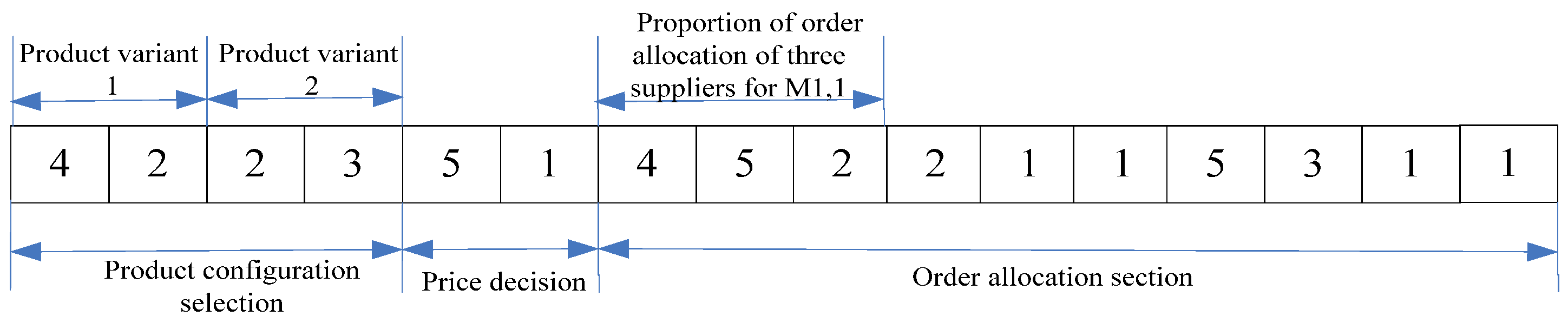
5.1. Chromosome of GA

The essential part of GA implementation is the representation of the problem to be solved with a finite-length string called a chromosome. Every chromosome in the population represents one solution for the problem. This study adopted the integer-coding method, and the chromosome was a 1-dimensional array with multiple cells. Each cell is called a gene. Figure 1 shows the chromosome structure used in this research. A chromosome was divided into three sections, including the product variant configuration section, the price decision section, and the order allocation section. The three sections were further divided into several sub-sections. As shown in Figure 1, the chromosome contained two sub-sections in the product configuration section. It means that two product variants need to be developed in the product family. Each sub-section has three genes, which means that the module instances need to be configured for the three function modules of each product variant. The numerical value in the gene indicates which module instance is selected. For example, the numerical value was “3” in the fourth gene, and it represents that the module instance M_2,3 was selected to configure the second module of product variant 2. In this research, the price was discretized, and the discrete prices were coded in advance. The price selected for each product variant was indicated by the gene value in the price selection section. For instance, the numerical value was “5” in the first gene of the price decision section, and it means that the fifth discrete price was selected for product variant 1. In the order allocation section, it represents the proportion of the order allocation. The numerical value in the gene was an integer value varying from 1 to 9. For example, as shown in Figure 1, three suppliers (S1, S2, and S3) can supply the module instance M_1,1, and the proportion of order allocation was 4:5:2, which is indicated by the numerical value in the gene. Therefore, when the total demand of the module instance M_1,1 was known, the order volume allocated for three suppliers can be calculated. Assuming that there are $Z^{\prime }$ suppliers who can provide module instance M_i,j, the order volume allocated to the zth supplier ($N_{ij}^z$) is computed as follows:

$$N_{mn}^z=\frac{{\displaystyle \sum _{t=1}^T{\displaystyle \sum _{a=1}^A{Q}_t^{(a)}{y}_{mn}^t}}}{{\displaystyle \sum _{z=1}^{Z^{\prime }}{g}_{mn}^z}}{g}_{mn}^z (m=1, 2, \dots , M; n=1, 2, \dots , N; z=1, 2, \dots , Z)$$

(37)

where $g_{mn}^z$ is the order proportion of the zth supplier to supply module instance M_m,n.

5.2. Fitness Function

For solving the proposed bi-objective optimization problem, this study adopted the weighting approach to integrate the two optimization objectives. The weights u₁ and u₂ $(u_1+u_2=1,u_1\ge 0,u_2\ge 0)$ were assigned for the two optimization objectives. u₁ was allocated for profit (f₁), and u₂ was allocated for GHG emissions (f₂). The order of magnitude of the profit and GHG emissions may be different; therefore, f₁ and f₂ need to be normalized. The normalized objectives with weights were formulated as follows:

$$F^{\prime }(k)=u_1{f_1}^{\prime }(k)+u_2{f}_2^{\prime }(k)$$

(38)

where ${f_i}^{\prime }$ is the normalized values and was obtained as follows:

$${f_i}^{\prime }(k)=\frac{f_i(k)-f_{i,\min }}{f_{i,\max }-f_{i,\min }}$$

(39)

where $f_{i,\min }$ and $f_{i,\max }$ indicate the minimum and maximum values of $f_i(k)$.

5.3. The Operation of GA

(1)

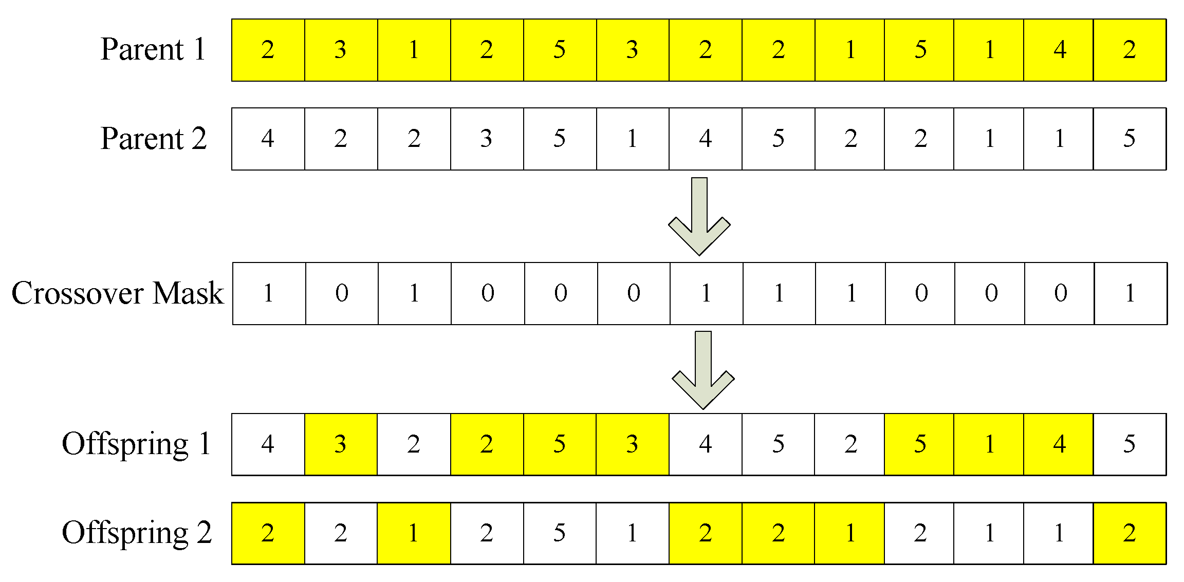
The uniform crossover was adopted in this research. As shown in Figure 2, the crossover operation includes two steps. The first step is to produce a crossover mask, and each gene in the chromosome corresponds to a crossover mask value. The crossover mask value is 0 or 1, and the value is randomly produced. The second step is to swap the values of genes for two parents when the corresponding crossover mask value is 1. If the crossover mask value is 0, the values of genes for two parents are not exchanged.

(2)

This study adopted the mutation operation according to the idea of a neighborhood. The neighborhood of the gene is considered as the incremental or decremental change to the integer values. An individual of the population is mutated with a probability. In a mutation operation, some genes of an individual are first randomly selected, and then these gene values are changed to their neighborhood.

(3)

In this research, the roulette selection method was employed as a selection mechanism, and the individual with a better fitness function value was more likely to be chosen as a parent to produce the offspring in the next generation.

6. Case Study

6.1. Case Introduction and Test Solving Algorithm

The industrial case of radio was applied for the case study. A producer of electronic products in Ningbo city plans to develop a product family of radio. The radio has been developed into a modular structure, and six mainly function modules are identified. The six function modules are the product case module (M1), the storage module (M2), the voice module (M3), the key module (M4), the control module (M5), and the display module (M6). There are several candidate module instances for each module, and different candidate instances of the same module have similar functionality but different performance. The customers in the market are surveyed and then grouped into three segments by clustering analysis, and the market demand of the three segments is estimated by market experts, as shown in

Table 3. Utility surpluses (USD) of similar products and market segment sizes.

	Market Segment 1	Market Segment 2	Market Segment 3
Demand quantity (PCS)	210,000	300,000	70,000
Utility of similar product 1	62.01	59.12	64.10
Utility of similar product 2	57.06	61.05	59.00
Utility of similar product 3	55.13	58.22	60.03

. By using conjoint analysis, the utility of each module instance can be obtained. Given some possible combinations, the orthogonal array selector provided in SPSS software was used to generate the number of some orthogonal product profiles. With the profiles, a fractional factorial experiment was designed to obtain the customer preferences. In the market, there were three similar products, and the surplus utilities of similar products were obtained by analyzing the product utility and the price, as shown in Table 3.

Table 4. Related information about module instances.

Module	Instance	Utility in Segment 1	Utility in Segment 2	Utility in Segment 3	Variable Unit Cost (USD)	Variable Unit Emission (g)	Weight (g)	GHG Emission (g)
M1	M1, 1	16.8	15.4	15.2	0.8	[0.23, 0.31]	120	[36.1, 37.5]
	M1, 2	17	15.6	15.2	0.8	[0.45, 0.53]	118	[32.5, 34.8]
	M1, 3	17.2	16	16	1	[0.28, 0.32]	119	[33.2, 36.4]
	M1, 4	17.2	16.7	14.9	1	[0.27, 0.34]	122	[35.2, 38.3]
M2	M2, 1	27.2	27.6	26.9	0.7	[0.08, 0.12]	78	[190, 198]
	M2, 2	27.3	28.6	26.9	0.8	[0.29, 0.31]	81	[208, 215]
	M2, 3	27.3	27.5	27.5	0.8	[0.09, 0.12]	84	[219, 228]
	M2, 4	27.3	27.5	28.7	0.9	[0.19, 0.22]	80	[200, 210]
M3	M3, 1	13.3	15	13.9	0.7	[0.47, 0.52]	92	[260, 272]
	M3, 2	13.2	15.2	14.3	0.7	[0.48, 0.54]	90	[248, 264]
	M3, 3	13.3	14.8	15	0.8	[0.29, 0.32]	93	[278, 288]
M4	M4, 1	11.3	11.3	11.1	0.6	[0.27, 0.33]	89	[297, 308]
	M4, 2	11.3	11.5	11.1	0.6	[0.09, 0.12]	92	[347, 358]
	M4, 3	11.5	11.5	11.5	0.8	[0.08, 0.14]	95	[262, 372]
M5	M5, 1	22.9	22.4	18.8	0.7	[0.17, 0.22]	101	[420, 431]
	M5, 2	23	22.8	20.2	0.8	[0.24, 0.38]	103	[422, 448]
	M5, 3	23.1	22.5	20.7	0.8	[0.33, 0.48]	104	[458, 464]
M6	M6, 1	19.2	17.2	17.2	0.6	[0.05, 0.2]	83	[136, 148]
	M6, 2	19.3	17.2	17.2	06	[0.19, 0.33]	81	[118, 128]
	M6, 3	19.3	17.1	17.3	0.6	[0.24, 0.38]	84	[143, 157]

shows the information about module instances. The variable unit cost of the module instance was evaluated by cost experts based on the assembly process. The variable unit emission of the module instance was estimated by experienced engineers based on the energy consumption in the assembly process. Through early evaluation, the information of candidate suppliers is shown in

Table 5. Information of suppliers.

Supplier Number	Available Module Instances (Purchase Price USD)	Distance (km)
S1	M1,1(4.8), M1,2(5.0), M1,3(5.1), M1,4(5.3), M3,1(6.5),M3,2(6.6), M3,3(6.6)	681
S2	M2,1(11), M2,2(11.3), M2,3(11.5), M4,1(5.3), M4,2(5.3),M4,3(5.4), M6,1(9.6), M6,2(9.7), M6,3(9.7)	1009
S3	M1,1(4.9), M1,2(5.1), M1,3(5.3), M1,4(5.4), M3,1(6.4), M3,2(6.5), M3,3(6.4), M5,1(11.6), M5,2(11.7), M5,3(11.8)	896
S4	M2,1(11.2), M2,2(11.3), M2,3(11.4), M4,1(5.2), M4,2(5.3), M4,3(5.3), M6,1(9.8), M6,2(9.9), M6,3(9.9)	987
S5	M1,1(4.9), M1,2(5.2), M1,3(5.3), M3,1(6.5), M3,2(6.5), M3,3(6.4)	1100
S6	M2,1(11.2), M2,2(11.4), M2,3(11.5), M2,4(11.6), M5,1(11.4), M5,2(11.5), M5,3(11.7)	756
S7	M2,1(11.3), M2,3(11.5), M2,4(11.7), M3,1(6.5), M3,2(6.6), M3,3(6.5)	653
S8	M1,1(4.8), M1,2(5.1), M1,3(5.3), M1,4(5.3), M3,1(6.5), M3,2(6.5), M3,3(6.5), M5,1(10.9), M5,2(11.2), M5,3(11.5), M6,1(9.9), M6,2(9.9), M6,3(9.9)	782
S9	M4,1(5.4), M4,2(5.5), M4,3(5.6), M5,1(11.7), M5,2(11.7), M5,3(11.8)	914
S10	M1,1(5), M1,3(5.2), M1,4(5.3), M3,1(6.4), M3,2(6.5), M3,3(6.4), M6,1(10), M6,2(10.1), M6,3(10.1)	1045
S11	M2,1(11.2), M2,3(11.4), M2,4(11.5), M4,1(5.5), M4,2(5.5), M4,3(5.5), M5,1(11.5), M5,2(11.6), M5,3(11.6)	995
S12	M3,1(6.3), M3,2(6.4), M3,3(6.5), M4,1(5.3), M4,2(5.4), M4,3(5.3), M5,1(11.5), M5,3(11.6)	745
S13	M2,1(10.9), M2,2(11.2), M2,3(11.3), M2,4(11.4), M5,1(11.8), M5,2(11.8), M5,3(11.7), M6,1(9.9), M6,2(10), M6,3(10)	925

.

Table 6. Discount information about suppliers.

Supplier Number	Sales Volume (in Thousand USD)	Discount Rate (%)
S1	(0, 300], (300, 600], (600, 900], (900, +∞)	0, 3, 5, 9
S2	(0, 200], (200, 400], (400, 600], (600, +∞)	0, 2, 7, 12
S3	(0, 500], (500, 600], (600, 900], (900, +∞)	0, 5, 8, 13
S4	(0, 150], (150, 400], (400, 1000], (1000, +∞)	0, 1, 5, 15
S5	(0, 300], (300, 600], (600, 800], (800, +∞)	0, 3, 8, 10
S6	(0, 200], (200, 500], (500, 800], (800, +∞)	0, 2, 5, 10
S7	(0, 600], (600, 600], (600, 1100], (1100, +∞)	0, 5, 10, 17
S8	(0, 250], (250, 500], (500, 800], (800, +∞)	0, 3, 5, 8
S9	(0, 200], (200, 900], (900, 1200], (1200, +∞)	0, 1, 7, 13
S10	(0, 500], (500, 800], (800, 1000], (1000, +∞)	0, 4, 7, 10
S11	(0, 300], (300, 600], (600, 900], (900, +∞)	0, 5, 10, 19
S12	(0, 300], (300, 600], (600, 1000], (1000, +∞)	0, 3, 5, 10
S13	(0, 150], (150, 750], (750, 900], (900, +∞)	0, 1, 5, 9

shows the discount information of the module instance given by candidate suppliers. By analyzing market and cost, the product price was estimated at (USD 49.7, USD 78.8). In the case study, the product price was discretized as a set of integer prices from USD 50 to USD 80. Based on the market price, C_Tr was 0.35 USD/km per ton. $[E_{Tr}^L,E_{Tr}^R]=[0.25,0.66]$, $E_z=\$\mathrm{15,000}$, and $F_z\in [485,510]$ were estimated by experienced engineers based on the energy consumption.

To solve the proposed optimization model, two metaheuristic algorithms including the genetic algorithm (GA) and the particle swarm optimization algorithm (PSO) were developed, and they were programmed in Matlab 2014b. For comparison purposes, two algorithms were used to calculate three test cases. The optimization conditions of three test cases were as follows:

Test cases 1–3: develop two product variants; d₁ = 0.75, d₂ = 0.25.

(1) Test case 1: u₁ = 0.48, u₂ = 0.52; (2) test case 2: u₁ = 0.5, u₂ = 0.5; (3) test case 3: u₁ = 0.52, u₂ = 0.48.

In the GA, the population size was set to 1000. The crossover rate was 0.8, and the mutation rate was 0.2. In the PSO algorithm, the inertia weight was set to 0.7. The cognition learning coefficient c₁ and the social learning coefficient c₂ were 1.49. The calculation results are shown in Figure 3. It can be observed that the GA outperformed the PSO algorithm for the proposed model. For example, in test case 1, the optimization results obtained using the GA were better than the optimization results obtained using the PSO in terms of profit and GHG emissions. Thus, the GA was used for solving the proposed optimization model. In test case 2, the weight combination of the two objective functions means that reducing GHG emissions was as important as profit. The fitness change curve of using the GA calculation is shown in Figure 4. The fitness value improved from generation to generation and became steady after approximately the 13th generation. The product configuration and order allocation of suppliers are given in

Table 7. Optimal results of test case.

Product Variant Configuration
Product variant 1	M1,4	M2,2	M3,1	M4,2	M5,2	M6,1
Product variant 2	M1,1	M2,4	M3,1	M4,1	M5,2	M6,3
Order Allocation Proportion
M1,1	S1:S3:S8 = 2:2:4
M1,4	S1:S3:S5:S8 = 3:2:5
M2,2	S2:S4:S6:S13 = 3:2:2:3
M2,4	S6:S7:S13 = 2:2:4
M3,1	S1:S3:S7:S8 = 4:3:2
M4,1	S2:S4:S11 = 1:4:2
M4,2	S2:S4:S9:S11 = 5:2:2
M5,2	S3:S6:S8:S9:S11:S13 = 3:2:1:3
M6,1	S4:S8:S13 = 1:3:4
M6,2	S2:S4:S8:S13 = 2:2:4
Profit: $1,068,426; GHG emission: 236,141.36 g

.

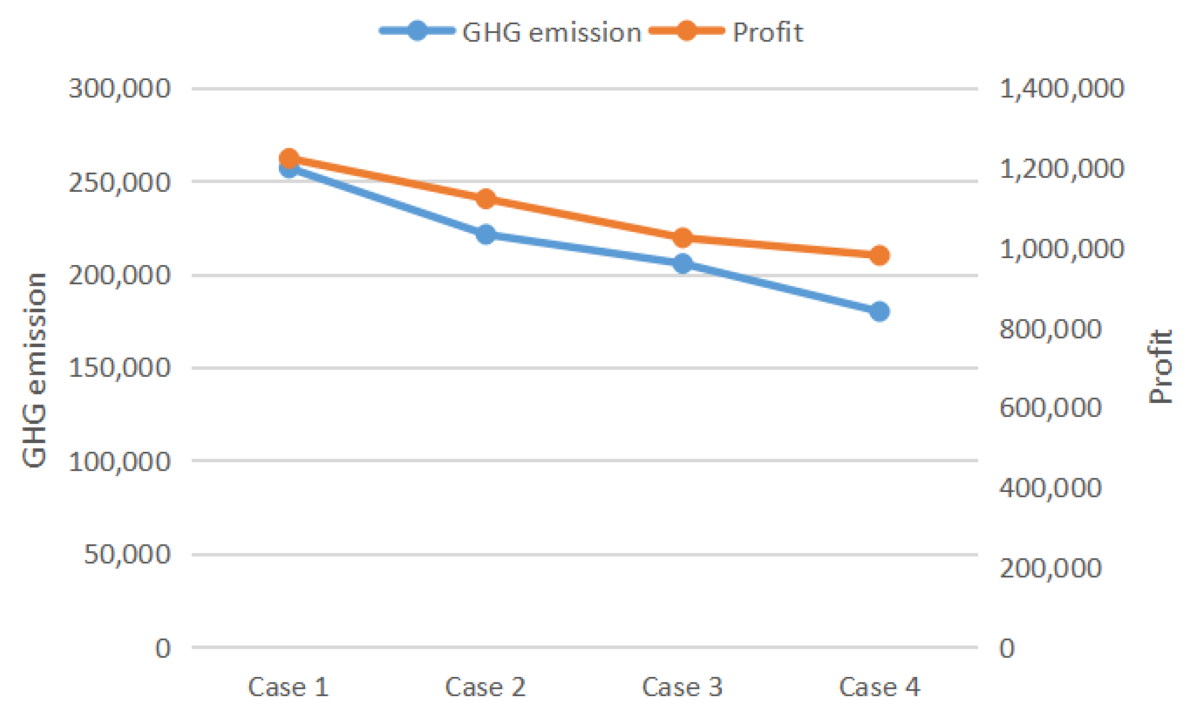
6.2. Sensitivity Analysis of GHG Emission Weight

Generally speaking, in product family design, the company not only wants to maximize profits but also wants to minimize GHG emissions. Nevertheless, the two goals are in conflict with each other. Therefore, enterprises must assign the weight for two objective functions. When more weight is assigned for the profit, the optimization solution can bring higher profit, but GHG emissions may be greater. Instead, when a greater weight is assigned to the GHG emissions, the optimization solution may lead to lesser GHG emissions and lesser profit. The following four different cases are discussed:

Cases 1–4: develop two product variants, d₁ = 0.85, d₂ = 0.15.

(1) Case 1: u₁ = 1, u₂ = 0; (2) case 2: u₁ = 0.8, u₂ = 0.2; (3) case 3: u₁ = 0.7, u₂ = 0.3; (4) case 4: u₁ = 0.5, u₂ = 0.5.

Figure 5 shows the optimal configurations of the two product variants for cases 1–4. It can be found that product family configuration in the four different cases are different. Except for different product configurations, the procurement plan of components in the four different cases was also different. The optimization results in cases 1–4 are given in Figure 6. It can be seen that there is a contradiction between GHG emissions and profit. When the profit is close to the optimal value, the GHG emissions value reaches the maximum. As the u₂ changes from 0 to 0.5, the GHG emissions value decreases by 35%, and the profit decreases by 18%. Through this experiment, it can be seen that it is necessary to set the weight of GHG emissions reasonably for reducing the environmental impacts of products.

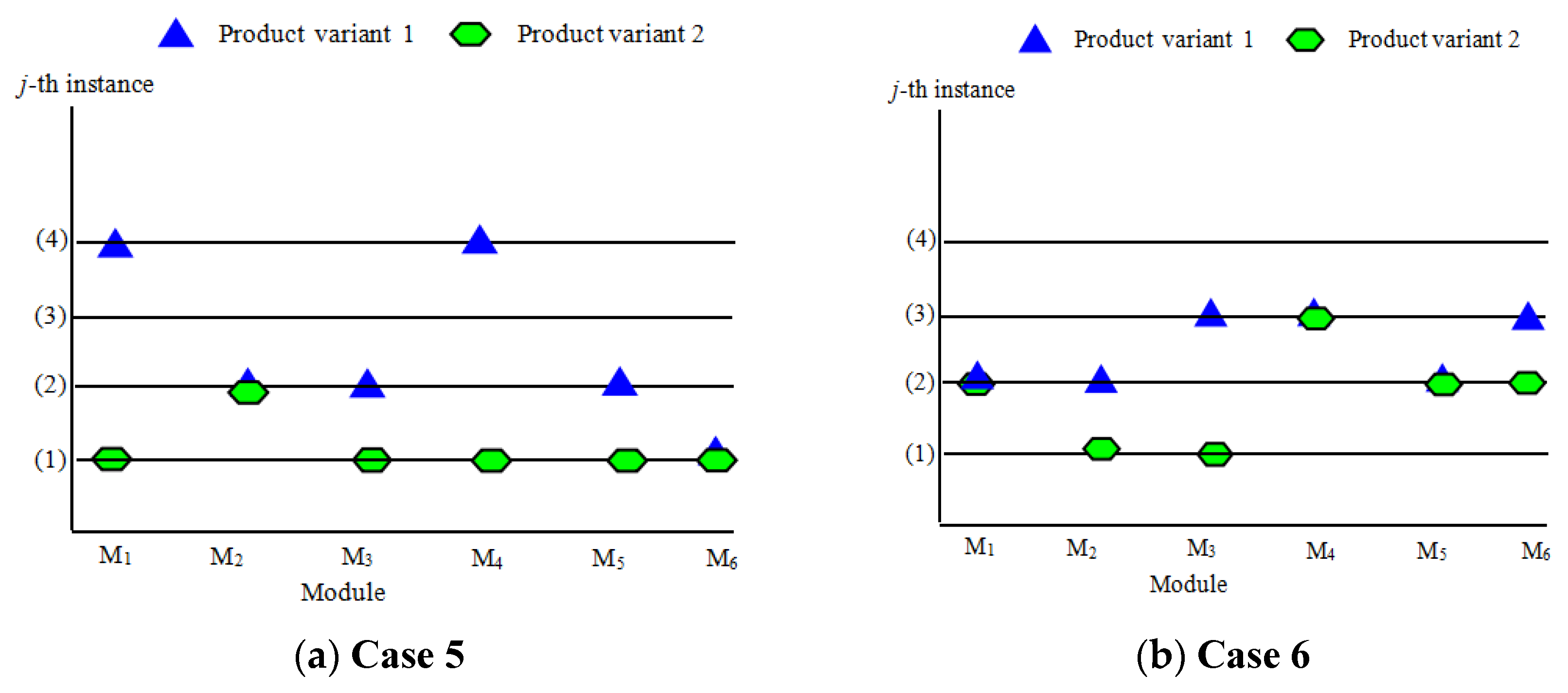
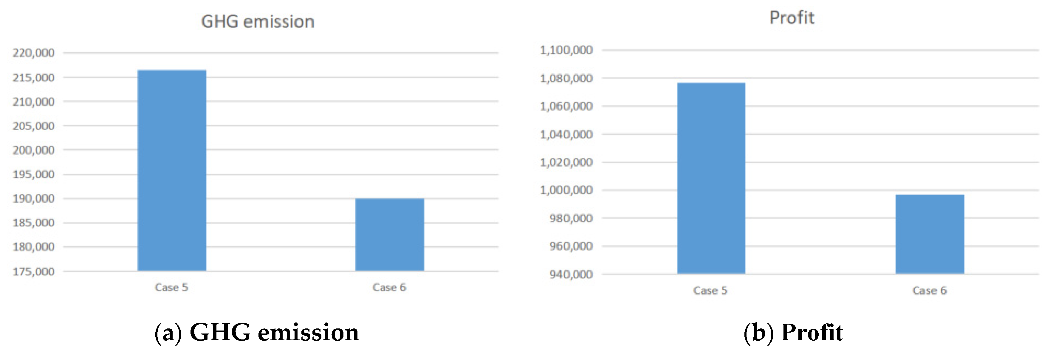
6.3. Sensitivity Analysis of Uncertain Weight (d₁, d₂)

The purpose of this section is to observe the influence of uncertain weight on optimization results, and two different cases are discussed:

• Case 5, case 6: develop two product variants; objective weight: u₁ = 0.7, u₂ = 0.3.
• Case 5: d₁ = 0.6, d₂ = 0.4;
• Case 6: d₁ = 0.4, d₂ = 0.6;

In this research, d₁ is the weight of the midpoint value (m(E^T)) for the uncertain optimization objective f₁, and d₂ is the weight of the radius (w(E^T)) of the uncertain optimization objective f₂. For comparative purposes, except for uncertain weight (d₁, d₂), other optimization conditions were the same in case 5 and case 6. The optimal product family configuration is shown in Figure 7. It can be seen that product configuration is different. For instance, in case 5, the module instances M_1,1, M_5,1, and M_6,1 were selected to configure the product family, and these module instances were not chosen in case 6. The relevant results of case 5 and case 6 are shown in Figure 8. With respect to GHG, the GHG emissions of the product family in case 5 were greater than that in case 6. The reason is that the weight d₁ in case 5 was greater than that in case 6. In fact, the midpoint value (m(E^T)) was similar to the average value of the uncertainty optimization objective function, and the radius value (w(E^T) of the objective function was similar to the deviation of the uncertainty optimization objective function. By optimizing the radius of the objective function, the objective function’s sensitivity to uncertain factors can be reduced, and it is to ensure the robustness of the design. Therefore, if designers pay more attention to the robustness of the design solution, they can assign a large weight to d₂. Similarly, with respect to profit, the profit in case 5 was greater than that in case 6. This is because the GHG emissions in case 5 were greater than those in case 6, and the two goals conflict with each other.

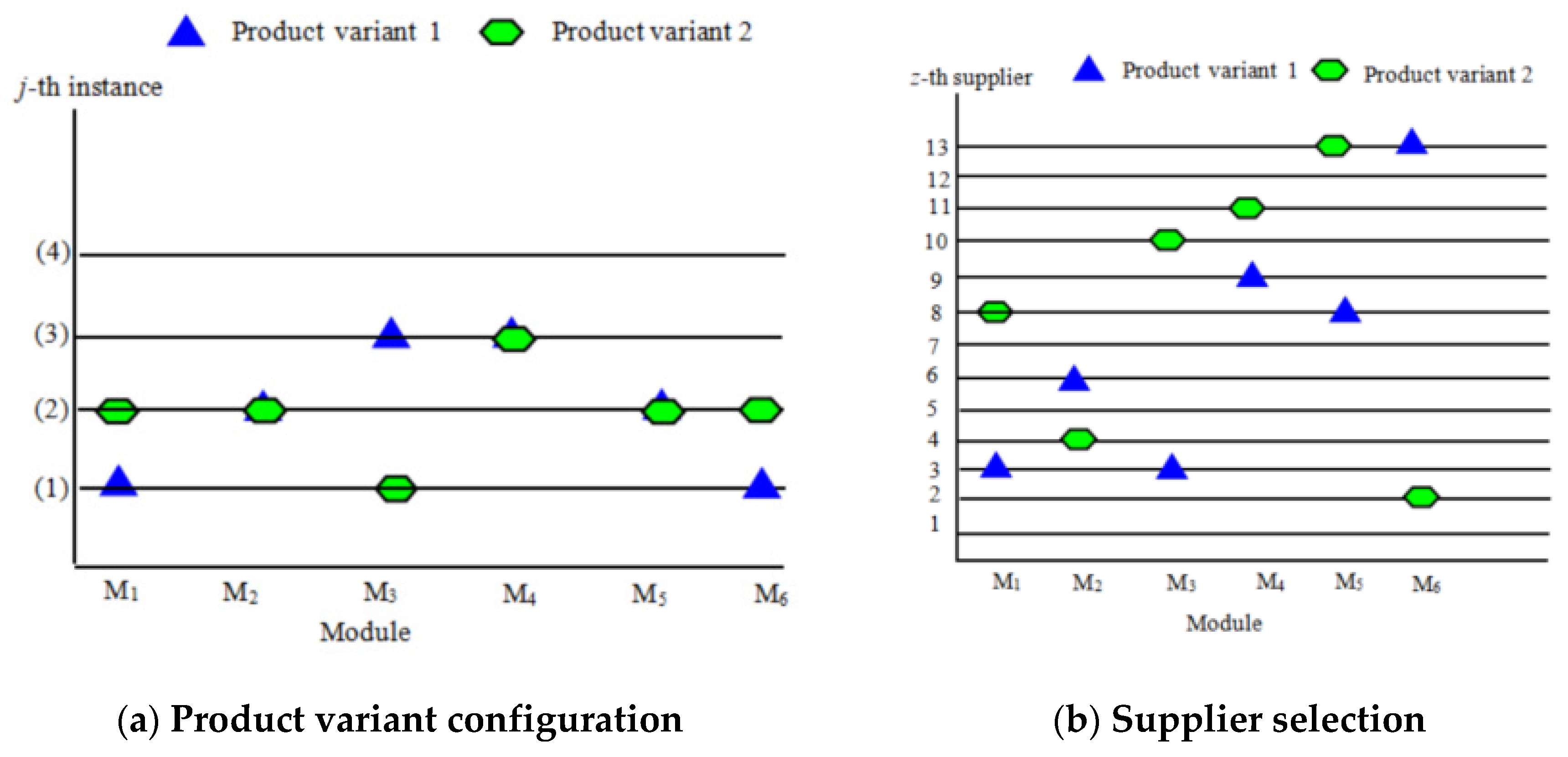
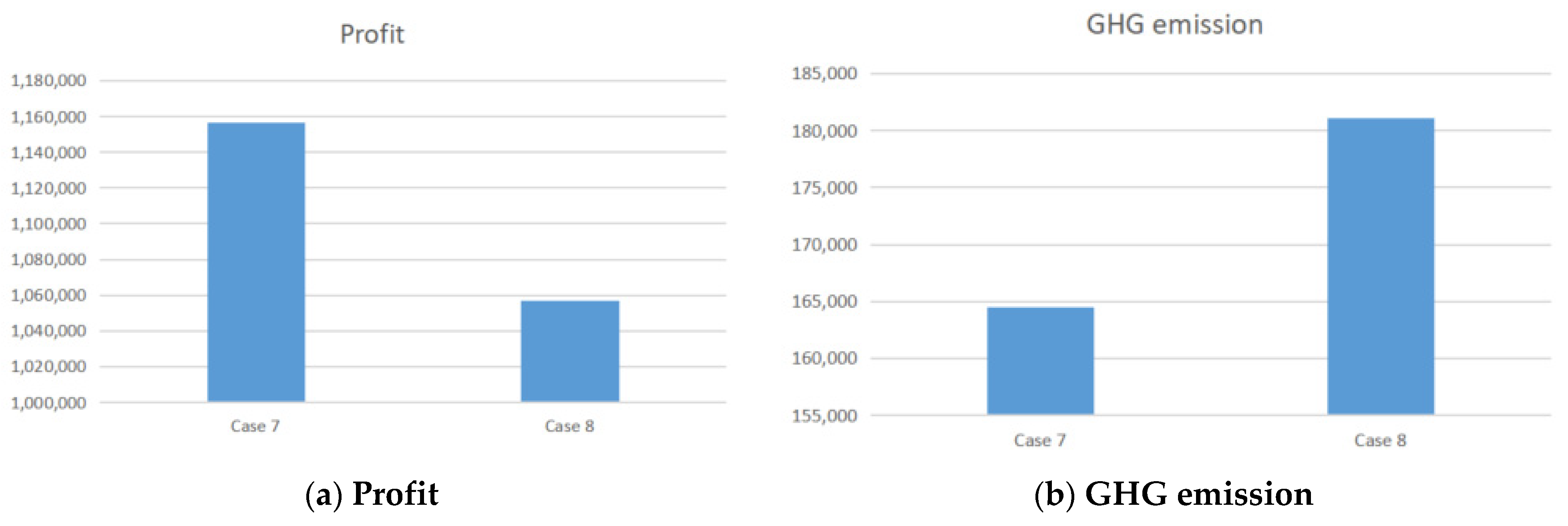
6.4. Compare Supplier Selection and Order Allocation in Product Family Design

No research has been reported in the literature dealing with the joint decision problem of product family design and order allocation of suppliers considering profit and GHG emissions. So it was not possible to compare our results with previous studies quantitatively. If some conditions or assumptions are ignored or changed in the proposed model, then this model and some previously models have the same base model. For example, if the order allocation of suppliers and uncertain GHG emissions were not considered, then the base of the proposed model reduces to Wang et al. [4]. If the issue of GHG emissions are ignored, and regardless of order allocation, then the base of the proposed model reduces to Cao et al. [27] and Luo et al. [26]. If the single product design is considered instead of product family design, and regardless of uncertain GHG emissions, then the proposed model has the same base model as Kuo et al. [9].

The purpose of this experiment was to compare the two optimization methods, and two different cases were discussed:

• Case 7, case 8: develop two product variants; objective weight: u₁ = 0.7, u₂ = 0.3; uncertain weight: d₁ = 0.65, d₂ = 0.35;
• Case 7: concurrent optimization of low-carbon product family design and supplier selection;
• Case 8: concurrent optimization of low-carbon product family design and order allocation.

The supplier selection was considered in the low-carbon product family design in case 7. In this case, regardless of the number of requirements, one module instance of one product variant was provided by a single supplier. In other words, only one supplier needs to be selected for each module of each product variant in the optimization process. Instead of just choosing a supplier, the total order allocation was considered in case 8, for example, assuming that M_1,1 is selected to configure two product variants (product variant 1 and product variant 2) in a product family. In case 7, it was possible that a supplier was selected to provide M_1,1 for configuring product variant 1, and another supplier was selected to provide M_1,1 for configuring product variant 2. Unlike case 7, the total demand of module instance M_1,1 was considered in case 8, and the total order was reasonably allocated to multiple suppliers who can provide module instance M_1,1 based on objective functions.

The optimal product family configuration and supplier selection is shown in Figure 9. Figure 10 shows the product family configuration and the optimal order allocation schemes in case 8. The product family configurations of case 7 and case 8 were different. The optimization results are shown in Figure 11. In case 7, not only the profit was higher than that in case 8 but also the GHG emission was less than that in case 8. This is because the order planning was not fully considered in case 7. If the order allocation is reasonable, more discounts from suppliers can be enjoyed by the firm. The experimental results showed that concurrent optimization of low-carbon product family design and order allocation could bring the company greater profit and lower GHG emissions than just considering supplier selection in product family design. Therefore, it is meaningful that the procurement plan of components is taken into account simultaneously in low-carbon product family design.

7. Conclusions

In recent years, many governments, non-profit organizations, and enterprises have formulated relevant standards to help enterprises in promoting carbon management and to encourage the design of low-carbon products. These standards include: ISO 14064, PAS 2050, and ISO/TS 14067. Many types of emission-regulation schemes have been suggested by UNCFC and the Kyoto Protocol to curb GHG emissions, such as carbon taxes and carbon cap-and-trade policies. Under these initiatives and the mounting pressure stemming from the implementation of the Kyoto Protocol and the Copenhagen protocol, enterprises have to take actions to reduce GHG emissions from their products. In addition to the pressure from government policy for environmental protection, another purpose for enterprises to design low-carbon products is to attract more consumers due to the fact that more and more consumers have begun to prefer low-carbon products. Low-carbon product design has become a hot topic in both academia and industry, and a multitude of researchers have focused on low-carbon product design.

The current research mainly focused on the low-carbon design method for a single product. At present, to meet the various needs of customers and to keep large-scale economic benefits, the production mode of enterprises has changed from mass production to mass customization. As a result, the product design method has changed from single product design to product family design. In recent years, some researchers have begun to study low-carbon product family design. Previous studies on low-carbon product family design have failed to consider the uncertainty of the related GHG emissions. In addition, the procurement planning of components was not fully considered. This study proposed a concurrence optimization model for low-carbon product family configuration and the procurement plan of components under uncertainty. In the model, the uncertain GHG emission data were considered as an interval number. In addition, the order allocation of a multi-supplier was also concerned in low-carbon product family design. To effectively solve the uncertain optimization model, the genetic algorithm was developed. A case study was implemented to demonstrate the effectiveness of the proposed approach. Our results provide several managerial insights: (1) companies/decision-makers can use the proposed model to simultaneously determine the product family design, the procurement strategy of components, and the price strategy of product variants based on the objectives of maximizing profit and minimizing GHG emissions under uncertainty. (2) There was a contradiction between GHG emissions and profit in low-carbon product family design and order allocation, so the decision-makers need to set the weight of each objective reasonably to reduce the environmental impacts of products. (3) In low-carbon product family design, the decision-makers can reduce GHG emissions of the product family by selecting appropriate suppliers and reasonably allocating orders, in addition to selecting low-carbon components. (4) The concurrent optimization of low-carbon product family design and order allocation can bring the company more profit and fewer GHG emissions than just considering supplier selection in low-carbon product family design. Hence, it is a great option to include the procurement plan of components in the product family design for an optimized low-carbon design scheme.

In view of the present limitations of our model, such as deterministic market demand, constant purchase price, and ignorance of the lead time and the supplier capacity, several extensions of this work are possible. The model can be extended to include stochastic market demands (see for reference Wang et al. [36]). In the model, we assumed that the purchase price is stable. However, if the international supply chain is considered, the purchase prices may fluctuate due to uncertain currency exchange rates (Gunay et al. [37]). In the model, the production cost was considered as a crisp value, and it can be extended to consider the fuzzy production cost (Kumar et al. [38]). The model can be further extended by adding a lead time constraint and a supplier capacity constraint (Ray et al. [39]; Hu et al. [40]). The study can also be extended by considering the variant production rate (Alkahtani et al. [41]), production quality improvement (see for reference Sarkar et al. [42]), inventory management with backorders, and preservation technology (Mishra et al. [43]; Yadav et al. [44]).

References

1. Intergovernmental Panel on Climate Change (IPCC). IPCC Fourth Assessment Report: Climate Change 2007; Cambridge University Press: New York, NY, USA, 2007; pp. 447–496. [Google Scholar]
2. Wang, Q.; Tang, D.B.; Yin, L.L.; Salido, M.A.; Giret, A.; Xu, Y.C. Bi-objective optimization for low-carbon product family design. Robot. Cim. Int. Manuf. 2016, 41, 53–65. [Google Scholar] [CrossRef] [Green Version]
3. Xiao, W.X.; Du, G.; Zhang, Y.Y.; Liu, X.J. Coordinated optimization of low-carbon product family and its manufacturing process design by a bilevel game-theoretic model. J. Clean. Prod. 2018, 184, 754–773. [Google Scholar] [CrossRef]
4. Wang, Q.; Tang, D.; Yin, L.; Ullah, I.; Salido, M.A.; Giret, A. An optimization method for coordinating supplier selection and low-carbon design of product family. Int. J. Precis. Eng. Manuf. 2018, 19, 1715–1726. [Google Scholar] [CrossRef]
5. Song, J.S.; Lee, K.M. Development of a low-carbon product design system based on embedded GHG emissions. Resour. Conserv. Recycl. 2010, 54, 547–556. [Google Scholar] [CrossRef]
6. Qi, Y.; Wu, X.B. Low-carbon technologies integrated innovation strategy based on modular design. Energy Procedia 2011, 5, 2509–2515. [Google Scholar] [CrossRef] [Green Version]
7. Su, J.C.P.; Chu, C.; Wang, Y. A decision support system to estimate the carbon emission and cost of product designs. Int. J. Precis. Eng. Manuf. 2012, 13, 1037–1045. [Google Scholar] [CrossRef]
8. Zhang, X.F.; Zhang, S.Y.; Hu, Z.Y.; Yu, G.; Pei, C.H.; Sa, R.N. Identification of connection units with high GHG emissions for low-carbon product structure design. J. Clean. Prod. 2012, 27, 118–125. [Google Scholar] [CrossRef]
9. Kuo, T.C.; Chen, H.M.; Liu, C.Y.; Tu, J.C.; Yeh, T.C. Applying multi-objective planning in low-carbon product design. Int. J. Precis. Eng. Manuf. 2014, 15, 241–249. [Google Scholar] [CrossRef]
10. Xu, Z.Z.; Wang, Y.S.; Teng, Z.R.; Zhong, C.Q.; Teng, H.F. Low-carbon product multi-objective optimization design for meeting requirements of enterprise, user and government. J. Clean. Prod. 2015, 103, 747–758. [Google Scholar] [CrossRef]
11. He, B.; Wang, J.; Huang, S.; Wang, Y. Low-carbon product design for product life cycle. J. Eng. Des. 2015, 26, 321–339. [Google Scholar] [CrossRef]
12. Chiang, T.A.; Che, Z.H. A decision-making methodology for low-carbon electronic product design. Decis. Support Syst. 2015, 71, 1–13. [Google Scholar] [CrossRef]
13. He, B.; Tang, W.; Wang, J.; Huang, S.; Deng, Z.Q.; Wang, Y. Low-carbon conceptual design based on product life cycle assessment. Int. J. Adv. Manuf. Technol. 2015, 81, 863–874. [Google Scholar] [CrossRef]
14. Zhang, C.; Huang, H.H.; Zhang, L.; Bao, H.; Liu, Z.F. Low-carbon design of structural components by integrating material and structural optimization. Int. J. Adv. Manuf. Technol. 2018, 95, 4547–4560. [Google Scholar] [CrossRef]
15. Tang, D.B.; Wang, Q.; Ullah, I. Optimisation of product configuration in consideration of customer satisfaction and low carbon. Int. J. Prod. Res. 2017, 55, 3349–3373. [Google Scholar] [CrossRef]
16. Kim, S.; Moon, S.K. Sustainable platform identification for product family design. J. Clean. Prod. 2017, 143, 567–581. [Google Scholar] [CrossRef]
17. Wang, Q.; Tang, D.; Li, S.; Yang, J.; Salido, M.A.; Giret, A.; Zhu, H. An optimization approach for the coordinated low-carbon design of product family and remanufactured products. Sustainability 2019, 11, 460. [Google Scholar] [CrossRef] [Green Version]
18. Jiao, J.; Tseng, M.M. A methodology of developing product family architecture for mass customization. J. Intell. Manuf. 1999, 10, 3–20. [Google Scholar] [CrossRef] [Green Version]
19. Du, X.; Jiao, J.; Tseng, M.M. Architecture of product family: Fundamentals and methodology. Concurr. Eng. 2001, 9, 309–325. [Google Scholar] [CrossRef]
20. Oivares-Benitez, E.; Gonzalez-Velarde, J.L. A meta-heuristic approach for selecting a common platform for modular products based on product performance and manufacturing cost. J. Intell. Manuf. 2008, 19, 599–610. [Google Scholar] [CrossRef]
21. Zacharias, N.A.; Yassine, A.A. Optimal platform investment for product family design. J. Intell. Manuf. 2008, 19, 131–148. [Google Scholar] [CrossRef]
22. Siddique, Z.; Rosen, D.W.; Wang, N. On the applicability of product variety design concepts to automotive platform commonality. In Proceedings of the ASME Design Engineering Technical Conferences, Atlanta, GA, USA, 13–16 September 1998. [Google Scholar]
23. Thevenot, H.J.; Simpson, T.W. Product Platform and Product Family Design: Methods and Applications; Springer: New York, NY, USA, 2005; pp. 107–129. [Google Scholar]
24. Huang, G.Q.; Zhang, X.Y.; Liang, L. Towards integrated optimal configuration of platform products, manufacturing processes, and supply chains. J. Oper. Manag. 2005, 23, 267–290. [Google Scholar] [CrossRef]
25. Huang, G.Q.; Zhang, X.Y.; Lo, V.H.Y. Integrated configuration of platform products and supply chains for mass customization: A game theoretic approach. IEEE Trans. Eng. Manag. 2007, 54, 156–171. [Google Scholar] [CrossRef] [Green Version]
26. Luo, X.G.; Kwong, C.K.; Tang, J.F.; Deng, S.F.; Gong, J. Integrating supplier selection in optimal product family design. Int. J. Prod. Res. 2011, 49, 4195–4222. [Google Scholar] [CrossRef]
27. Cao, Y.; Luo, X.G.; Kwong, C.K.; Tang, J.F.; Zhou, W. Joint optimization of product family design and supplier selection under multinomial logit consumer choice rule. Concurr. Eng. 2012, 20, 335–347. [Google Scholar] [CrossRef]
28. Khalaf, R.; Agard, B.; Penz, B. Simultaneous design of a product family and its related supply chain using a tabu search algorithm. Int. J. Prod. Res. 2011, 49, 5637–5656. [Google Scholar] [CrossRef]
29. Sr, A.; Ah, B.; Rzf, C. Concurrent design of product family and supply chain network considering quality and price. Transport. Res. E-LOG 2015, 81, 18–35. [Google Scholar]
30. Luo, X.G.; Li, W.; Kwong, C.K.; Cao, Y. Optimisation of product family design with consideration of supply risk and discount. Res. Eng. Des. 2016, 27, 37–54. [Google Scholar] [CrossRef]
31. Yang, D.; Jiao, J.X.; Ji, Y.J.; Du, G.; Helo, P.; Valente, A. Joint optimization for coordinated configuration of product families and supply chains by a leader-follower stackelberg game. Eur. J. Oper. Res. 2015, 246, 263–280. [Google Scholar] [CrossRef]
32. Hsu, T.H.; Chu, K.M.; Chan, H.C. The fuzzy clustering on market segment. In Proceedings of the IEEE International Conference on Fuzzy Systems, San Antonio, TX, USA, 7–10 May 2000. [Google Scholar]
33. Jiao, J.X.; Zhang, Y. Product portfolio planning with customer-engineering interaction. IIE Trans. 2005, 37, 801–814. [Google Scholar] [CrossRef] [Green Version]
34. Ishibuchi, H.; Tanaka, H. Multiobjective programming in optimization of the interval objective function. Eur. J. Oper. Res. 1990, 48, 219–225. [Google Scholar] [CrossRef]
35. Jiang, C.; Han, X.; Liu, G.R.; Liu, G.P. A nonlinear interval number programming method for uncertain optimization problems. Eur. J. Oper. Res. 2008, 188, 1–13. [Google Scholar] [CrossRef]
36. Wang, J.T.; Wang, L.W.; Ye, F.; Xu, X.J.; Yu, J.J. Order decision making based on different statement strategies under stochastic market demand. J. Syst. Sci. Eng. 2013, 22, 171–190. [Google Scholar] [CrossRef]
37. Gunay, E.E.; Park, K.; Kremer, G.O. Integration of product architecture and supply chain under currency exchange rate fluctuation. Res. Eng. Des. 2021, 32, 331–348. [Google Scholar] [CrossRef]
38. Kumar, S.; Sarkar, B.; Kumar, A. Fuzzy reverse logistics inventory model of smart items with two warehouses of a retailer considering carbon emissions. RAIRO—Oper. Res. 2021, 55, 2285–2307. [Google Scholar] [CrossRef]
39. Ray, S.; Jewkes, E.M. Customer lead time management when both demand and price are lead time sensitive. Eur. J. Oper. Res. 2004, 153, 769–781. [Google Scholar] [CrossRef]
40. Hu, X.L.; Motvvani, J.G. Minimizing downside risks for global sourcing under price-sensitive stochastic demand, exchange rate uncertainties, and supplier capacity constraints. Int. J. Prod. Econ. 2014, 147, 398–409. [Google Scholar] [CrossRef]
41. Alkahtani, M.; Omair, M.; Khalid, Q.S.; Hussain, G.; Sarkar, B. An agricultural products supply chain management to optimize resources and carbon emission considering variable production rate: Case of nonperishable corps. Processes 2020, 8, 1505. [Google Scholar] [CrossRef]
42. Sarkar, B.; Sarkar, M.; Ganguly, B.; Cardenas-Barron, L.E. Combined effects of carbon emission and production quality improvement for fixed lifetime products in a sustainable supply chain management. Int. J. Prod. Econ. 2021, 231, 107867. [Google Scholar] [CrossRef]
43. Mishra, U.; Wu, J.Z.; Sarkar, B. Optimum sustainable inventory management with backorder and deterioration under controllable carbon emissions. J. Clean. Prod. 2020, 279, 123699. [Google Scholar] [CrossRef]
44. Yadav, D.; Kumari, R.; Kumar, N.; Sarkar, B. Reduction of waste and carbon emission through the selection of items with cross-price elasticity of demand to form a sustainable supply chain with preservation technology. J. Clean. Prod. 2021, 297, 126298. [Google Scholar] [CrossRef]
Figure 1. An example of a chromosome.
Sustainability 13 10764 g001
Figure 2. An example of crossover.
Sustainability 13 10764 g002
Figure 3. The optimization results of the GA and the PSO.
Sustainability 13 10764 g003
Figure 4. Convergence curve of fitness value.
Sustainability 13 10764 g004
Figure 5. Optimized product family configuration for cases 1–4.
Sustainability 13 10764 g005
Figure 6. Optimized results for cases 1–4.
Sustainability 13 10764 g006
Figure 7. Optimized product family configuration for cases 5–6.
Sustainability 13 10764 g007
Figure 8. Optimized results for cases 5–6.
Sustainability 13 10764 g008
Figure 9. Optimized product family configuration and supplier selection for cases 7.
Sustainability 13 10764 g009
Figure 10. Optimized product family configuration and order allocation proportion of suppliers for case 8.
Sustainability 13 10764 g010
Figure 11. Optimized results for cases 7–8.
Sustainability 13 10764 g011