Optimal Load Frequency Control of Island Microgrids via a PID Controller in the Presence of Wind Turbine and PV

Abstract

This article studied the load frequency control (LFC) of a multi-source microgrid with the presence of renewable energy sources. To maintain a sustainable power supply, the frequency of the system must be kept constant. A Proportional–Integral–Derivative (PID) controller is presented as a secondary controller to control the frequency of the microgrid in island mode, and the integral of squared time multiplied by error squared (ISTES) is used as a performance index. The use of the Craziness-Based Particle Swarm Optimization (CRPSO), which is an improved version of Particle Swarm Optimization (PSO), improves the convergence speed in optimizing the nonlinear problem of load and frequency controller design. The test microgrid is composed of the load and distributed generation units such as diesel generators, photovoltaics and wind turbines. The proposed controller provided the desired response to adjusting the microgrid frequency, achieving the final response after a short time and making it more stable and less oscillatory compared with the conventional system.

1. Introduction

Nowadays, with the reduction of fossil fuel sources and increasing pollution and global warming, the use of renewable energy to generate electricity is one of the best solutions available [1,2,3]. Although these energies have many advantages, the stability of the power system, and especially the microgrids, is associated with problems for which proper control must be exercised [4,5]. One of the most widely used and economical renewable energy sources is wind energy, which is accessible through wind turbines. On the other hand, the issue of microgrid sustainability has become one of the main challenges of the electricity industry [6,7]. By upsetting the balance between production and demand, the microgrid frequency undergoes changes such that if the load decreases and the output is increased, the generator tends to increase its speed and frequency, and if the load increases and production decreases, the generator speed and frequency reduce. Therefore, the microgrid frequency can be used as an indicator to maintain the real power balance [8,9].

The use of renewable energy is increasing. Meanwhile, the use of wind energy has grown significantly around the world [10,11]. Most turbines used in wind farms are of the constant speed type, but the use of variable speed wind turbines is expanding significantly. The advantages of wind turbines equipped with variable speed turbines include the ability to track the maximum power point, separate control of reactive power, less mechanical stress and smaller size of the converters [12,13,14]. The doubly fed induction generator (DFIG) is commonly used in variable speed wind farms due to lower installation costs, higher efficiency and lower losses [15,16].

Effective performance and control are important aspects of the microgrid management challenge. Microgrid control is generally performed at three levels, including primary, secondary and tertiary, which are described in [17,18]. The first two control levels are related to voltage and frequency drop control and reset the system even in island mode when the load or output changes. The third control level determines and manages the microgrid components and determines their interaction with the main network in such a way that the economic aspects and reliability of the system are considered. Detailed discussions on the microgrid controller’s architecture with decentralized controllers are available in [19,20], while discussions can be found for centralized controllers in [21,22] and hybrid microgrids in [23,24]. There are also methods for solving microgrid scheduling and management that focus on the exact model of microgrid components and the effect of uncertainties on them, such as deterministic methods in [25,26] and possible methods in [27,28].

In [29], the authors conducted research for the control of island microgrids to reduce the frequency and power fluctuations and in [30] for intelligent frequency control for an AC microgrid or a combination of the particle swarm algorithm and fuzzy logic. In [31], the authors focused on the stability and control of the microgrid, which included a combination of microturbines, fuel cells and electrolyzers and was self-regulated by a fuzzy controller. In [32], the state feedback method for hybrid microgrid stability analysis by finding system eigenvalues and adjusting controller parameters was studied. In [33], a new control method for microgrid frequency control including solar panels and wind turbines was proposed. In [34], microgrid frequency control using the inertial sampling method with an additional control is presented. In [35], the load frequency control of a multi-zone power system in the presence of DFIG was studied, and in [36], a study of microgrids with back-to-back converters is presented. In [37], frequency control of island microgrids including energy storage sources by the differential evolution algorithm was proposed, in which the lack of controller design was conducted by considering the uncertainties. In [38], a study of Control of greenhouse gas emissions by optimal DER technology investment and energy management in zero-net-energy buildings.

Each microgrid can continue to operate in both island and grid-connected modes. In the case of network connection due to the high inertia of the power system, the stability of the network does not fluctuate much with the presence of small disturbances, while in island mode, due to the low inertia of the network, with small disturbances or even a load change, the microgrid frequency fluctuates. In this research, first, the microgrid frequency stability in island mode with a wind turbine with DFIG is investigated by applying small perturbations such as microgrid load changes. This microgrid has different types of distributed generation sources such as photovoltaics, fuel cells and diesel generators. In order to improve the microgrid frequency control, the PID frequency controller will be applied to the turbine model and the diesel generator governor model. Additionally, in order to improve the performance of the proposed controller, its gains are optimally adjusted using Craziness-Based Particle Swarm Optimization (CRPSO). The optimization objective function is determined to reduce frequency fluctuations in the short run. Therefore, the innovations of this article can be summarized as follows:

• Simultaneous optimization of PID control coefficients for an island microgrid with a wind turbine equipped with a two-way induction generator;
• The use of Craziness-Based Particle Swarm Optimization (CRPSO), which is an improved version of Particle Swarm Optimization (PSO) and is used to improve the convergence speed in optimizing the nonlinear problem of load and frequency controller design;
• Using the appropriate objective functions to reduce the settling time, maximum overshoot value and undershoot value.

2. Materials and Methods

Frequency modeling of island microgrids based on the block diagram connection of each of the distributed generation sources and a wind turbine equipped with DFIG is presented to investigate the frequency behavior of the system. Then, using the optimal adjustment of the PID controller with the CRPSO algorithm, the optimal frequency control method in the presence of DFIG is described step by step. In the optimization objective function, in order to reduce the parameters of the time domain in the form of the ISTSE objective function, the frequency error is selected so that the frequency fluctuations are damped after a while. The use of resources in microgrids will be realized to improve the frequency stability of microgrids. In addition, the application of the proposed controller in the microgrid and the optimal adjustment of its parameters will cause the microgrid frequency fluctuations to be well damped due to disturbances such as overload and will not prevent the microgrid from functioning.

2.1. Microgrid Load Frequency Control

The correct operation of the microgrid requires a balance of production power with the total power consumption and losses. Over time, the operating point of the system constantly changes, so the frequency and power allocated to the units may be skewed. These deviations can cause unwanted effects on the microgrid. Load frequency control (LFC), along with automatic production control, is one of the most important challenges in the design and operation of microgrids, which is necessary for the optimal performance of the microgrid and should be seriously considered in the design. The main objectives in controlling the LFC of the microgrid can be summarized as follows: ensure that the frequency deviation is zero in the island mode, reduce frequency fluctuations when changing the status from network connection mode to island mode and vice versa, proper tracking of loads and disturbances, minimize the amount of settling time and identify the maximum overshoot value and undershoot value when deviating in frequency.

2.2. Microbridge Frequency Response Modeling

The microgrid is inherently nonlinear and variable with time. The linearized model of the system can be used to investigate and analyze the frequency response of the microgrid to small load perturbations. The dynamics of the microgrid frequency response are much slower than the voltage and angle dynamics of the rotor and range from a few seconds to several minutes. Therefore, a simpler model is used to model the frequency behavior of the power system relative to perturbations, and they are much simpler than existing models for analyzing and simulating other types of dynamics. In most studies, to investigate the frequency behavior of microgrids, distributed generation sources are modeled with a first-order pre-phase transfer function. In the following, the microgrid frequency response model and some distributed generation sources are described.

2.3. Power and System Frequency Deviation

In order to maintain the stability of an independent system, the total output power must be effectively equal to the total power of the loads connected to the system. This strategy is in accordance with the following equation with the difference between the required power ($P_s^{*}$) and the total production power ($P_s$) [8,9]:

$$\Delta P_e=P_s^{*}-P_s$$

(1)

Since the frequency changes as the power changes, the frequency changes are determined by Equation (2):

$$\Delta f=\frac{\Delta P_e}{K_{sys}}$$

(2)

where $K_{sys}$ is the frequency characteristic constant of the system. Because there is a delay between frequency changes and power deviation, the transfer function for system frequency changes in terms of per unit frequency deviation can be determined by Equation (3) [29]:

$$G_{sys}=\frac{\Delta f}{\Delta P_e}=\frac{1}{K_{sys}\left(1+s{T}_{sys}\right)}=\frac{1}{D+sM}$$

(3)

where $D$ is the damping ratio and $M$ is the machine inertia of the microgrid.

2.4. Diesel Generator

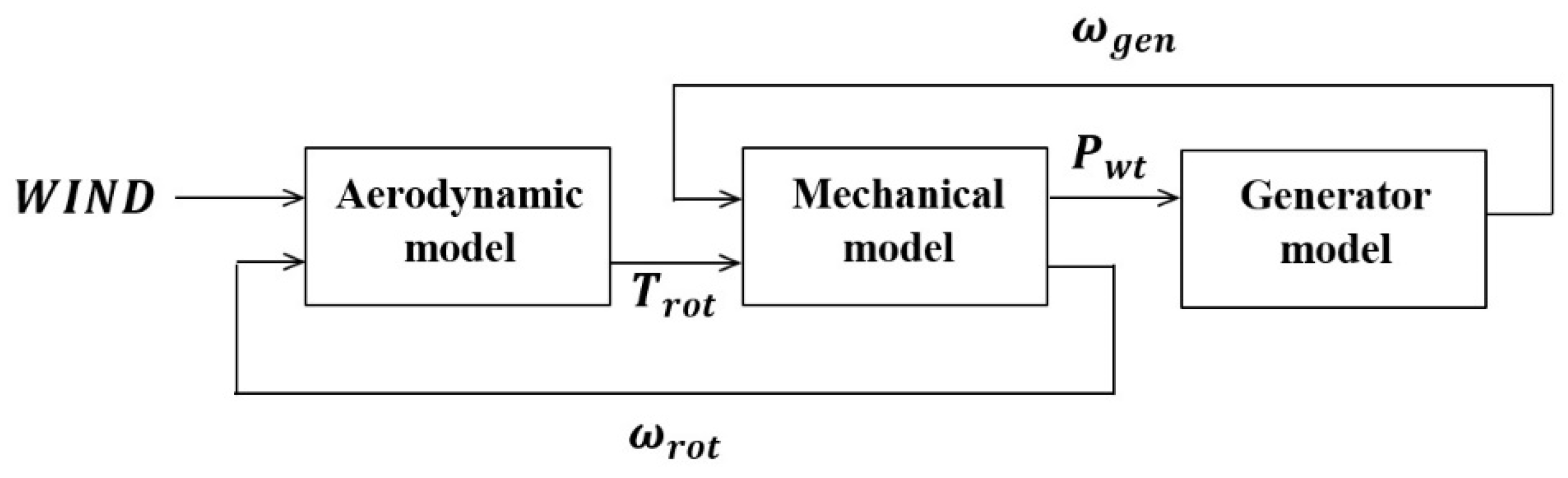
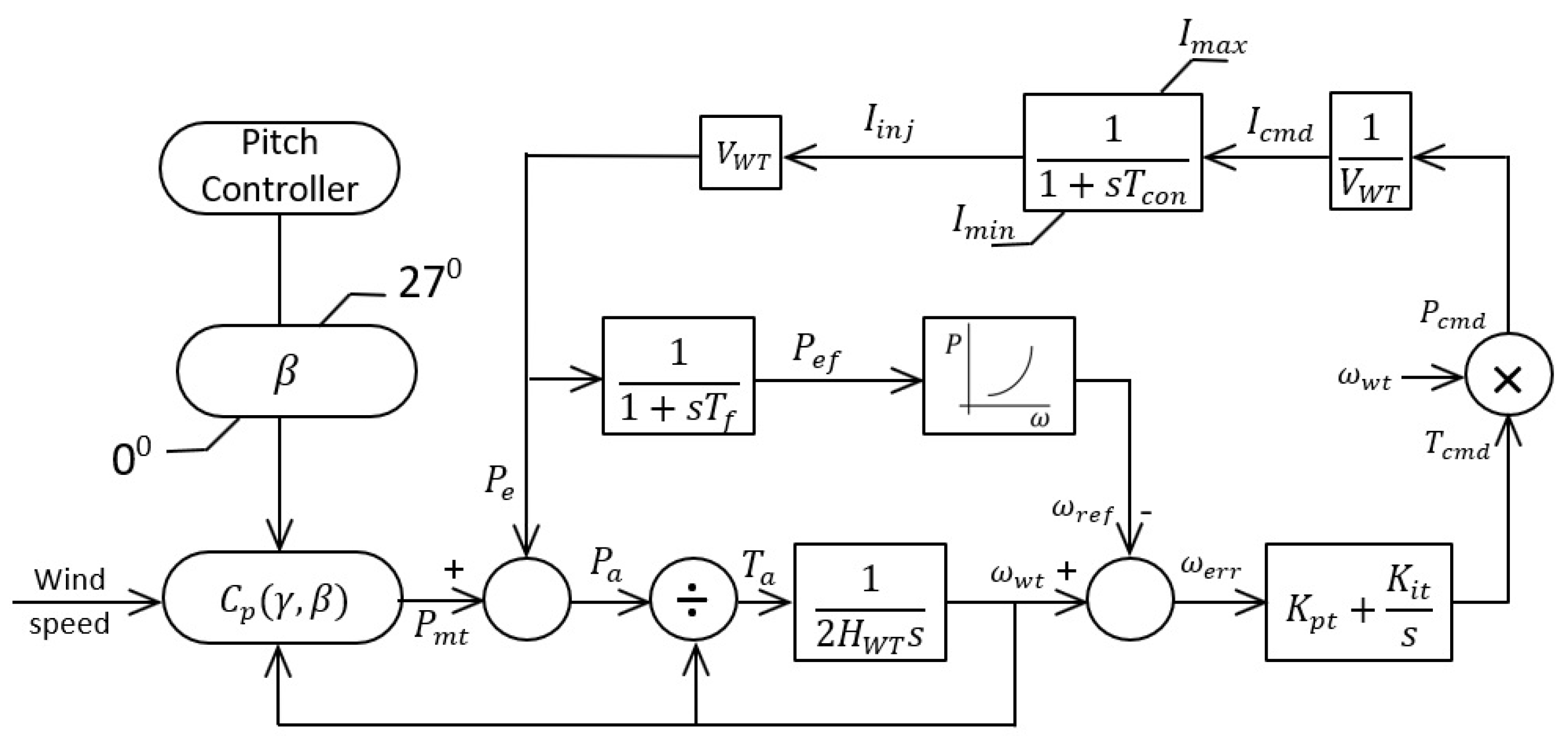
Diesel generators, like thermal turbogenerators, are equipped with a turbine and governor system. The first-order model of the generator, turbine and governor are given by Equations (4)–(6):

$$G_{DEG}(s)=\frac{K_{DEG}}{1+s{T}_{DEG}}=\frac{\Delta P_{DEG}}{\Delta f}$$

(4)

$$G_g(s)=\frac{1}{1+sT{g}_i}$$

(5)

$$G_{Turb}(s)=\frac{1}{sT}$$

(6)

where $K_{DEG}$ and $T_{DEG}$ are the gain and time constant of the transfer function of the diesel generator, respectively, and $T{g}_i$ and $T$ are the time constant of the governor and turbine of the diesel generator, respectively.

2.5. Wind Turbine

The first-order transfer function for the frequency model of wind power generation is given by Equation (7) [13]:

$$G_{WTG}(s)=\frac{K_{WTG}}{1+s{T}_{WTG}}=\frac{\Delta P_{WTG}}{\Delta P_w}$$

(7)

where $K_{WTG}$ and $T_{WTG}$ are the gain and the time constant of the transfer function of the equivalent wind turbine generator, respectively. The mechanical power relations of the wind turbine (Pw) in the fixed-speed wind turbine model are described in detail in the next section. Figure 1 shows the fixed-speed wind turbine model, which consists of three parts: the aerodynamic model, mechanical model and asynchronous generator model.

The aerodynamic torque due to wind force on the turbine blades is determined by Equation (8):

$$T_{rot}=\frac{1}{{\omega }_{rot}}{C}_P\left(\frac{\rho \pi R^2{v}^3}{2}\right)$$

(8)

where $C_P$ is the wind turbine power coefficient specified by Equation (9). The power coefficient shows how efficiently a turbine converts the energy in the wind to electricity [13]:

$$C_P=\left(0.44-0.0167\beta \right)\sin \left[\frac{\pi \left(\lambda -3\right)}{15-0.3\beta }\right]-0.0184\left(\lambda -3\right)\beta$$

(9)

where $\beta$ is the pitch angle of the turbine in terms of radians. The tip speed ratio of the turbine ($\lambda$) is determined by Equation (10):

$$\lambda =\frac{R{\omega }_{rot}}{v}$$

(10)

where $R{\omega }_{rot}$ is the blade tip speed in m/s and $v$ is the wind speed in m/s.

The mechanical model of a wind turbine, which includes the connection of the turbine shaft and the generator shaft, is usually considered as two- and three-part components, and their equations are taken into account. However, in some cases, due to the slow dynamics of the mechanical part versus the fast dynamics of the electrical part or the unavailability of all the necessary parameters to simulate the mechanical model, the dynamics of the mechanical part are generally ignored. Therefore, in most studies, the gearbox model is ignored, the shaft is considered as a rigid body, and the mechanical model is simplified with the following differential equation:

$$\frac{d{\omega }_A}{dt}=\frac{{\omega }_0}{2H_A}\left[T_{Am}-T_{Ae}-\frac{D_A}{{\omega }_0}{\omega }_A\right]$$

(11)

where ${\omega }_0$ and ${\omega }_A$ are the synchronous speed and the electric speed of the generator, respectively. In addition, $T_{Am}$ and $T_{Ae}$ are the mechanical and electrical torque. $H_A$ is the inertia, and $D_A$ is the damping coefficient of an asynchronous generator. A constant speed can contribute to network inertia response, like synchronous machines, but this is not the case with variable-speed wind turbine generators. An additional control loop is therefore needed to increase the actual output power during frequency perturbation (Figure 2).

2.6. Solar PV

The output power and linear form (frequency model) of the solar cell (photovoltaic) are determined by Equations (12) and (13):

$$P_{PV}=\eta S\Phi \left\{1-0.005\left(T_a+25\right)\right\}$$

(12)

$$G_{PV}(s)=\frac{K_{PV}}{1+s{T}_{PV}}=\frac{\Delta P_{PV}}{\Delta \Phi }$$

(13)

where $\Phi$ is the solar radiation in kw/m², $\eta$ is the conversion efficiency of the solar cell (9–12%) and $s$ is the surface area of the solar cell in square meters. In addition, $K_{PV}$ and $T_{PV}$ are the gain and time constant of the photovoltaic transfer function, respectively.

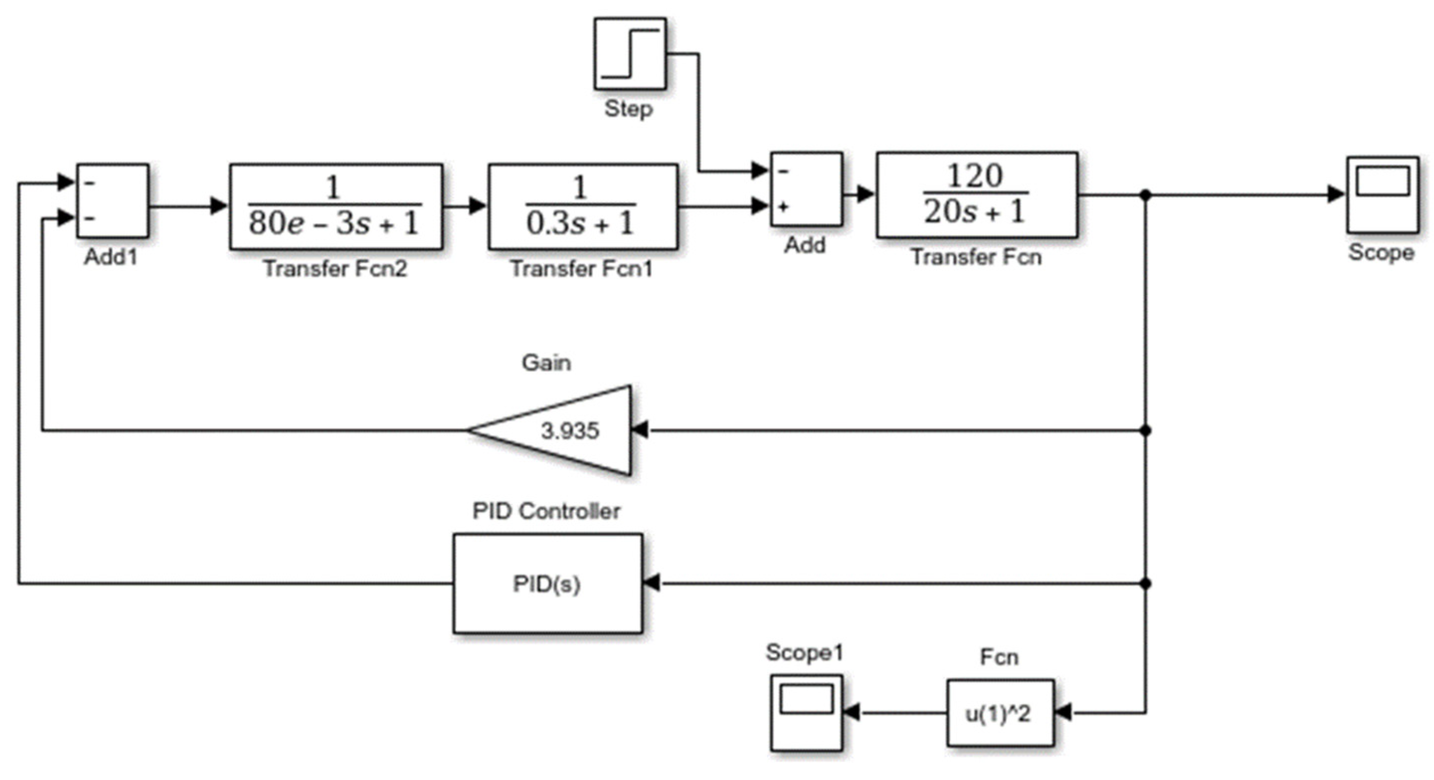
2.7. Load Frequency Control (LFC)

In the study of LFC, a step input is used to model the load changes. To analyze the response of the LFC system to a step load change, we first considered the state in which the speed changer was in a certain position. The output of the control system $\Delta F\left(s\right)$.

where $\Delta P_c=0$ is as follows:

$$\Delta F\left(s\right)=\frac{K_p}{1+S{T}_p}\left[\frac{-1}{R}\Delta F\left(s\right)\frac{1}{\left(1+S{T}_g\right)\left(1+S{T}_t\right)}-\frac{\Delta P_L}{S}\right]$$

(14)

According to the final value theorem, the steady state response of the system is

$$\Delta F=\lim \left[S\Delta F\left(s\right)\right]=\frac{R{K}_p}{R+K_p}\Delta P_L=-\frac{\Delta P_L}{\beta }$$

(15)

This relationship shows the frequency changes due to load changes.

In order to keep the system frequency constant, the steady state frequency deviation $\Delta F$ must be reduced to zero in exchange for load changes, and as can be seen, a speed changer must be used to achieve this goal. To bring the frequency to the nominal value, it is necessary to use an integrator as a second feedback loop, because the integral unit considers the mean error for a period of time and can eliminate it completely.

It can be seen that the frequency error signal is generated after amplification by the integral gain $K_L$ through the integrator with $\Delta P_c$ :

$$\begin{array}{l}\Delta P_{ref}=-K_L{\int }^{ }\Delta fdt\\ \Delta F\left(s\right)=-\frac{K_p}{T_p}\frac{\Delta P_L}{S^2+\left(\frac{K_p/R+1}{T_p}\right)s+\frac{K_1{K}_p}{T_p}}\end{array}$$

(16)

Applying the final value theorem yields

$$\begin{array}{l}\Delta F=s\Delta F\left(s\right)=0\\ S\to 0\end{array}$$

(17)

Therefore, the second feedback loop increases the frequency exponential error by increasing the degree of the system. However, the response dynamics of the system depend on the roots of the quadratic equation of the denominator of the following relation:

$$\Delta F\left(s\right)=-\frac{K_p}{T_p}\frac{\Delta P_L}{S^2+\left(\frac{K_p/R+1}{T_p}\right)s+\frac{K_1{K}_p}{T_p}}$$

(18)

By examining this equation, it is found that the response speed improves with increasing the value of $K_I$, but the fluctuations increase in the case of an excessive increase, and the system may become unstable. On the other hand, decreasing it leads to slowing down the response. Therefore, the integral gain must be adjusted to create a suitable position for the response.

2.8. Objective Function and Optimization with CRPSO

The speed update equation, taken from [30], can be obtained with the following equation:

$$\begin{array}{l}{\nu }_i{}^{k+1}=r_2\times {\nu }_i{}^k+\left(1-r_2\right)\times c_1\times r_1\times \left(P_{Best,I}-x_i{}^k\right)\\ +\left(1-r_2\right)\times c_2\times \left(1-r_1\right)\times \left(g_{Bes}-x_i{}^k\right)\end{array}$$

(19)

Global and local searches are balanced by a random number $\left(r_2\right)$ as described in the previous reference. Speed reversal can be modeled as follows:

$$\begin{array}{l}{\nu }_i{}^{k+1}=r_2\times sign\left(r_3\right)\times {\nu }_i{}^k+\left(1-r_2\right)\times c_1\times r_1\times \left(P_{Best,I}-x_i{}^k\right)\\ +\left(1-r_2\right)\times c_2\times \left(1-r_1\right)\times \left(g_{Bes}-x_i{}^k\right)\end{array}$$

(20)

In Equation (23), $sign\left(r_3\right)$ can be defined as follows:

$$sign\left(r_3\right)=\{\begin{array}{c}-1 r_3\le 0.05\\ 1 r_3>0.05\end{array}$$

(21)

For incorporating craziness, variation in the path of invading birds or fish movement can be controlled in conventional PSO with a craziness probability. Particles can go crazy according to the following equation before updating the position:

$${\nu }_i{}^{k+1}={\nu }_i{}^{k+1}+Pr\left(r_4\right)\times sign\left(r_4\right)\times {\nu }_i{}^{craziness}$$

(22)

where $Pr\left(r_4\right)$ and sign($r_4$) are defined as follows:

$$Pr\left(r_4\right)=\{\begin{array}{c}1 r_4\le P_{craz}\\ 0 r_4>P_{craz}\end{array}$$

(23)

$$sign\left(r_4\right)=\{\begin{array}{c}1 r_4\le 0.5\\ -1 r_4<P_{craz}\end{array}$$

(24)

The position update equation can be expressed as

$$x_i{}^{k+1}=x_i{}^k+{\nu }_i{}^{k+1}$$

(25)

The objective function in frequency control problems of power systems is generally performed as the sum of frequency deviations in areas of the system with appropriate balancing coefficients. In some articles, some parameters of the frequency and time response, including the settling time, maximum overshoot value, undershoot value and peak time are considered. This paper uses the integral of squared time multiplied by error squared (ISTES) objective function to simultaneously mitigate the frequency deviations and minimize the time response characteristics of the frequency. Therefore, in order to achieve the control goal (reduction of microgrid frequency fluctuations), microgrid frequency deviation must be minimized. In this research, the following objective function was used:

$$f={\int }_0^{t_{sim}}{\tau }^2\Delta f^{2}d\tau$$

(26)

Optimization of the PID controller parameters was performed with the CRPSO algorithm and with the above objective function. Optimization was performed with 100 particles and 100 repetitions to achieve the appropriate response. The steps for setting the PID coefficients are summarized as follows:

• Model the microgrid frequency response;
• Initialization of particles (PID coefficients are selected between 0 and 5);
• Execute the Simulink file of the frequency model and send the frequency response of the microgrid to calculate the objective function;
• Calculate the objective function for the PID coefficients of each particle;
• Determine the best local and global particle;
• Update the particle speed;
• Update the positions of the particles;
• Calculate the objective function for the PID coefficients of each particle;
• If the condition of stopping the algorithm (maximum repetition) is not met, repeat the steps from step 5;
• If the condition of stopping the algorithm is met, end the optimization operation and select the best global particle as the optimized PID coefficients.

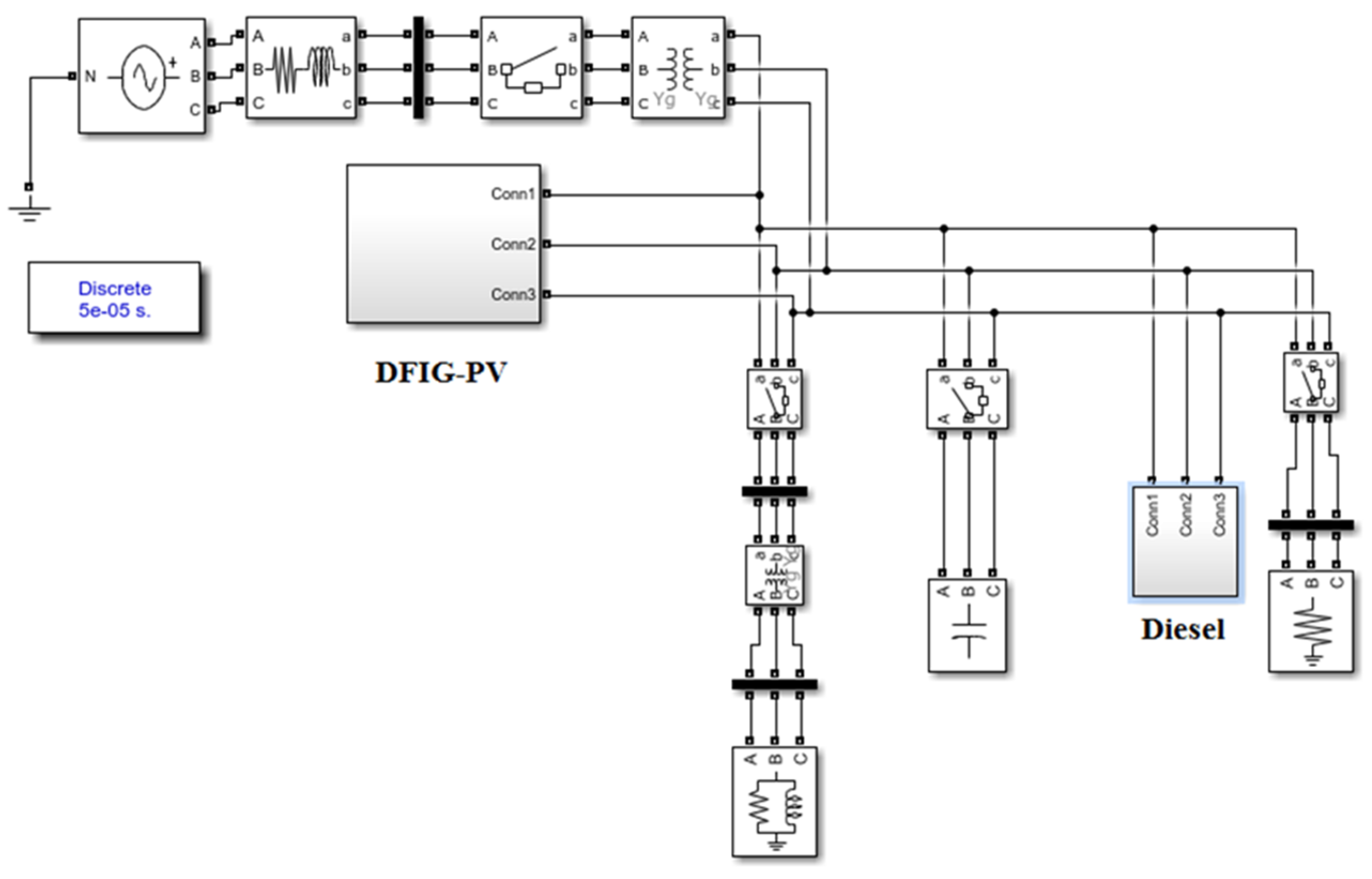
2.9. Studied System

The microgrid can be operated in two modes: islanded and grid-connected. The overall structure of the microgrid is shown in Figure 3, which includes the DFIG wind turbine, solar system, diesel generator and load. The microgrid and the national network would be connected at the common connection point. The sources used in these networks are connected to each other by electronic elements. In fact, in these microgrids, AC or DC elements are used as converters and so on. In Figure 4, a transfer function block diagram of the microgrid is considered to maintain the microgrid frequency stability.

3. Results

In order to evaluate the proposed method in the modeled space and how to improve the system dynamics, various simulations were performed. Figure 5 shows the convergence of the algorithm. As shown in the figure, the proposed hybrid algorithm was optimized to the final value at a considerable speed, which indicates its high speed and good accuracy. The optimal PID gains obtained by the algorithm are shown in

Table 1. CRPSO algorithm parameters.

Parameter	Value
$\mathrm{Population} \mathrm{size}$	$\mathrm{popsize} =20;$
$\mathrm{Initial} \mathrm{weights}$	$\mathrm{wmax} =0.9;$
$\mathrm{Final} \mathrm{weights}$	$\mathrm{wmin} =0.4;$
$\mathrm{Crossover} \mathrm{rate}$	$\mathrm{CR} =0.65;$
$\mathrm{Acceleration} \mathrm{coefficient}$	$\mathrm{c}1=2;$
$\mathrm{Acceleration} \mathrm{coefficient}$	$\mathrm{c}2=2;$
$\mathrm{Maximum} \mathrm{iteration} \mathrm{number}$	$\mathrm{iter}\_\max =100;$
$\mathrm{Minimum} \mathrm{PID} \mathrm{gain}$	$\mathrm{minPID} =0;$
$\mathrm{Maximum} \mathrm{PID} \mathrm{gain}$	$\mathrm{maxPID} =30;$
$\mathrm{Maximum} \mathrm{velocity} \mathrm{of} \mathrm{particles}$	$\mathrm{Vmax} =5;\mathrm{Vmin} =-5;$

.

As can be seen in Table 1, the population of the algorithm was considered to be 20 with a final weight of 0.4. The minimum value of the PID controller was zero, the maximum value for this parameter was 30, and the particle velocity was considered to achieve the appropriate answer in the range from +5 to −5.

Figure 6 shows the frequency response of the system without the PID controller. It is clear that there was instability and oscillation in the system.

According to Figure 6, without considering the optimization algorithm and PID controller, the fluctuations in this scenario were very severe. Figure 7 shows the results when using PI control. In conventional power systems, secondary frequency control is often performed using classical PI controllers, which are usually set according to predetermined operating points. If the working conditions change, this structure will not provide the desired performance. It uses frequency deviations and perturbation inputs for tuning and is thus able to compensate for the inability of classical controllers to cover complex systems with uncertainties and perturbations. It can be seen that with PI control, it was more stable than the previous state, but the stabilization time in this control was longer.

Figure 7 shows how the frequency changed with the application of the PI controller. As revealed in this figure, no noticeable changes could be seen compared to the non-controller, and the settling time only reached 14 seconds. Compared with the previous case, this was much less, and it could almost be said that it reached damping after four oscillations. As mentioned earlier, the goal was to design a frequency controller based on CRPSO-PID in the microgrid by designing an online controller. The system frequency was much better due to the fluctuations in the previous modes and had good performance during the session. In other words, the dynamic performance of the system was improved. Figure 8 shows the microgrid frequency with CRPSO-PID. The proximity of the answers obtained from the proposed algorithm indicates its robustness and high efficiency. It also shows that the proposed method had less deviation and was more stable than the other methods.

As shown in Figure 8, there are drastic changes compared with the previous two scenarios, which include the settling and the number of oscillations. As can be seen from the figure, the system oscillations in the presence of the PID controller and the CRPSO algorithm reached one oscillation, and the settling time was reduced to 4 seconds, which shows that the overall performance of the system improved compared with the previous two scenarios. In

Table 2. Optimal results of PID gains.

Gain	Kp	Ki	Kd
Value	1.16	14.32	18.22

, the constant values of the PID controller can be seen by considering the CRPSO algorithm.

As for future works, the discussion studied in this work was on the control section of these resources. According to these applications, the following items can be considered in future works:

• Change the type of controllers;
• Use metaheuristic algorithms for better stability.

4. Conclusions

Energy sources and control are often both used to supply power to a microgrid. The transition to an island state can be the result of planned events such as upstream network repairs, in which case the time of occurrence and the period of disconnection from the network are known (maintenance period). However, in unplanned transitions due to network loss (such as errors), the start time and duration of the disconnection period are not known. In this research, a microgrid with a PID controller was modeled using the CRPSO algorithm. The results show the appropriate performance of the proposed algorithm compared with the PI-based controller. The optimization algorithm proposed in this research includes a hybrid algorithm, which are among the newest optimization methods and have a higher convergence speed compared with other algorithms. The proposed method was tested on a case study, and according to the results, adjusting the parameters of the PID controller led to a better frequency response. As a result, the proposed controller provided the desired response to adjust the microgrid frequency and achieve the final response after a short transient time with low harmonic distortion.

References

1. Alayi, R.; Seydnouri, S.; Jahangeri, M.; Maarif, A. Optimization, Sensitivity Analysis, and Techno-Economic Evaluation of a Multi-Source System for an Urban Community: A Case Study. Renew. Energy Res. Appl. 2021. [Google Scholar] [CrossRef]
2. Alayi, R.; Ahmadi, M.H.; Visei, A.R.; Sharma, S.; Najafi, A. Technical and environmental analysis of photovoltaic and solar water heater cogeneration system: A case study of Saveh City. Int. J. Low-Carbon Technol. 2021, 16, 447–453. [Google Scholar] [CrossRef]
3. Alayi, R.; Khan, M.R.B.; Mohmammadi, M.S.G. Feasibility Study of Grid-Connected PV System for Peak Demand Reduction of a Residential Building in Tehran, Iran. Math. Model. Eng. Probl. 2020, 7, 563–567. [Google Scholar] [CrossRef]
4. Karami, A.; Roshani, G.H.; Khazaei, A.; Nazemi, E.; Fallahi, M. Investigation of different sources in order to optimize the nuclear metering system of gas–oil–water annular flows. Neural Comput. Appl. 2018, 32, 3619–3631. [Google Scholar] [CrossRef]
5. Katiraei, F.; Iravani, M.R.; Lehn, P.W. Micro-Grid Autonomous Operation During and Subsequent to Islanding Process. IEEE Trans. Power Deliv. 2005, 20, 248–257. [Google Scholar] [CrossRef]
6. Alayi, R.; Jahangeri, M.; Monfared, H. Optimal location of electrical generation from urban solid waste for biomass power plants. Anthropog. Pollut. J. 2020, 4, 44–51. [Google Scholar] [CrossRef]
7. Roshani, M.; Sattari, M.A.; Ali, P.J.M.; Roshani, G.H.; Nazemi, B.; Corniani, E.; Nazemi, E. Application of GMDH neural network technique to improve measuring precision of a simplified photon attenuation based two-phase flowmeter. Flow Meas. Instrum. 2020, 75, 101804. [Google Scholar] [CrossRef]
8. Ali, A.Y.; Basit, A.; Ahmad, T.; Qamar, A.; Iqbal, J. Optimizing coordinated control of distributed energy storage system in microgrid to improve battery life. Comput. Electr. Eng. 2020, 86, 106741. [Google Scholar] [CrossRef]
9. Zhao, X.; Lin, Z.; Fu, B.; Gong, S. Research on frequency control method for micro-grid with a hybrid approach of FFR-OPPT and pitch angle of wind turbine. Int. J. Electr. Power Energy Syst. 2021, 127, 106670. [Google Scholar] [CrossRef]
10. Javed, A.; Ashraf, J.; Khan, T. The Impact of Renewable Energy on GDP. Int. J. Manag. Sustain. 2020, 9, 239–250. [Google Scholar] [CrossRef]
11. Li, P.; Guo, T.; Han, X.; Liu, H.; Yang, J.; Wang, J.; Yang, Y.; Wang, Z. The optimal decentralized coordinated control method based on the H performance index for an AC/DC hybrid microgrid. Int. J. Electr. Power Energy Syst. 2021, 125, 106442. [Google Scholar] [CrossRef]
12. Sun, Y.; Wu, X.; Wang, J.; Hou, D.; Wang, S. Power Compensation of Network Losses in a Microgrid with BESS by Distributed Consensus Algorithm. IEEE Trans. Syst. Man Cybern. Syst. 2021, 51, 2091–2100. [Google Scholar] [CrossRef]
13. Aguilar, M.E.B.; Coury, D.; Reginatto, R.; Monaro, R.M. Multi-objective PSO applied to PI control of DFIG wind turbine under electrical fault conditions. Electr. Power Syst. Res. 2020, 180, 106081. [Google Scholar] [CrossRef]
14. Jia, Y.; Huang, T.; Li, Y.; Ma, R. Parameter Setting Strategy for the Controller of the DFIG Wind Turbine Considering the Small-Signal Stability of Power Grids. IEEE Access 2020, 8, 31287–31294. [Google Scholar] [CrossRef]
15. Ahmed, M.M.; Hassanein, W.S.; Elsonbaty, N.A.; Enany, M.A. Proposing and evaluation of MPPT algorithms for high-performance stabilized WIND turbine driven DFIG. Alex. Eng. J. 2020, 59, 5135–5146. [Google Scholar] [CrossRef]
16. Prajapat, G.P.; Senroy, N.; Kar, I. Estimation based enhanced maximum energy extraction scheme for DFIG-wind turbine systems. Sustain. Energy Grids Netw. 2021, 26, 100419. [Google Scholar] [CrossRef]
17. Shahidehpour, M.; Khodayar, M. Cutting Campus Energy Costs with Hierarchical Control: The Economical and Reliable Operation of a Microgrid. IEEE Electrif. Mag. 2013, 1, 40–56. [Google Scholar] [CrossRef]
18. Che, L.; Shahidehpour, M. DC Microgrids: Economic Operation and Enhancement of Resilience by Hierarchical Control. IEEE Trans. Smart Grid 2014, 5, 2517–2526. [Google Scholar] [CrossRef]
19. Hassan, M.; Aleem, S.H.E.A.; Ali, S.G.; Abdelaziz, A.Y.; Ribeiro, P.F.; Ali, Z.M. Robust Energy Management and Economic Analysis of Microgrids Considering Different Battery Characteristics. IEEE Access 2020, 8, 54751–54775. [Google Scholar] [CrossRef]
20. Rawa, M.; Abusorrah, A.; Al-Turki, Y.; Mekhilef, S.; Mostafa, M.H.; Ali, Z.M.; Aleem, S.H.E.A. Optimal Allocation and Economic Analysis of Battery Energy Storage Systems: Self-Consumption Rate and Hosting Capacity Enhancement for Microgrids with High Renewable Penetration. Sustainability 2020, 12, 10144. [Google Scholar] [CrossRef]
21. Verma, P.; Gupta, P. Proactive stabilization of grid faults in DFIG based wind farm using bridge type fault current limiter based on NMPC. Energy Sources Part A Recover. Util. Environ. Eff. 2020, 1–20. [Google Scholar] [CrossRef]
22. Mohssine, C.; Nasser, T.; Essadki, A. Contribution of Variable Speed Wind Turbine Generator based on DFIG using ADRC and RST Controllers to Frequency Regulation. Int. J. Renew. Energy Res. (IJRER) 2021, 11, 320–331. [Google Scholar]
23. Ribó-Pérez, D.; Bastida-Molina, P.; Gómez-Navarro, T.; Hurtado-Pérez, E. Hybrid assessment for a hybrid microgrid: A novel methodology to critically analyse generation technologies for hybrid microgrids. Renew. Energy 2020, 157, 874–887. [Google Scholar] [CrossRef]
24. Sadat, S.A.; Faraji, J.; Babaei, M.; Ketabi, A. Techno-economic comparative study of hybrid microgrids in eight climate zones of Iran. Energy Sci. Eng. 2020, 8, 3004–3026. [Google Scholar] [CrossRef]
25. Borghei, M.; Ghassemi, M. Optimal planning of microgrids for resilient distribution networks. Int. J. Electr. Power Energy Syst. 2021, 128, 106682. [Google Scholar] [CrossRef]
26. Parol, M.; Wójtowicz, T.; Księżyk, K.; Wenge, C.; Balischewski, S.; Arendarski, B. Optimum management of power and energy in low voltage microgrids using evolutionary algorithms and energy storage. Int. J. Electr. Power Energy Syst. 2020, 119, 105886. [Google Scholar] [CrossRef]
27. Zhou, Q.; Shahidehpour, M.; Paaso, A.; Bahramirad, S.; Alabdulwahab, A.; Abusorrah, A. Distributed Control and Communication Strategies in Networked Microgrids. IEEE Commun. Surv. Tutor. 2020, 22, 2586–2633. [Google Scholar] [CrossRef]
28. Zhou, B.; Zou, J.; Chung, C.Y.; Wang, H.; Liu, N.; Voropai, N.; Xu, D. Multi-microgrid Energy Management Systems: Architecture, Communication, and Scheduling Strategies. J. Mod. Power Syst. Clean Energy 2021, 9, 463–476. [Google Scholar] [CrossRef]
29. Mohamed, N.; Aymen, F.; Ali, Z.; Zobaa, A.; Aleem, S.A. Efficient Power Management Strategy of Electric Vehicles Based Hybrid Renewable Energy. Sustainability 2021, 13, 7351. [Google Scholar] [CrossRef]
30. Bevrani, H.; Habibi, F.; Babahajyani, P.; Watanabe, M.; Mitani, Y. Intelligent Frequency Control in an AC Micro grid:Online PSO-Based Fuzzy Tuning Approach. IEEE Trans. Smart Grid 2012, 3, 1935–1944. [Google Scholar] [CrossRef]
31. Li, X.; Song, Y.J.; Han, S.B. Frequency control in micro grid power system combined with electrolyzer system and fuzzy PI controller. J. Power Sources 2018, 180, 468–475. [Google Scholar] [CrossRef]
32. Mahmoudi, M.; Jafari, H.; Jafari, R. Frequency control of Micro-grid Using State Feedback with Integral Control. In Proceedings of the 20th Conference on Electrical Power Distribution Networks Conference (EPDC), Zahedan, Iran, 28–29 April 2015. [Google Scholar]
33. Mauricio, J.M.; Marano, A.; Gómez-Expósito, A.; Ramos, J.L. Frequency Regulation Contribution Through Variable-Speed Wind Energy Conversion Systems. IEEE Trans. Power Syst. 2009, 24, 173–180. [Google Scholar] [CrossRef]
34. Morren, J.; de Haan, S.W.H.; Kling, W.L.; Ferreira, J.A. Wind Turbines Emulating Inertia and Supporting Primary Frequency Control. IEEE Trans. Power Syst. 2006, 21, 433–434. [Google Scholar] [CrossRef]
35. Ahmadi, R.; Sheikholeslami, A.; Nabavi Niaki, A.; Ranjbar, A. Dynamic participation of doubly fed induction generator in multi-area load frequecy control. Int. Trans. Electr. Energy Syst. 2015, 25, 1130–1147. [Google Scholar] [CrossRef]
36. Alayi, R.; Zishan, F.; Mohkam, M.; Hoseinzadeh, S.; Memon, S.; Garcia, D. A Sustainable Energy Distribution Configuration for Microgrids Integrated to the National Grid Using Back-to-Back Converters in a Renewable Power System. Electronics 2021, 10, 1826. [Google Scholar] [CrossRef]
37. Li, H.; Wang, X.; Xiao, J. Differential Evolution-Based Load Frequency Robust Control for Micro-Grids with Energy Storage Systems. Energies 2018, 11, 1686. [Google Scholar] [CrossRef] [Green Version]
38. Stadler, M.; Siddiqui, A.; Marnay, C.; Aki, H.; Lai, J. Control of greenhouse gas emissions by optimal DER technology investment and energy management in zero-net-energy buildings. Eur. Trans. Electr. Power 2011, 21, 1291–1309. [Google Scholar] [CrossRef] [Green Version]
39. Bhatt, P.; Roy, R.; Ghoshal, S. Dynamic participation of doubly fed induction generator in automatic generation control. Renew. Energy 2011, 36, 1203–1213. [Google Scholar] [CrossRef]
Figure 1. Fixed-speed wind turbine model.
Sustainability 13 10728 g001
Figure 2. Basic model of a variable-speed wind turbine [39].
Sustainability 13 10728 g002
Figure 3. General structure of the microgrid.
Sustainability 13 10728 g003
Figure 4. Transfer function block diagram of the microgrid.
Sustainability 13 10728 g004
Figure 5. The convergence of the algorithm.
Sustainability 13 10728 g005
Figure 6. Microgrid frequency without the PID controller.
Sustainability 13 10728 g006
Figure 7. Microgrid frequency with the PI controller.
Sustainability 13 10728 g007
Figure 8. Microgrid frequency with CRPSO-PID.
Sustainability 13 10728 g008