Abstract
This study aimed to investigate the applicability of deep learning algorithms to (monthly) surface water quality forecasting. A comparison was made between the performance of an autoregressive integrated moving average (ARIMA) model and four deep learning models. All prediction algorithms, except for the ARIMA model working on a single variable, were tested with univariate inputs consisting of one of two dependent variables as well as multivariate inputs containing both dependent and independent variables. We found that deep learning models (6.31–18.78%, in terms of the mean absolute percentage error) showed better performance than the ARIMA model (27.32–404.54%) in univariate data sets, regardless of dependent variables. However, the accuracy of prediction was not improved for all dependent variables in the presence of other associated water quality variables. In addition, changes in the number of input variables, sliding window size (i.e., input and output time steps), and relevant variables (e.g., meteorological and discharge parameters) resulted in wide variation of the predictive accuracy of deep learning models, reaching as high as 377.97%. Therefore, a refined search identifying the optimal values on such influencing factors is recommended to achieve the best performance of any deep learning model in given multivariate data sets.
1. Introduction
Interest in deep learning for predictive modeling is growing from scientific community in the fields of hydrology and water resources [1,2,3]. This is particularly true for those who take advantage of better performance from deep learning than its traditional counterparts such as machine learning and statistical models [1,4,5]. The research applied to hydrologic and water quality (time series) data ranged from flood and run-off forecasting through water quality and quantity modeling to modern chemical process, fisheries, and aquacultural engineering, just to name a few [6,7,8,9,10]. Despite its potential advantages, the performance of deep learning was found to be highly sensitive to the number, size, and type of layers, and to a less obvious extent, loss functions, optimization procedures, and so on [11,12]. Yet, there is less consensus about the design and configuration of more effective deep learning models for data compiled at different spatial and temporal resolutions from various water monitoring programs.
Recent evidence suggests that a hybrid deep learning model combining more than two algorithms (in series) outperforms any standalone model which is eligible to time series prediction [9,13,14]. Barzegar et al. [8] found that the model merging a convolutional neural network (CNN) and a long short-term memory (LSTM) was superior to single-task learning approaches in predicting short-term water quality variables at a particular lake, for example. The study of Yan et al. [15] showed that the predictive model based on three algorithms accurately described the cross-sectional water quality profiles, compared to single and multiple ones with two algorithms. Sha et al. [13] also reported substantial performance improvement of the proposed model integrating the hybrid CNN-LSTM and decomposition methods over existing ones when forecasting periodic and non-periodic water quality parameters observed in real time. It should be noted, however, that there are still many studies showing the effectiveness of a single deep learning model as well as the model implementing deep learning and other traditional approaches for specific prediction tasks of hydrologic and water quality variables [12,16,17,18,19,20].
In parallel, the usefulness of machine learning models in predicting hydrologic and water quality parameters, including other associated variables, was also studied widely in the latest research [21,22,23,24,25,26]. This is because the predictive methods such as gene expression programming, model tree, and evolutionary polynomial regression adopted in those studies are particularly useful for developing explicit formulas which provide physical insights into hydrologic and water quality processes unlike other typical black-box algorithms (i.e., common machine learning and deep learning models) [21,23,24]. In those studies, the performance of the proposed approaches, including other advanced variants connecting one machine learning model to another, was evaluated with various statistical measures (e.g., the correlation coefficient, scatter index, and bias), in addition to uncertainty, reliability, and resilience analyses [21,22,23,24,25,26]. There were also continuous attempts of reducing the number of input variables manually (by eliminating one variable at a time) or automatically (with the help of various statistical techniques such as the principal component analysis and improved grey relational analysis), regardless of the types of data-driven models [23,24,27]. Considerable efforts have been still devoted not only to compare the predictive accuracy between machine learning and deep learning algorithms, but also to improve their learning process [28]. However, there is an urgent need to establish universal scientific methods in terms of statistical measures, variable selection, and some additional analyses which assess the robustness and reliability of sequential and non-sequential (data-driven) models.
In the absence of strict guideline for selecting the best candidate (deep learning approach) among them, this study was motivated to address how input data (settings) affected the accuracy of four deep learning models used for short-term surface water quality prediction. More specifically, this study adopted three standalone and one hybrid deep learning algorithms specialized for time series prediction: to investigate their performance against (1) univariate data sets consisting of single dependent variable (i.e., one of two target parameters), as well as (2) multivariate data sets constructed with both one dependent and nine independent variables and (3) to identify other influencing factors (i.e., the number of (important) input variables, sliding window size, and relevant variables) leading to variation in their performance. We believe that the proposed methodology not only helps develop a strategic plan for short-term change in water quantity and quality in a timely manner, but also encourages the understanding of the complex dynamics of natural systems such as water resources and wetlands.
2. Materials and Methods
2.1. Monitoring Stations and Data Collection
We selected four water quality monitoring sites, Paldang (PD), Mulgeum (MG) Daecheong (DC), and Juam (JA), to assess the performance of four different types of deep learning models (Figure 1). Note that those monitoring stations are known as representative and major stations which provide a broad overview of water quality status at four major rivers (i.e., the Han, Nakdong, Geum, and Yeongsan/Seomjin Rivers) in Korea. In addition, the stations PD, DC, and JA were located at dams which regulated the tail water flow and elevation along the river networks, whereas the other was selected from the downstream channel to examine the difference in their prediction performance between stagnant and running waters.
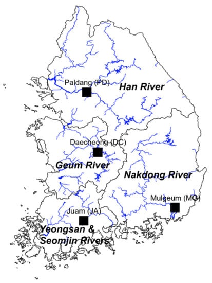
Figure 1.
Water quality monitoring locations at four major rivers in Korea applied to time series prediction models.
In these monitoring stations, water quality data were compiled on a monthly basis from January 2009 to December 2018 through the Water Environment Information System which was maintained by the National Institute of Environmental Research, Korea. Out of a total of 43 water quality parameters observed, we used only 10 water quality variables with relatively few missing values for the given period (Table 1). These included water temperature (°C), pH (-), dissolved oxygen (mg/L), biochemical oxygen demand (BOD, mg/L), chemical oxygen demand (mg/L), suspended solids (mg/L), electrical conductivity (µS/cm), total nitrogen (mg/L), total phosphorus (T-P, mg/L), and total coliforms (cfu/100 mL). Discharge at the closest water quality monitoring stations was taken in the same period from the Water Management Information System operated in the Han River Flood Control Office, Korea. We also collected other relevant record, meteorological data, for the corresponding period, which were available publicly at Open MET Data Portal in the Korea Meteorological Administration. Note that meteorological data adjacent to each water quality monitoring station are aggregated by month using the average (operation) for air temperature, relative humidity, and wind speed as well as using the sum for precipitation and solar radiation. Similarly, the sum aggregate function was used to transform flow rate data from daily to monthly time resolution. Any missing value in discharge was also replaced by imputed values using a linear interpolation approach.

Table 1.
Descriptive statistics of water quality parameters monitored (monthly) at four different monitoring stations (PD, MG, DC, and JA) during the period of 2009 to 2018 (n = the number of data and CV = the coefficient of variation).
2.2. Input Data Preparation
Using all of the data (sources) listed above, various data sets were constructed to test the predictive accuracy of deep learning models. Firstly, we prepared two univariate data sets which included only one target variable. This was conducted because the baseline forecasting method, an autoregressive integrated moving average (ARIMA) model, to be compared to the adopted deep learning models, only accepted a single time series (see Section 2.3). For each performance test of these univariate data sets, either BOD or T-P was selected as the (target) dependent variable. Next, two multivariate data sets consisting of one of two target parameters (e.g., BOD or T-P) as well as the remaining 9 parameters out of 10 observed variables were built not only to examine the performance variation in deep learning models depending on dependent variables, but also to compare their accuracy to that of univariate data sets. Finally, several factors which were capable of affecting model performance were also evaluated by creating three different multivariate data sets. Those data sets were, in particular, developed by increasing the number of important independent variables (from 3 to 9), adjusting sliding window size in multiple input multi-step output (deep learning) models (from 9 through 12 to 15 months for multiple input and from 1 through 2 to 3 months for multi-step output), and incorporating additional variables such as discharge and meteorological data in the given multivariate data sets. Note that square root and log (with a base of 10) transformation are applied to BOD and T-P variables in univariate data sets, respectively, whereas the standardization method (namely, Z-score normalization) is used to make all independent variables, except for dependent variable, on the same scale in multivariate data sets. However, the ARIMA model was fitted to the raw time series data. All decisions of adopting different data preprocessing processes were made by trial and error to maximize the performance of all predictive models tested.
2.3. Applied Prediction Algorithms
We performed benchmark tests on different data sets using various (time series) prediction algorithms (Figure 2). In a series of tests, while the ARIMA played a role as the baseline model, three standalone and one hybrid deep learning algorithms were adopted for performance comparison with the reference ARIMA model. The prediction accuracy for all prediction algorithms is assessed in terms of the mean absolute percentage error (MAPE, in unit of %), which is one of the most common performance measures in time series forecasting. The deep learning algorithms we used were recurrent neural network (RNN), gated recurrent unit (GRU), LSTM, and those combined with CNN and GRU, all of which were widely applied to modern time series data. The chosen architecture of all applied deep learning models, except for the LSTM algorithm which included 2 layers of LSTM cells (namely, a stacked LSTM) as well as the hybrid algorithm which consisted of (1D) convolutional layer, max pooling layer, and GRU layer in series, had a single hidden layer. Note that we only apply a dropout rate of 0.2 and a recurrent dropout rate of 0.2 to the hidden layer in a single GRU algorithm. Moreover, while RNN, GRU and the initial layer of LSTM cells adopted the hyperbolic tangent (namely, tanh) function as non-linear activation, the rectified linear unit (namely, ReLU) function was used in the second layer of LSTM cells as well as convolutional layer in the hybrid algorithm. The root mean squared propagation (namely, RMSprop) was used to improve training speed and performance of all applied deep learning algorithms, where the learning rate and rho were set to 0.001 and 0.9, respectively. The total number of trainable model parameters were 708 for RNN, 415 for GRU, 29,761 for stacked LSTM, and 8,705 for hybrid one. More detailed information on those implemented models such as textual summary and graph plot is documented in the final project report [29].
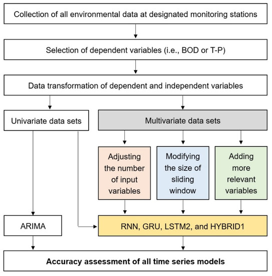
Figure 2.
Schematic diagram illustrating a series of steps used to evaluate all applied time series models, including (input and output) data preparation.
The use of a free statistical software R (Ver. 4.0.4, The R Foundation, Vienna, Austria) as well as RStudio (Ver. 1.3.1073, RStudio, PBC., Boston, MA, USA) allowed us to evaluate the performance of all prediction algorithms, including the ARIMA model. More specifically, we used the forecast package (Ver. 8.13) in R to automatically search the best ARIMA model for the given univariate time series (from the auto.arima function). Different types of deep learning algorithms were also developed and assessed in R using the keras package (Ver. 2.4.0), a high-level deep learning library developed originally for Python, regardless of univariate and multivariate time series. Note that manipulation of time series data is conducted with the zoo package (Ver. 1.8-8). All developed deep learning algorithms were applied on partitioned data sets consisting of 70% of the data for training (n = 84) and the remaining 30% for testing (n = 36). The partitioned data sets were divided again into several equal segments (i.e., multiple samples) using an overlapping sliding (or moving) window with 1 month sliding interval to maximize the amount of data provided to deep learning algorithms. In other words, the windows where 9 and 3 (monthly) time steps were adopted as input and output (in multiple input multi-step output models), respectively, slid by 1 month. In this case, the following window overlapped with the preceding window by 8 (for input) and 2 months (for output). Those deep learning algorithms were trained for 100 epochs with a batch size of 12.
2.4. Variable Selection
Removing irrelevant variables from the data sets assists in not only reducing the execution time of predictive models, but also enhancing their performance. For this study, the selection of important variables (namely, feature selection) was conducted easily with the help of the scikit-learn package, a popular library for machine learning in Python. The criterion for ranking all candidate independent variables we employed was the Pearson correlation coefficient (provided through the f_regression function). Note that the reticulate package (Ver. 1.20) in R enables us to use and run any Python code such as modules, classes, and functions immediately in a R environment. During the tests, the variables to be included in the model increased progressively from 3 to 9 (based on the variable importance determined from the Pearson correlation coefficient).
3. Results and Discussion
3.1. Performance Assessment on Univariate Data Sets
Table 2 presents the performance of all prediction algorithms for two dependent variables (i.e., BOD and TP) at four different monitoring locations (i.e., PD, MG, DC, and JA) using testing data in univariate data sets, in terms of MAPE (%). Note that the accuracy of prediction algorithms for testing data is almost equivalent to or lower than that of training data (not shown here for simplicity). Furthermore, the lower the MAPE is, the better the accuracy of prediction algorithm is. It was found from the table that the ARIMA model recorded higher error rates than four deep learning models (i.e., RNN, GRU, LSTM2, and HYBRID1), regardless of dependent variables as well as monitoring sites. In fact, the ARIMA model results achieved error rates as low as 27.32% for BOD and 27.61% for T-P. In contrast, deep learning models yielded MAPE values in the range of 6.51–18.78% for BOD and 7.98–18.66% for T-P. In addition, the predictive accuracy of the ARIMA model varied widely from station to station as well as from variable to variable. This inconsistent performance of the ARIMA model was similar to the results observed for deep learning models. In summary, even though we do not specify a universal model which works best in any situation, deep learning models lead to better performance the traditional method ARIMA. At this moment, we cannot clearly explain why both ARIMA and deep learning models show heterogeneous (prediction) performance according to stations and dependent variables.
Table 2.
The predictive accuracy of five prediction algorithms (i.e., ARIMA plus four deep learning models) for two targe variables (i.e., BOD and T-P) at four different monitoring stations (PD, MG, DC, and JA) in univariate data sets in terms of MAPE (%).
3.2. Performance Assessment on Multivariate Data Sets
The performance of all prediction algorithms was also assessed against testing data in multivariate data sets, with respect to MAPE (%) (Table 3). Please be aware that the predictive accuracy of four deep learning algorithms is compared to that of the ARIMA model obtained from single dependent variable. From the table, it was observed that deep learning models did not always show superior performance than the ARIMA model. More specifically, although deep learning models provided relatively accurate forecasting of BOD (time series) compared to that of the ARIMA model, their predictive accuracy for T-P significantly decreased depending on algorithms and stations. In fact, MAPE values were highest for HYBRID1 in PD (108.30%), RNN in MG (368.80%), and GRU in DC (121.80%) and JA (243.60%). Taken together, adding more independent (water quality) variables to deep learning models neither necessarily improves the accuracy of prediction nor maintains the performance steadily across stations.
Table 3.
The predictive accuracy of five prediction algorithms (i.e., ARIMA plus four deep learning models) for two target variables (i.e., BOD and T-P) at four different monitoring stations (PD, MG, DC, and JA) in multivariate data sets in terms of MAPE (%).
3.3. Influence of Other Factors on Performance
3.3.1. The Number of Input Variables
Figure 3a,b displays the variation in the performance of a particular deep learning model LSTM2 for BOD and T-P at four monitoring sties in response to the number of (input) variables, respectively. Note that independent variables are added sequentially to the model according to their importance provided by the proposed variable selection approach (see Section 2.4). As can be seen in the figures, MAPE values of the LSTM2 model changed significantly based on the number of input variables, regardless of target variables BOD and T-P. The accuracy of prediction was often improved by incorporating a few variables in the model at some stations (e.g., one more variable for BOD at PD and two more variables for T-P at PD), but its performance fluctuated remarkably among four stations. In some cases, the error rates were further reduced by incorporating the maximum number of variables (i.e., eight parameters), as compared to the minimum number of variables (i.e., three parameters). All these results reveal that determining the optimal number of input variables is a very complex task that inevitably requires an iterative process of searching for the minimal error for a given multivariate data set.
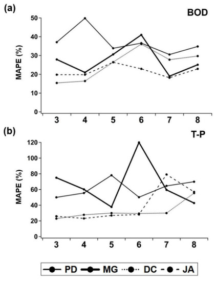
Figure 3.
Changes in MAPE values of the LSTM2 model for (a) BOD and (b) T-P at four monitoring locations according to the number of input variables.
3.3.2. Sliding Window Size
The influence of sliding window size on the accuracy of prediction was also studied in the LSTM2 model at three stations (Table 4). In the table, MAPE values of the LSTM2 model at PD was specifically excluded due to extremely low performance ranging from 105 (ten to the power of five) to 107% (ten to the power of seven). It was determined from the table that either increasing (multiple) input steps from 9 through 12 to 15 months or decreasing multi-step output from 1 through 2 to 3 months did not simply result in the performance improvement of a particular deep learning model. In addition, the predictive accuracy did not increase gradually in accordance with dependent variables as well as stations. Consequently, altering time steps involved in input and output definitely causes the variation in the accuracy of prediction. However, the best performance of a given deep learning algorithm can be achieved through an iterative search for the optimal sliding window size at each station, as discussed in Section 3.3.1.
Table 4.
The predictive accuracy of the LSTM2 algorithm for BOD and T-P based on different input (ranging from 9 through 12 to 15 months) and output steps (ranging from 1 through 2 to 3 months) in terms of MAPE (%).
3.3.3. Relevant Variables
Figure 4a,b illustrates changes in the predictive accuracy of four deep learning models for BOD and T-P at one particular monitoring site DC when more independent variables associated with water quality are added. The relevant variables included additionally in the model were discharge and five different meteorological variables (see Section 2.1). In the figures, individual parameters belonged to the upper category are labeled as W for water quality variables, M for meteorological variables, and D for discharge variable only. The error bars indicate the standard deviation of MAPE values obtained from four deep learning models. It was confirmed from the figure that incorporating both discharge and meteorological variables into deep learning models helped elevate the predictive accuracy of BOD, whereas the reverse is true for T-P. Out of all possible combinations of variables examined, the contribution of discharge variable to reduction in error rates was relatively larger than those of meteorological variables only as well as meteorological plus discharge variables, regardless of the dependent variables.
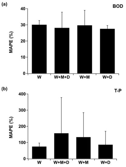
Figure 4.
Changes in MAPE values of four deep learning models for (a) BOD and (b) T-P at one monitoring location DC in response to different multivariate data sets containing water quality variables only (indicated as W), water quality, meteorological, and discharge variables (indicated as W + M + D), water quality and meteorological variables (indicated as W + M), and water quality and discharge variables (indicated as W + D).
4. Conclusions
The intention of this study was to assess the predictive ability of deep learning algorithms for surface water quality in the short term. We constructed and employed three individual and one hybrid algorithms, which were widely adopted for time series prediction, to compare their performance to that of the traditional approach, ARIMA. By providing the modified data sets to all prediction models, the following conclusions were made.
- All deep learning algorithms applied to univariate data sets achieved more reliable forecasts than the ARIMA model whatever the dependent variables BOD and T-P. However, the performance of all prediction models, including ARIMA, was heavily dependent on monitoring stations.
- Using multivariate data sets, we observed noticeable improvement in the predictive accuracy of deep learning models for BOD rather than for T-P (in contrast to that of the ARIMA model derived from each dependent variable). This implied that additional water quality variables did not always enhance the accuracy of prediction for all target variables.
- The number of input variables and sliding window size (input and output steps in the models) were responsible for changes in the performance of deep learning models. The highest prediction accuracy of deep learning models was achieved with the addition of discharge variable (to existing multivariate data sets), instead of using other data sets merging water quality and relevant parameters such as meteorological variables or both meteorological and discharge variables. In our case, this assumption is, however, only valid for prediction of BOD (time series).
- As a preliminary study, this study did not examine the effectiveness of other advanced variants such as encoder-decoder model and attention mechanism, which evolved from traditional deep learning approaches proposed for time series forecasting. More research is, therefore, needed to verify the superiority of those single algorithms, in addition to ensemble learning which combine predictions from multiple (deep learning) models to improve its prediction accuracy over a standalone model. Moreover, as the performance of deep learning algorithms was noticeably affected by the amount of data, model architectures, and dependent variables, these issues should be carefully addressed when developing short-term surface water quality prediction models, specifically using data sets updated monthly or weekly.
Author Contributions
Conceptualization, S.-I.S. and E.J.H.; methodology, S.-I.S. and E.J.H.; formal analysis, S.-I.S. and S.-H.K.; writing—original draft preparation, H.C. and S.J.K.; writing—review and editing, H.C. and S.J.K.; supervision, S.J.K. All authors have read and agreed to the published version of the manuscript.
Funding
This study was supported by a grant (NIER-2020-04-02-129) from the National Institute of Environmental Research (NIER), which was funded by the Ministry of Environment (MOE) of the Republic of Korea.
Conflicts of Interest
The authors declare no conflict of interest.
References
- Than, N.H.; Ly, C.D.; Van Tat, P. The Performance of Classification and Forecasting Dong Nai River Water Quality for Sustainable Water Resources Management Using Neural Network Techniques. J. Hydrol. 2021, 596, 126099. [Google Scholar] [CrossRef]
- Liu, P.; Wang, J.; Sangaiah, A.K.; Xie, Y.; Yin, X. Analysis and Prediction of Water Quality Using LSTM Deep Neural Networks in IoT Environment. Sustainability 2019, 11, 2058. [Google Scholar] [CrossRef] [Green Version]
- Zhi, W.; Feng, D.; Tsai, W.P.; Sterle, G.; Harpold, A.; Shen, C.; Li, L. From Hydrometeorology to River Water Quality: Can a Deep Learning Model Predict Dissolved Oxygen at the Continental Scale? Environ. Sci. Technol. 2021, 55, 2357–2368. [Google Scholar] [CrossRef] [PubMed]
- Lee, S.; Lee, D. Improved Prediction of Harmful Algal Blooms in Four Major South Korea’s Rivers Using Deep Learning Models. Int. J. Environ. Res. Public Health 2018, 15, 1322. [Google Scholar] [CrossRef] [PubMed] [Green Version]
- Peterson, K.T.; Sagan, V.; Sloan, J.J. Deep Learning-Based Water Quality Estimation and Anomaly Detection Using Landsat-8/Sentinel-2 Virtual Constellation and Cloud Computing. GIScience Remote Sens. 2020, 57, 510–525. [Google Scholar] [CrossRef]
- Li, Z.; Ling, K.; Zhou, L.; Zhu, M. Deep Learning Framework with Time Series Analysis Methods for Runoff Prediction. Water 2021, 13, 575. [Google Scholar]
- Udayakumar, K.; Subiramaniyam, N.P. Deep Learning-Based Production Assists Water Quality Warning System for Reverse Osmosis Plants. H2Open J. 2020, 3, 538–553. [Google Scholar]
- Barzegar, R.; Aalami, M.T.; Adamowski, J. Short-Term Water Quality Variable Prediction Using a Hybrid CNN–LSTM Deep Learning Model. Stoch. Environ. Res. Risk Assess. 2020, 34, 415–433. [Google Scholar] [CrossRef]
- Yan, J.; Liu, J.; Yu, Y.; Xu, H. Water Quality Prediction in the Luan River Based on 1-Drcnn and Bigru Hybrid Neural Network Model. Water 2021, 13, 1273. [Google Scholar]
- Thai-Nghe, N.; Thanh-Hai, N.; Ngon, N.C. Deep Learning Approach for Forecasting Water Quality in IoT Systems. Int. J. Adv. Comput. Sci. Appl. 2020, 11, 686–693. [Google Scholar]
- Wang, X.; Zhang, C. Water Quality Prediction of San Francisco Bay Based on Deep Learning. J. Jilin Univ. (Earth Sci. Ed.) 2021, 51, 222–230. [Google Scholar]
- Chandra, R.; Goyal, S.; Gupta, R. Evaluation of Deep Learning Models for Multi-Step Ahead Time Series Prediction. IEEE Access 2021, 9, 83105–83123. [Google Scholar]
- Sha, J.; Li, X.; Zhang, M.; Wang, Z.L. Comparison of Forecasting Models for Real-time Monitoring of Water Quality Parameters Based on Hybrid Deep Learning Neural Networks. Water 2021, 13, 1547. [Google Scholar] [CrossRef]
- Baek, S.S.; Pyo, J.; Chun, J.A. Prediction of Water Level and Water Quality Using a CNN-LSTM Combined Deep Learning Approach. Water 2020, 12, 3399. [Google Scholar] [CrossRef]
- Yan, J.; Gao, Y.; Yu, Y.; Xu, H.; Xu, Z. A Prediction Model Based on Deep Belief Network and Least Squares SVR Applied to Cross-Section Water Quality. Water 2020, 12, 1929. [Google Scholar]
- Hu, Z.; Zhang, Y.; Zhao, Y.; Xie, M.; Zhong, J.; Tu, Z.; Liu, J. A water quality prediction method based on the deep LSTM network considering correlation in smart mariculture. Sensors 2019, 19, 1420. [Google Scholar] [CrossRef] [Green Version]
- Faruk, D.Ö. A Hybrid Neural Network and ARIMA Model for Water Quality Time Series Prediction. Eng. Appl. Artif. Intell. 2010, 23, 586–594. [Google Scholar]
- Li, Z.; Peng, F.; Niu, B.; Li, G.; Wu, J.; Miao, Z. Water quality prediction model combining sparse auto-encoder and LSTM network. IFAC-Pap. 2018, 51, 831–836. [Google Scholar] [CrossRef]
- Zhou, Y. Real-Time Probabilistic Forecasting of River Water Quality under Data Missing Situation: Deep Learning plus Post-Processing Techniques. J. Hydrol. 2020, 589, 125164. [Google Scholar]
- Loc, H.H.; Do, Q.H.; Cokro, A.A.; Irvine, K.N. Deep Neural Network Analyses of Water Quality Time Series Associated with Water Sensitive Urban Design (WSUD) Features. J. Appl. Water Eng. Res. 2020, 8, 313–332. [Google Scholar]
- Najafzadeh, M. Evaluation of conjugate depths of hydraulic jump in circular pipes using evolutionary computing. Soft Comput. 2019, 23, 13375–13391. [Google Scholar] [CrossRef]
- Saberi-Movahed, F.; Najafzadeh, M.; Mehrpooya, A. Receiving more accurate predictions for longitudinal dispersion coefficients in water pipelines: Training group method of data handling using extreme learning machine conceptions. Water Resour. Manag. 2020, 34, 529–561. [Google Scholar] [CrossRef]
- Najafzadeh, M.; Ghaemi, A.; Emamgholizadeh, S. Prediction of water quality parameters using evolutionary computing-based formulations. Int. J. Environ. Sci. Technol. 2019, 16, 6377–6396. [Google Scholar] [CrossRef]
- Najafzadeh, M.; Homaei, F.; Farhadi, H. Reliability assessment of water quality index based on guidelines of national sanitation foundation in natural streams: Integration of remote sensing and data-driven models. Artif. Intell. Rev. 2021, 54, 4619–4651. [Google Scholar] [CrossRef]
- Heddam, S.; Kisi, O. Modelling daily dissolved oxygen concentration using least square support vector machine, multivariate adaptive regression splines and M5 model tree. J. Hydrol. 2018, 559, 499–509. [Google Scholar] [CrossRef]
- Najafzadeh, M.; Niazmardi, S. A Novel Multiple-Kernel Support Vector Regression Algorithm for Estimation of Water Quality Parameters. Nat. Resour. Res. 2021, 30, 3761–3775. [Google Scholar] [CrossRef]
- Zhou, J.; Wang, Y.; Xiao, F.; Wang, Y.; Sun, L. Water quality prediction method based on IGRA and LSTM. Water 2018, 10, 1148. [Google Scholar] [CrossRef] [Green Version]
- Khullar, S.; Singh, N. Water quality assessment of a river using deep learning Bi-LSTM methodology: Forecasting and validation. Environ. Sci. Pollut. Res. 2021. [Google Scholar] [CrossRef]
- Korea Water Resources Association. A Study on Water Quality Assessment with Data-Driven Models and Its Short-Term Prediction Methods; National Institute of Environmental Research: Incheon, Korea, 2021. [Google Scholar]
Publisher’s Note: MDPI stays neutral with regard to jurisdictional claims in published maps and institutional affiliations. |
© 2021 by the authors. Licensee MDPI, Basel, Switzerland. This article is an open access article distributed under the terms and conditions of the Creative Commons Attribution (CC BY) license (https://creativecommons.org/licenses/by/4.0/).