Field Quality Control of Spectral Solar Irradiance Measurements by Comparison with Broadband Measurements

Abstract

Measurement of solar spectral irradiance is required in an increasingly wide variety of technical applications, such as atmospheric studies, health, and solar energy, among others. The solar spectral irradiance at ground level has a strong dependence on many atmospheric parameters. In addition, spectroradiometer optics and detectors have high sensitivity. Because of this, it is necessary to compare with a reference instrumentation or light source to verify the quality of measurements. A simple and realistic test for validating solar spectral irradiance measurements is presented in this study. This methodology is applicable for a specific spectral range inside the broadband range from 280 to 4000 nm under cloudless sky conditions. The method compares solar spectral irradiance measurements with both predictions of clear-sky solar spectral irradiance and measurements of broadband instruments such as pyrheliometers. For the spectral estimation, a free atmospheric transmittance simulation code with the air mass calculation as the mean parameter was used. The spectral direct normal irradiance ($G_{b\lambda }$) measurements of two different spectroradiometers were tested at Plataforma Solar de Almería, Spain. The results are presented in this article. Although only $G_{b\lambda }$ measurements were considered in this study, the same methodology can be applied to the other solar irradiance components.

1. Introduction

Ninety-seven percent of the radiation incident on the top of Earth’s atmosphere coming from the Sun is distributed between the wavelengths: 290 to 3000 nm [1]. The distribution of radiation within this wavelength range is known as the solar radiation. As solar radiation travels from the outer layers through the atmosphere to the ground, the solar spectrum is attenuated and shaped due to absorption and scattering processes. These extinction processes result from the interaction between the radiation and the atmosphere components, such as aerosols, water, and gas molecules, showing a strong spectral dependence. The intensity with which these phenomena affect solar radiation depends on the number of interactions. The shape of the solar spectrum thus depends on the length of the light path through the atmosphere and the concentration and nature of its components. As a result, the spectral distribution of solar radiation varies over time depending on local environment conditions and the Sun’s position [2,3,4,5].

In this sense, the beam irradiance received at ground level by a surface normal to the Sun’s rays, also called spectral beam normal irradiance ($G_{b\lambda })$ or spectral direct normal irradiance ($DN{I}_{\lambda }$), at wavelength $\lambda$ is given by [6]:

$$G_{b\lambda }=G_{0\lambda } T_{R\lambda } T_{o\lambda } T_{n\lambda } T_{g\lambda } T_{w\lambda } T_{a\lambda }=G_{0\lambda } {\displaystyle \prod }_i{T}_{i\lambda }$$

(1)

where $G_{0\lambda }$is the extra-terrestrial spectral irradiance, i.e., the spectral solar irradiance at the atmosphere outer boundary considering the Sun–Earth distance. The $T_{i\lambda }$ factors represent the transmittances due to the different extinction processes considered: Rayleigh scattering ($T_{R\lambda }$), absorption by ozone$(T_{o\lambda })$, NO₂ ($T_{n\lambda }$), uniformly mixed gases ($T_{g\lambda }$) and water vapour ($T_{w\lambda }$), and, finally, aerosol extinction ($T_{a\lambda }$).

According to the Lambert–Beer–Bouguer law, $T_{i\lambda }$ can be expressed as follows.

$$T_{i\lambda }=e^{-m {\tau }_{i\lambda }}$$

(2)

where ${\tau }_{i\lambda }$ is the optical thickness associated to the i-extinction process, which gives an idea of how transparent a medium is. The atmospheric components are distributed along the atmospheric column differently. Although in Equation (2) the optical air mass, $m$, should be calculated for each atmospheric constituent, the calculation of m according to the Kasten and Young formula [7] can be adopted in a simplified way. For a more detailed definition of air mass, see the SMARTS report [6]. The Kasten and Young formula allows the calculation of the m corrected with the pressure values [7] as follows:

$$\mathrm{m} \equiv \frac{1}{\sin \alpha +0.50572 {(6.07995+\alpha )}^{-1.6364}} \frac{p}{p_0}$$

(3)

The solar elevation $\alpha$ is calculated by using formulas in the bibliography as a function of the local geographic coordinates and time [1,8]. In Equation (3), $p$ is the pressure, in (kPa), and $p_0$ is the reference pressure at standard conditions, 101.325 kPa. Their quotient can be used to correct the calculation of $\mathrm{m}$ for local conditions, especially at elevated locations with significantly lower atmospheric pressure.

The knowledge of the amount of radiation that achieves ground level per wavelength has become an important issue in such different disciplines as the atmospheric sciences, biology, medicine, agriculture, materials sciences, and solar energy technologies.

On the one hand, there are many tools to estimate the spectral solar radiation at ground level in terms of given atmospheric parameters. For example, there are atmospheric radiative transfer models such as libRadtran [9], MODTRAN [10], and LOWTRAN [11] that solve the equation for radiative transfer in the different atmospheric layers. However, there are also atmospheric spectral transmittance models, such as SMARTS [6,12], which use correlations to accurately approximate the calculation of transmittances based on the abundance of each atmospheric component and the spectral absorption coefficients of the absorbers. These codes are good enough to give an idea of what the spectral solar radiation at ground level should be, but they require a set of inputs that are often hard to know.

On the other hand, spectroradiometers measure spectral irradiance, which is the radiant flux (power) received by a surface per unit area and unit wavelength. In this article, we express it in units of watts per square meter per nanometer (W m⁻² nm⁻¹).

Spectroradiometers consist of an optical system and sensors. The optical system, called a spectrometer, separates radiation according to its wavelength for a given spectral range. The calibrated sensor measures the irradiance of the radiation incident on it for the selected wavelength. The commercial spectroradiometers, which commonly can be found, may be divided by their principle of operation into three important groups [13]:

• Spectroradiometers with a monochromator, which usually utilize a rotating diffraction grating. The rotating grating selects the wavelength to be displayed on a single sensor, e.g., a photomultiplier (PMT) or photodiode according to the wavelength to measure. Because of the operation procedure, they expend some minutes to take the measurements for a specific spectral range. The time necessary to complete a whole scan depends upon both the wavelength resolution and the spectral range of measurement, e.g., 10 min for some types of conventional high-quality spectroradiometers [1].
• Spectroradiometers with a fixed grating that projects the spectrum on a detector array, usually a photodiode or charge-coupled detector (CCD) array. No moving components are used in this category of spectroradiometers. They are faster-measuring because they measure the spectral irradiance at each wavelength at the same time. However, their measurements generally have a lower quality than the measurements taken with the other kind of spectroradiometers.
• A third class of spectroradiometers based on a Fourier transform can be found. They use a Michelson interferometer to measure how the signal of the interference oscillates by varying the path length travelled by light between two mirrors. The intensity of the spectrum is obtained with a further digital procedure. This class of spectroradiometers achieves the highest spectral resolution and allows the measurement of far-infrared spectra. This class of spectroradiometers was not considered in the present study.

There is a compromise between accuracy and measurement time. A shorter measurement time for each scan implies more scans can be averaged during a fixed sample analysis time [14]. However, the spectroradiometers with monochromators are usually slower and use high-precision sensors that make them the favorable for accurate measurements. In addition, the use of coolers in both cases, for instance, based on Peltier cells, helps to reduce the thermal noise, which is a background noise signal that appears because of sensor heating.

Inter-comparisons [15] between spectroradiometers with the same characteristics, or the comparison with calibrated lamps, can be made to know the state of the instrumentation. Other self-checking features are now available with monitoring instruments. These tests provide the operator with information on the stability of the instrument, for example, by checking the operation of the PMT and the analogue-to-digital conversion or determining whether the optics of the instrument are working properly [1].

To analyze large spectral databases in an automated way, Jesús Polo et al. [16] proposed to evaluate the average photon energy (APE) of each spectrum. The method consisted of calculating the APE value of the measured spectrum and comparing it with the APE value of the spectrum calculated with SMARTS for clear days. If the APE was 1.5 times higher than the clear-sky APE, the spectrum was discarded. More recently, G. Nofuentes et al. have proposed the spectral index to replace the APE [17].

Other validation methods are used to validate spectral simulations with ground measurements [18,19,20,21]. These methods can be implemented in both directions, to validate models or measurements, provided that the needed data to run the models are available.

However, it is often difficult to find available data or instrumentation to validate spectral measurements. This article, based on a previous study [22], reports on a new method for the quality control (QC) of spectral direct normal irradiance measurements, $G_{b\lambda }$, under cloudless sky conditions. This simple method is based on the use of an atmospheric radiative transfer code, considering only the air mass calculation, $m$, and broadband radiometers, in this case, a pyrheliometer for the spectral direct normal irradiance solar radiation component validation. This methodology facilitates the application of QC in most locations where spectral solar irradiance measurements are performed.

2. Materials and Methods

2.1. Instrumentation and Atmospheric Radiative Transfer Codes

The Plataforma Solar de Almería (PSA) site is in southeast Spain. It is the largest European research, development, and test center devoted to solar concentration technologies. It has had a meteorological station since 1988, primarily for measuring broadband solar radiation (global, direct, and diffuse radiation) but also for other generic weather variables. Thanks to the collaboration between Centro de Investigaciones Energéticas, Medioambientales y Tecnológicas (CIEMAT) and the Deutsches Zentrums für Luft- und Raumfahrt (DLR), the facilities of the new weather station for solar technologies Meteorological Station for Solar Technologies (METAS) were inaugurated in June 2013 [23]. It is a joint facility that aims at the development of activities related to measurement and characterization of solar radiation for energy applications.

For this study, two spectroradiometers were placed at METAS.

The first one, Spec1, is the SPECTRO320 D manufactured by Instruments Systems. It uses a double monochromator and incorporates a PMT and a lead sulphur detector (PbS), for both 190–1050 nm and 800–2500 nm spectral ranges, respectively. The sensors are cooled by the Peltier effect. It measures the solar $G_{b\lambda }$ by using a probe mounted in a solar tracker. For the $G_{b\lambda }$ measurement, the instrument takes 9 min and 45 s. The spectroradiometer is calibrated by international centers, using a deuterium light source for the UV spectral range and a halogen light source for the VIS/NIR spectral range [24,25].

The second instrument, Spec2, is composed of two spectroradiometers operating in different spectral ranges and is the AvaSpec-NIR1.7/3648-USB2-RM developed by Avantes. Both spectroradiometers are based on a symmetrical Czerny–Turner design. To record the spectral distribution of the solar radiation over the 200–1110 nm spectral range, it uses a 3648-pixel CCD detector array. For the 900–1750 nm spectral range, it uses an InGaAs detector with 256 pixels. This configuration allows measuring the $G_{b\lambda }$ in the order of milliseconds, allowing several measurements to be taken and averaged over a short time interval.

Both spectroradiometers have time synchronization to work simultaneously, and they are regularly calibrated by using standard traceable lamps. For the shortwave spectral range calibration, a deuterium–halogen lamp may be used in either a deuterium–halogen or halogen configuration. The longwave sensor is calibrated by using a Wolfram halogen lamp.

The broadband direct normal irradiance ($G_b$) is measured with a Kipp & Zonen CHP1 pyrheliometer at METAS. The CHP1 is a first-class normal incidence pyrheliometer and complies with the most current ISO and WMO. The CHP 1 is calibrated upon manufacture and is supplied standard with a world radiometric reference (WRR) traceable calibration certificate. It works in the spectral range from 280 to 4000 nm with an expected uncertainty of ±1% [26].

The simple model of the atmospheric radiative transfer of sunshine (SMARTS) [6,12] is used to calculate the solar spectrum at ground level. It computes clear-sky spectral irradiances within the 280–4000 nm spectral range, completely covering the spectral range of broadband instrumentation. The power confined in this spectral range represents 101% of the solar radiation, in comparison with the solar radiation spectral range, 300–2500 nm, as it is defined in [27]. The SMARTS code allows estimating the $G_{b\lambda }$ in terms of parameters such as air mass, ozone, and humidity, among others.

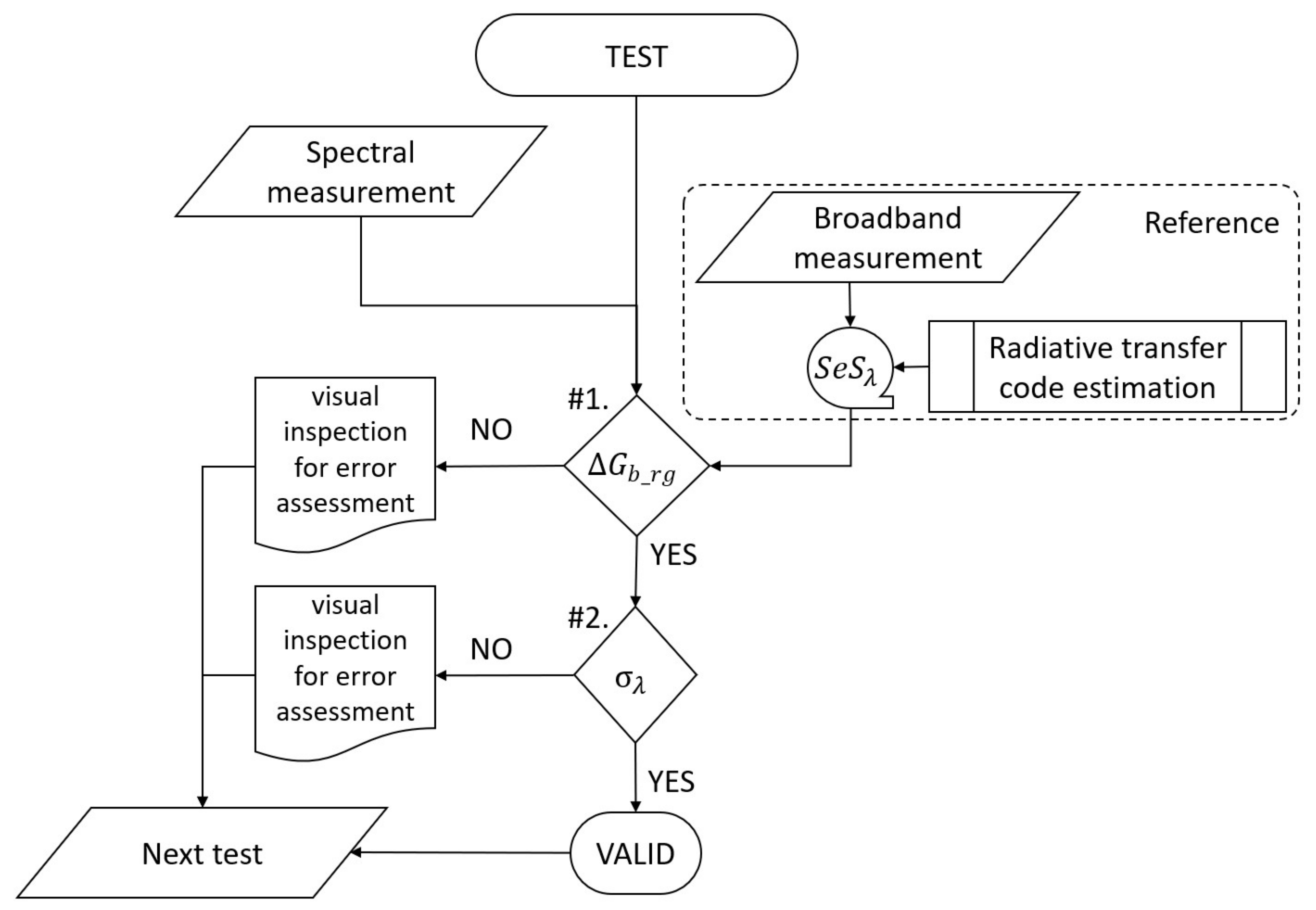
2.2. Quality Control Methodology Description

The spectral irradiance, $DN{I}_{\lambda }$, is related with broadband irradiance, $DNI$, according to the following expression:

$$G_b={{\displaystyle \int }}_a^b{G}_{b\lambda } d\lambda$$

(4)

where a and b are the integration limits for a defined spectral range, e.g., the spectral range of measurement of an instrument. Accordingly, spectral measurements can be compared with broadband measurements. Under these conditions, the comparison does not contemplate the spectral nature of the measurement, but this issue is addressed below. Two basic considerations need to be considered at this stage: the solar irradiance measured with both instruments must be under the same viewing angle, and both spectral and broadband measurements need to be compared within the same spectral range (a, b).

In general, broadband instruments measure solar irradiance over a wider spectral range than spectroradiometers. Consequently, it is necessary to discard the portion of irradiance corresponding to non-common wavelengths to make a proper comparison. This task is not trivial, but atmospheric radiative transfer codes can help in this regard.

Atmospheric radiative transfer codes, such as SMARTS [6,12], estimate the spectral distribution of solar irradiance from local atmospheric and astronomical input parameters. As expressed in Equation (4), both spectral and broadband irradiances are related to each other and, therefore, depend on the same local parameters, as those shown in Equation (1). This fact has led to studies focused on obtaining, for example, aerosol information such as aerosol optical depth or turbidity, from broadband measurements and radiative transfer models [28,29,30,31,32,33].

In this study, the SMARTS code was used to estimate the spectral distribution of the broadband solar irradiance and to help exclude the undesirable part of it. To obtain the spectral distribution of the $G_b$ broadband measurement, the estimated spectral irradiance curve was normalized to the broadband irradiance measurement, resulting in a semi-empirical solar spectrum ($Se{S}_{\lambda }$). For the $Se{S}_{\lambda }$ calculation, the first step was to estimate a spectral irradiance with the radiative transfer model, $G_{b\lambda }^e$. The second step was to normalize this estimation to the value of the broadband measurement, $G_b^m$, according to Equation (5), obtaining the $Se{S}_{\lambda }$ (see Figure 1).

$$Se{S}_{\lambda }=\frac{G_{b\lambda }^e}{{{\displaystyle \int }}_a^b{G}_{b\lambda }^e d\lambda }·G_b^m$$

(5)

where $a$ and $b$ are the wavelength that define the limits of the spectral range of work of the broadband instrumentation, from 280 to 4000 nm in this case.

Once the $Se{S}_{\lambda }$ was calculated, the comparison was possible in two steps (see Figure 2).

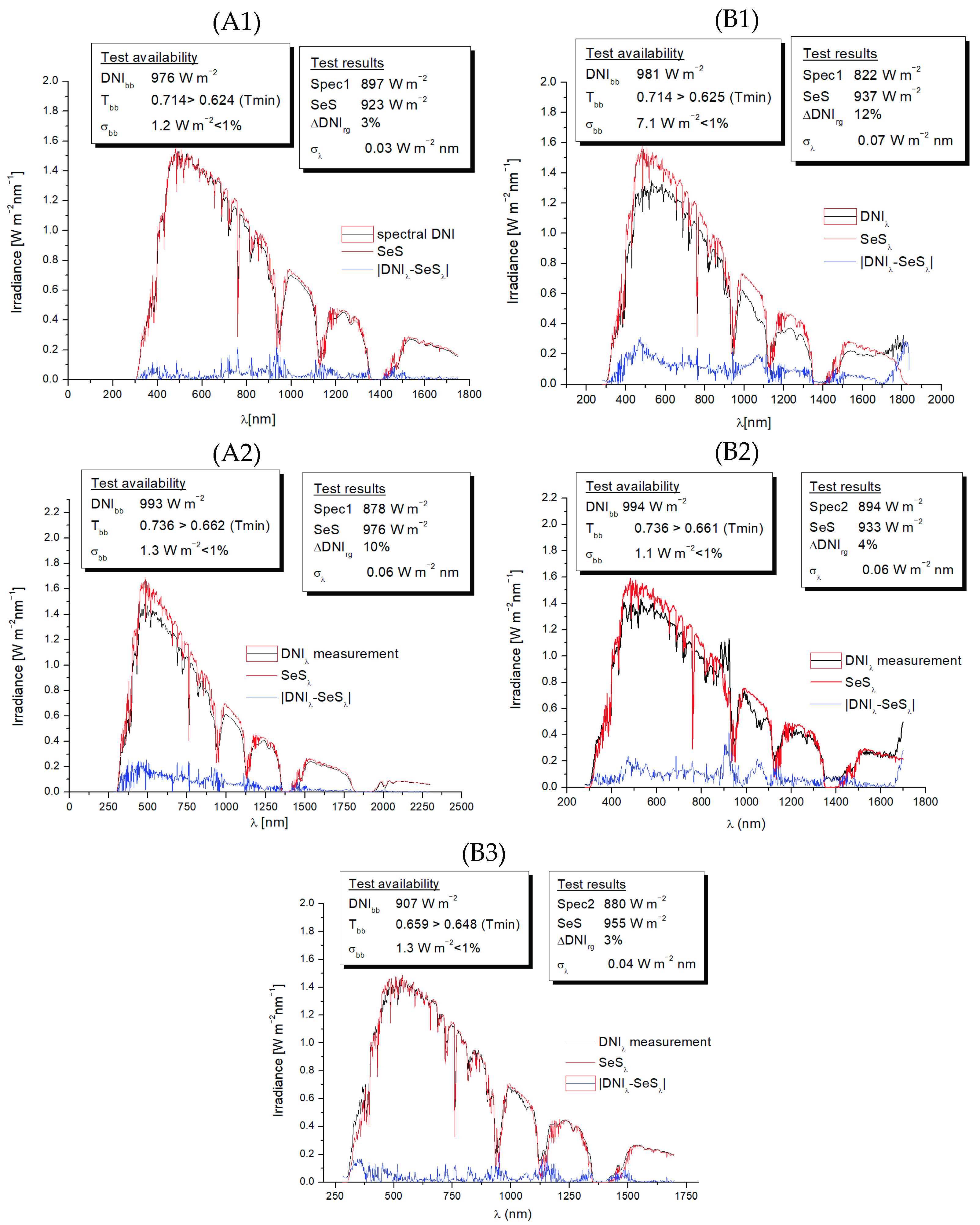
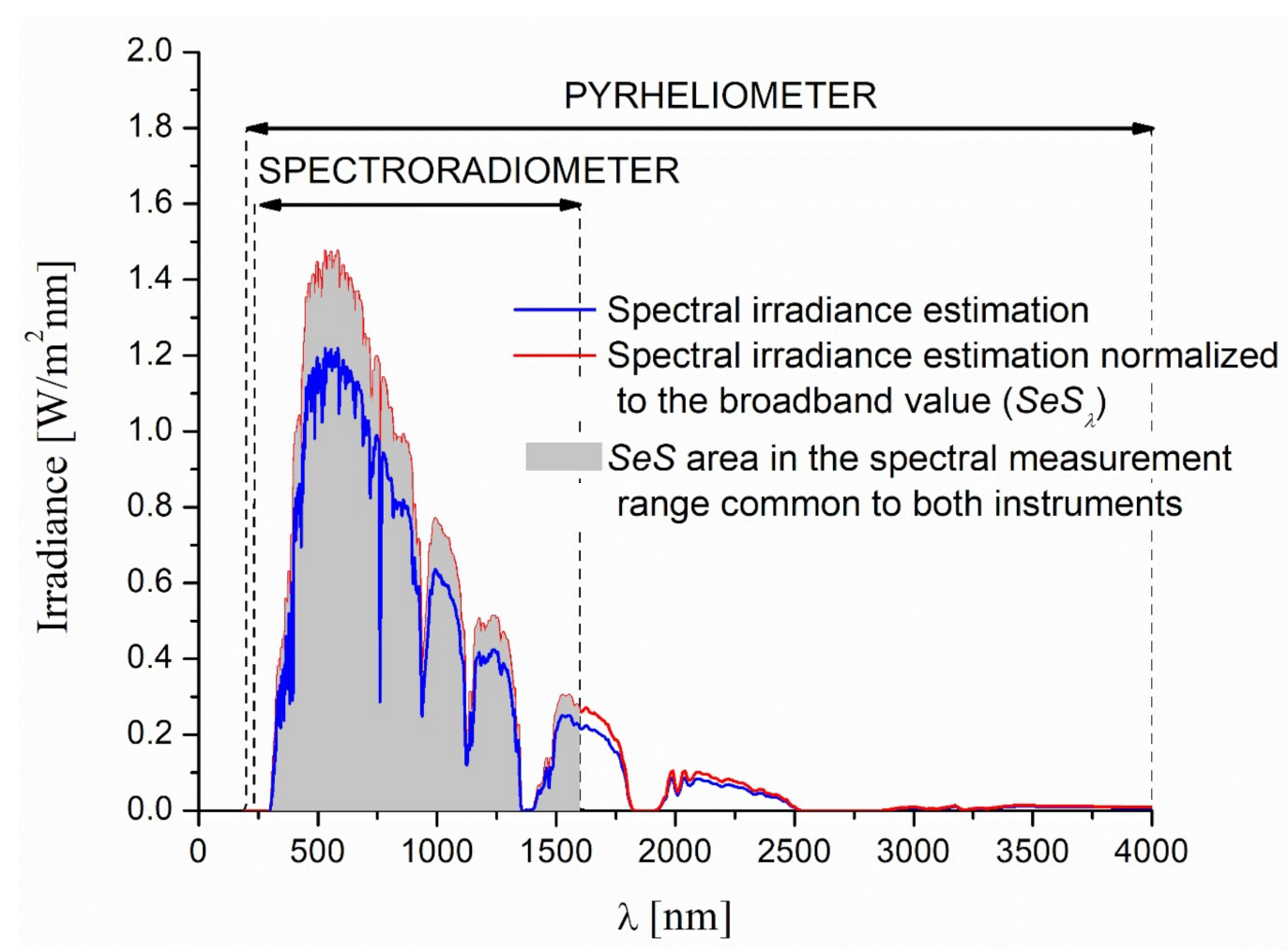
• Calculate the relative error between values of the integral of both the spectral measurement, $G_{b\lambda }^m$, and the $Se{S}_{\lambda }$ for the same spectral range.

  $$\mathsf{\Delta }{G}_{b\_rg}=\frac{{{\displaystyle \int }}_a^{b}Se{S}_{\lambda } d\lambda -{{\displaystyle \int }}_a^b{G}_{b\lambda }^m d\lambda }{{{\displaystyle \int }}_a^{b}Se{S}_{\lambda } d\lambda }·100\%$$

  (6)

  where $\mathsf{\Delta }{G}_{b\_rg}$ is the relative error for the spectral range defined by the operating limits of the spectroradiometer or the spectral range of interest for the validation, $a$ and $b$.
• A comparison of the shape of the two spectra on a graph by calculating the standard deviation,${ \mathsf{\sigma }}_{\lambda }$, of the subtraction of the two spectra, $\left(G_{b\lambda }^m-Se{S}_{\lambda }\right)$, and, if needed, by visual inspection.

  $${\mathsf{\sigma }}_{\lambda }=\sqrt{\frac{{{\displaystyle \sum }}_{i=a}^b{\left[{\left|G_{b\lambda }^m-Se{S}_{\lambda }\right|}_i-\overline{\left|G_{b\lambda }^m-Se{S}_{\lambda }\right|}\right]}^2}{\mathrm{N}-1}}$$

  (7)

  where N is the number of wavelengths ($i$) at which the sample has been measured.

There are causes that can affect the measurement with spectroradiometers related to the handling of the instrument, such as thermal noise or dirt in the optical system, which can be solved by taking appropriate care in the operation of the instrument. However, there are two types of errors that are a consequence of a need for calibration: the one related to the irradiance levels and the one related to the wavelength value at which it is measured.

In this sense, the first step of the proposed methodology compares the irradiance levels in the broadband term (W m⁻²) with the reference instrument, a pyrheliometer, for the whole integration spectral range. At this stage, the relative error resulting from the comparison must be lower than the threshold calculated in Section 3 (Equation (9)).

The second step is to identify errors due to the miscalibration of the optical system on the wavelengths but also errors that may be undetected in the first step. For example, the occurrence of an unwanted peak at a given bandwidth can compensate for a deficiency in the measurement of spectral irradiance at other wavelengths. These are two errors that, when added together, can be missed in the first step of the comparison.

As mentioned above, broadband and narrowband measurements are affected by the same atmospheric parameters. The present methodology is based on the normalization of the estimated spectrum with atmospheric transmittance codes to the broadband measured values. For this reason, under normal sky conditions, most of the inputs for the simulation of the atmospheric conditions and the calculation of the local spectrum can be neglected, if the estimation remains within the confidence margins. However, the definition of the normal sky conditions under which the test can be performed and the calculation of the airmass are still necessary. To support this hypothesis, a sensitivity study is presented in the next section.

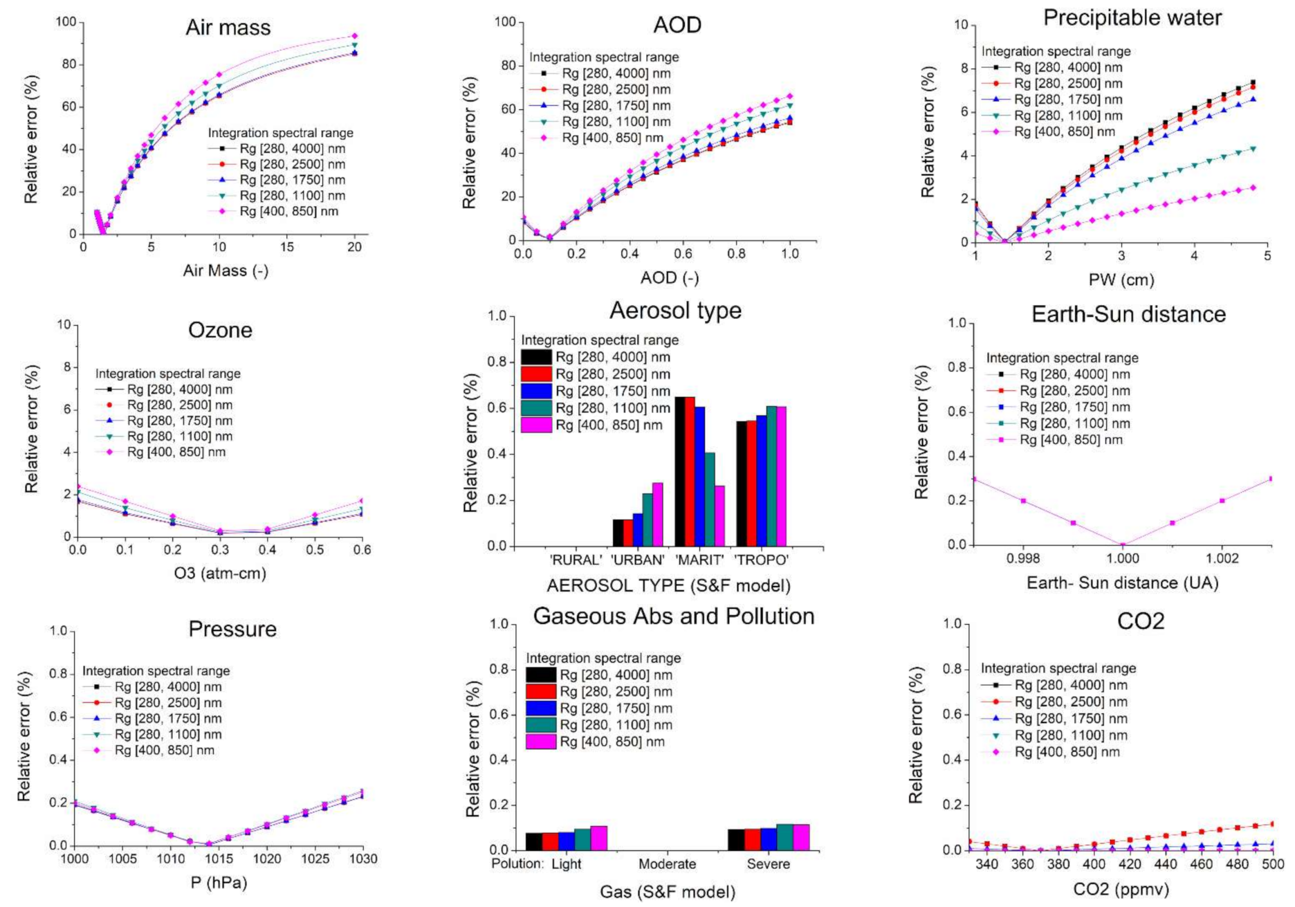
2.3. Sensitivity Analysis Description

A sensitivity analysis was carried out to determine the impact of each SMARTS input on the integral value of the solar spectral irradiance, i.e., on the broadband values. The study considered the usual working spectral ranges of commercial spectroradiometers. The analysis allowed us to discard input parameters that were not necessary to use in the methodology, while maintaining confidence margins under certain sky conditions. The sensitivity analysis was developed by varying each input parameter with respect to the value described in the G173 standard [19,34] (see

Table 1. Parameters, units, values, and steps considered for sensitivity analysis. The atmosphere model considered is the one defined in the U.S. Standard Atmosphere 1976 [34]. The extraterrestrial spectrum is defined in Gueymard (2004) [19].

Variable	Units	Values
		Minimum	Reference	Maximum		No Steps
Site pressure (At 505 masl) a	mb	1000 a	1013.25	1030 a		16
Water vapor	cm	1	3	4.8		20
Ozone (at sea level)	atm-cm	0	0.3	0.6		21
Gaseous Abs and pollution b	--	Severe Pollution b	Moderate Pollution b	Light Pollution b		3
CO2	ppmv	330	370	500		18
Aerosol model b	--	Maritime	Rural	Tropospheric	Urban	4
Atmosphere turbidity (AOD at 500 nm)	--	0	0.084	1		21
Albedo	--	0	0.2	1		10
Earth–Sun distance	AU	0.997	1.0	1.003 a		7
Solar constant, G0	W m−2	1367	1367	1367		1
Air mass		1	1.5	20		25

^a Extreme values at sea level are considered; ^b different atmosphere conditions given by SMARTS code. Detailed descriptions about atmospheric conditions in [19].

). The variation of each parameter was performed considering a wide range of values. This allowed us to see how they influence the irradiance broadband values. In total, 144 different atmosphere conditions were considered to estimate the solar spectra needed to perform the sensitivity analysis.

According to the Equation (1) and the validation method described in this article, the object function for this analysis is:

$$G_{b\_\mathit{rg}}={{\displaystyle \int }}_a^b{G}_{b\lambda }\left(p, w, O_3, g, C{O}_2, aerosols,m\right)d\lambda$$

(8)

where $G_{b\lambda }$ is the spectral direct normal irradiance in (W m⁻² nm⁻¹), $G_{b\_\mathit{rg}}$ is the direct normal irradiance for a specific spectral range in (W m⁻²), and the sub index $rg$ indicates that $G_b$ is calculated for a spectral range from $a$ to $b$ wavelengths in (nm).

The integration spectral ranges, $a$ and $b$, were selected as close as possible to the common spectral range of work of commercial spectroradiometers and broadband instrumentation. Five spectral ranges were considered for the study: 280–4000 nm, 280–2500 nm, 280–1750 nm, 280–1100 nm, and 400–850 nm.

To quantify the weight of each input in the broadband value of the solar radiation for the different spectral ranges, the relative error induced by varying the input with respect to the conditions defined in the standard was calculated, leaving the rest of the inputs unchanged, as indicated in the following equation:

$$\Delta G_{b\_rg}=\left|\frac{G_{b\_rg}^{Ref}-G_{b\_rg}^i}{G_{b\_rg}^{Ref}}\right| \ast 100\%$$

(9)

where $G_{b\_rg}^{Ref}$ is the $G_{b\_rg}$ value given for the standard conditions for the spectral range of interest, and $G_{b\_rg}^i$ is the value of the $G_{b\_rg}$ varying the parameter I for the same spectral range.

The results of the sensitivity analysis calculations were also used to determine the conditions under which the QC methodology could be applied. The results of both the sensitivity analysis and the definition of the times to apply the quality control are included in Section 3.1.

3. Results

3.1. Selection of Inputs and Times to Apply the QC

3.1.1. Sensitivity Analysis

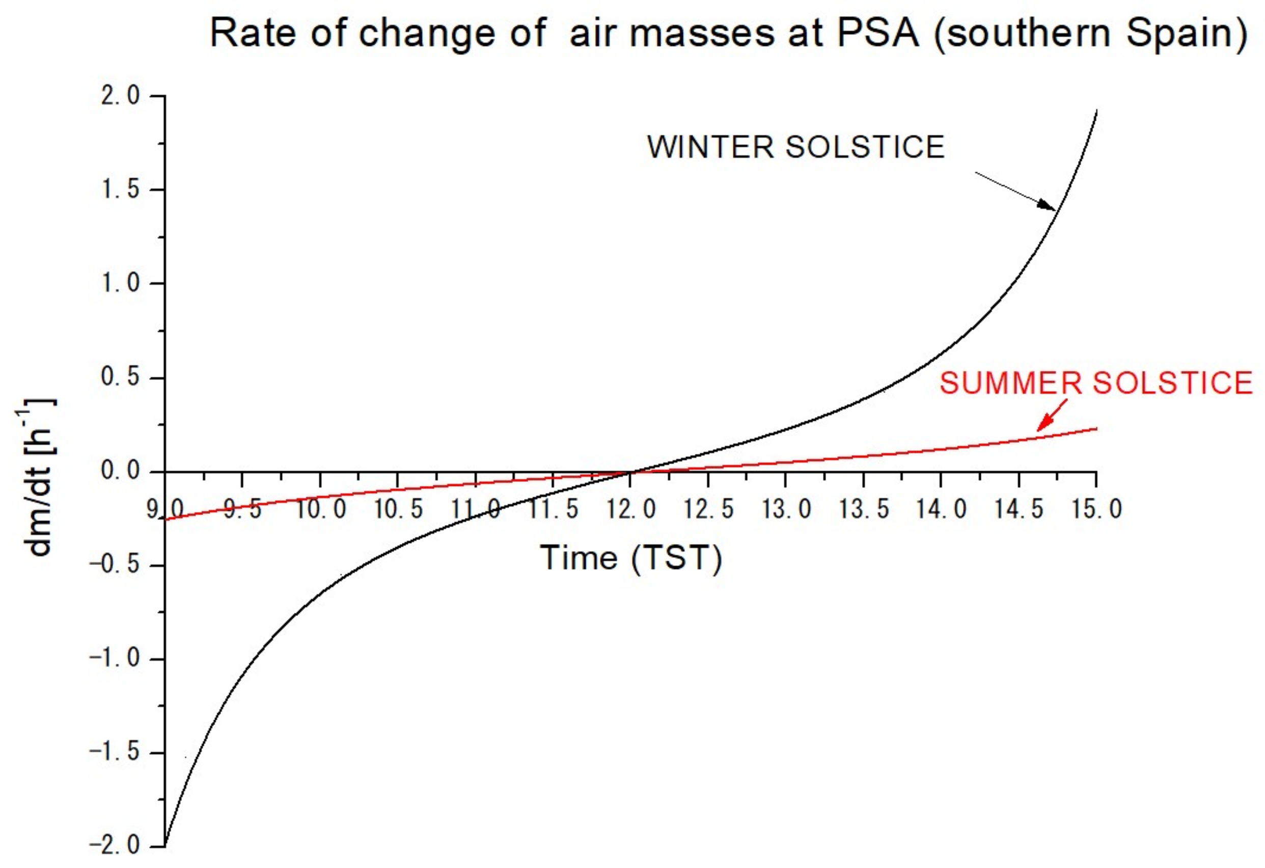
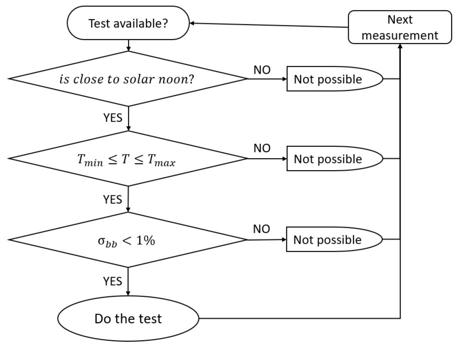
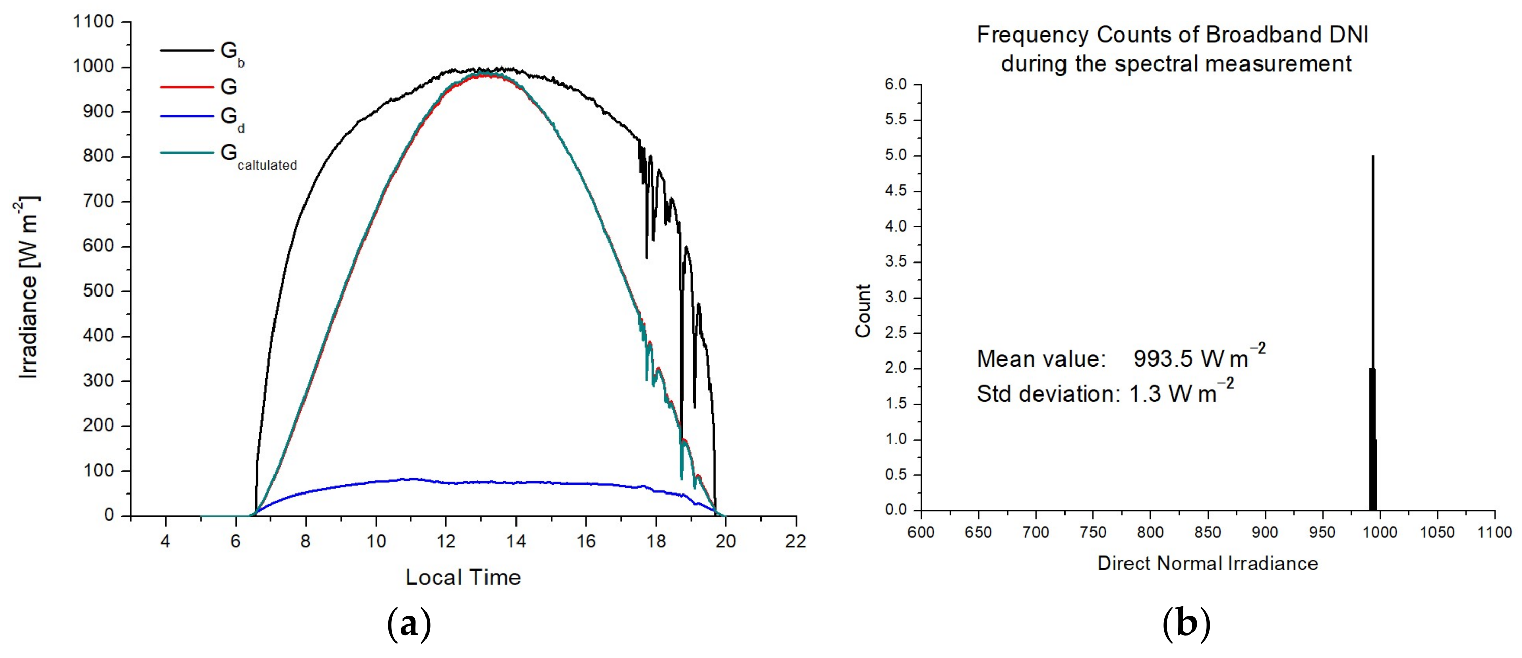
The results of the sensitivity analysis calculation are shown in Figure 3.

Figure 3 shows the results of the calculation of the relative error induced by the variation of each input with respect to the conditions defined in the standard, $\Delta G_{b\_rg}$. As it is shown in the figure, the parameter with the greatest influence was the air mass, $m$, followed by aerosol optical depth (AOD), the precipitable water vapour, the ozone, and the aerosol type. The influence of the rest of the parameters was insignificant in terms of broadband values less than 0.3%. This result highlights both the importance of an accurate m calculation and the choice of a time to measure in which the m variation is negligible, e.g., at solar noon. This is especially important if the time taken by the spectroradiometer is long enough for the measurement to occur under different airmass conditions, as shown at the end of this section.

Figure 3 also shows how the parameters are affected differently depending on the spectral range of integration (colors). This behavior coincides with the fact that the atmospheric transmittance due to each parameter has a spectral dependence. Thus, for example, it was observed that $m$, AOD, and ozone had a greater influence in narrower ranges close to short wavelengths, while precipitable water had a greater influence in ranges containing more wavelengths in the infrared range, as expected.

However, these results are not relevant to the methodology presented. The $\Delta G_{b\_rg}$ values, due to the spectral range of integration, were negligible compared to the variations of the value of each parameter with respect to the standard, as shown in

Table 2. Relative errors according to the spectral range of integration due to a 10% variation of all inputs except m.

SPECTRAL RANGE	(280–4000)	(280–2500)	(280–1750)	(280–1150)	(400–850)
$\Delta {\mathit{G}}_{\mathit{b}\_\mathit{r}\mathit{g}}$	2.80%	2.78%	2.75%	2.84%	2.77%

below. Table 2 shows the $\Delta DN{I}_{rg}$ induced by varying the value of all inputs except m by 10% from the standard.

As can be seen in the table, the variations of the relative error as a function of spectral range were negligible. All of them had a value of less than 3%.

In the absence of the other measurements, this result shows that it is possible to consider only the airmass as an input parameter in the methodology described above. However, to stay within an acceptable error and not increase the sources of error, it is necessary to consider the sky conditions under which the test is performed. Therefore, the choice of clear days with high visibility, which is related to aerosol and water vapor content, ensured aerosol and precipitable water levels close to those defined by the standard, minimizing sources of error [35,36,37,38,39].

The value of the acceptable threshold for comparison was calculated from the estimated uncertainty for the integral value of SeS and the instrumental error of the spectroradiometer and the broadband instrument. The uncertainty of the spectroradiometer depends on the spectral range considered [40]. The highest uncertainties were found in the UVB spectral range, up to 10%, and up to 4% for the rest of wavelength [41]. On the one hand, according to the described methodology, the calculated uncertainty for the spectral range of comparison,$\Delta G_{b\_sp}$, was less than 4% for spectral ranges from UVB to VIS or longer. On the other hand, the WMO expects a maximum of a 3% relative error, $\Delta G_{b\_pyr}$, for a first-class pyrheliometer [1]. According to these three values, the threshold value,$\Delta G_{b\_th}$, was derived from the following expression:

$$\Delta G_{b\_th}=\sqrt{{\left(\Delta G_{b\_rg}\right)}^2+{\left(\Delta G_{b\_sp}\right)}^2+{\left(\Delta G_{b\_pyr}\right)}^2}$$

(10)

From this equation, the threshold value below which the comparison is considered acceptable, $\Delta G_{b\_th}$, is 6%. The error due to the $m$ calculation is considered negligible because it is calculated with equations whose inputs depend on time and geographic coordinates, which in general are measured with a high accuracy. However, special care needs to be taken when applying quality control. The following subsection defines the conditions under which the test can be performed in order not to increase the sources of error that may invalidate the $\Delta DN{I}_{th}$ value.

3.1.2. When to QC

As mentioned above, this methodology was applied to compare spectroradiometer measurements with broadband measurements, pyrheliometers in this case. For this purpose, the spectral distribution of the solar irradiance measured with the pyrheliometer was roughly estimated. Subsequently, its shape and broadband integral value were compared with the solar spectrum measured within its working spectral range. This was achieved by estimating the solar spectrum using atmospheric radiative transfer codes, such as SMARTS. In the absence of other measurements, this study argued that $m$ can be used as the sole input for the estimation of the spectral distribution of solar radiation within reliable margins, $\Delta G_{b\_th}\le 6\%$. This is because the spectral estimation is normalized to the broadband irradiance value. However, due to this simplification, the timing and weather conditions must be considered when applying the methodology.

On the one hand, the rate of change of $m$ depends on the time considered, as it is shown in Figure 4. Those hours where the $m$ changes significantly within the time taken by the spectroradiometer to make the measurement should be discarded. For example, as it is shown in Figure 4, for the winter solstice at 15 h (TST) the rate of change was 1.8 h⁻¹ at PSA. That means that if the spectroradiometer needs, e.g., 4 min to measure the solar spectrum, the $m$ will be increased to 0.12, which corresponds to 3% of the error in the SeS integral value as it was calculated previously (see Figure 3). Therefore, it is recommended to apply this methodology close to solar noon (12 h in TST), when the variation of the air mass is negligible.

On the other hand, it is necessary to avoid days when the aerosol and precipitable water content may differ significantly from the standard. This requires the selection of clear days with good visibility. To automate this process, a study was carried out to find the index most sensitive to AOD variation. The following figure shows the behavior of different indexes versus the variation of m and AOD. The calculations are based on simulations with the radiative transfer code SMARTS.

The presence of aerosols in the atmosphere scatters solar radiation from the solar beam and diffuses it into the atmosphere. Consequently, the direct normal solar component of the irradiance ($G_b$) decreases in favour of the diffuse horizontal component (G_d). However, the global horizontal irradiance (G) is the sum of the other two components and varies little, except in extreme episodes such as Calima. For this reason, the instant clearness index (k_t), a quotient of G and the extra-terrestrial solar irradiance (G₀), is not a good index for determining days with low aerosol content, as shown in Figure 5.

Atmospheric broadband transmittance (T) is better affected by differences in aerosol levels, as shown in Figure 5 (right). From the fitting curve for the AOD level equal to 0.1 ($T_{min}$), close to the 0.084 reference value, it can be determined that the T value for testing should be as follows.

$$T_{min}=0.0067 m^2-0.1286 m+0.7944\le T$$

(11)

Finally, another good indicator of optimal atmospheric conditions for the test is that the broadband $G_b$ measurements do not change much during the time the spectroradiometer spends measuring. A good indicator for this can be the standard deviation of the measured broadband value, ${\mathsf{\sigma }}_{bb}$. Based on the analyzed observations of the Gd variability and for simplicity of the work not shown here, a ${\mathsf{\sigma }}_{bb }<1\%$ in the analyzed time is already a guarantee of an almost constant radiation over time.

Figure 6 summarises the steps to be followed to assess whether the environmental conditions are correct for applying the quality control methodology described in this paper.

3.2. Applying the QC

Two spectroradiometers, Spec1 and Spec2, were used to check this test. Both are located at the PSA in Spain. As a reference instrument, a Kipp&Zonen CHP1 pyrheliometer was used, whose spectral range of work is 200–4000 nm.

To make sure that the reference instrument measures properly, its measurements were compared with two CMP21 pyrheliometers, also from Kipp&Zonen, installed in configuration to measure global and diffuse horizontal irradiance (see Figure 7). The comparison gave a relative error close to 1% for all measurements made during the test days, and therefore, the instrument can work within its optimal performance.

As can be seen from the sensitivity analysis for the SMARTS code, m was the most important and sufficient factor to validate the spectra according to the described methodology. However, if complementary atmospheric information was available, it is recommended to use it to minimize the sources of uncertainty. There are several online satellite and ground-based data sources covering the PSA area, from which it is possible to obtain local information on, e.g., AOD and ozone or trace gases. Examples of existing data sources covering large areas of the planet are those developed by NASA [42,43,44]. For this study, extra information about the atmosphere parameters was not considered to show the results for the worst case, that is, when this information is not accessible.

As mentioned in the previous section, the time and conditions under which the test is performed are important. Thus, for example, it is important that the broadband $G_b$ measurements do not vary much during the time spent by the spectroradiometer measuring, as shown in Figure 7. This is especially important for the Spec1 spectroradiometer, which needs 9.75 min to measure the irradiance in its spectral measurement range. In unstable atmospheric conditions, only spectral measurements taken in a short time interval, such as those taken around a narrow spectral band or with a fast spectroradiometer, could be valid.

Once the timing of the test has been validated, it is possible to apply the methodology described above. The analysis of the spectral measurements is presented in Figure 8.

Figure 8 shows five spectral measurements taken with the two spectroradiometers. The selected measurements show different types of error and two good measurements. The left column shows the Spec1 measurements, while the right column shows the Spec2 measurements.

Two boxes are shown in each graph. The one on the left refers to the information that defines whether the test can be performed: broadband $G_b$ ($G_{b\_bb}$), broadband transmittance (T_bb), and broadband standard deviation during the time of spectral measurement (s_bb). The box on the right shows the information concerning the test: integral value of the spectrum (Spec1), integral value of SeS (SeS), relative error (D$G_{b\_rg}$), and standard deviation of the subtraction of the two spectra (${\mathsf{\sigma }}_{\lambda }$).

Black lines represent the spectral measurements to be validated. Red lines represent the SeS. The blue lines are the absolute values of the difference between the two curves, $\left|DN{I}_{\lambda }^m-Se{S}_{\lambda }\right|$.

4. Discussion

4.1. Results for Spect2

Figure 8B1 shows, on the one hand, that the relative error of the $G_{b\_rg}$, 12%, is larger than the calculated 6% threshold value. This means that the spectroradiometer measured less power than the pyrheliometer. On the other hand, the measurement does not correctly fit the shape of the SeS in the visible range 400–700 nm. This is best seen in Figure 8B2. Both results were due to using the original factory calibration (OFC) of the equipment, which did not consider the change in length of the fiberoptic cable that carries the light collected by the probe through itself to the spectroradiometer. A longer fiberoptic cable implies higher losses in the transport of radiation between the probe and the sensors. This error was subsequently corrected by calibrating with two factory-supplied reference lamps, one halogen and one deuterium–halogen, and including the fiberoptic cable used.

Figure 8B2 shows an acceptable relative error below 6%. However, the shape of the spectrum did not fit SeS well, with a standard deviation of more than 0.04 W m⁻² nm⁻¹. Another instrument malfunction detected with the test was the poor response of the instrument’s signal-to-noise ratio (SNR) at the boundary of the spectral range of work of the InGaAs infrared detector 900–1750 nm. As can be seen in Figure 8B2, two peaks appear: one around 900 nm and one above 1700 nm. These peaks emerged approximately thirty minutes after switching on the instrument. The peaks at these wavelengths indicated that the detector was heated, and the thermal noise affected the measurement. This result highlights the importance of detector-cooling in spectroradiometers due to thermal noise, especially in the infrared spectral range. Periodic dark current corrections help to reduce this effect. A cheaper and incomplete interim solution was to place the spectroradiometer in a temperature-controlled chamber, which made it possible to delay the occurrence of this thermal effect to one hour. However, the effect did not disappear. Special care must be taken with thermal noise at the time of calibration.

Finally, after recalibration and considering the necessary care to reduce the effects of thermal noise, good measurements were obtained with the spect2 spectroradiometer, as shown in Figure 8B3. In this case, the test results were optimal for both $G_{b\_rg}$, 3%, and σ_λ equal to 0.04 W m⁻² nm⁻¹.

4.2. Results for Spect1

The Spect1 spectroradiometer, based on a double monochromator with PMT and a PbS detector, started to measure correctly, as shown in Figure 8A1. The $G_{b\lambda \_rg}$ was around 3% and s_l was equal to 0.03 W m⁻² nm⁻¹. However, as time went on, $G_{b\lambda \_rg}$ increased and the curve fit (σ_λ) worsened in the PMT spectral working range, as shown in Figure 8B2. Continued use of the spectroradiometer degraded the PMT, making recalibration necessary.

From these results, it can be concluded that it is possible to perform QC of spectral measurements by comparing them with broadband instrumentation and using a radiative transfer code. Furthermore, although it is advisable to use as many inputs as possible, the results show that by using only m as an input the methodology provides good results. Nevertheless, the comparison of the integral values of the spectra is as important as the observation of the shape of the curves.

An automated methodology for the QC of spectral measurements has been presented. In addition, the presented method allows studying the behavior of different spectroradiometer technologies to evaluate their performance. It also gives an idea of the possible reason for their failure, which is important for deciding on the necessary actions to reduce the sources of error.

5. Conclusions

This study addressed the quality control of spectral solar irradiance measurements by comparison with broadband measurements. The methodology presented facilitates its application in most places where spectral solar irradiance measurements are performed without the need for other spectroradiometers or instruments for measuring atmospheric parameters.

The new automated method consists of comparing the integral values of the direct solar spectrum with the measurements of, in this case, a pyrheliometer. This comparison is only possible if the spectral distribution of the solar radiation in the working spectral range of the broadband instrument is known. The SMARTS radiative transfer model was used for this purpose. Once the spectral distribution is known, comparison of the integral values is possible for the same spectral range. Additionally, the comparison of the shape of the spectra is needed. This comparison can be done visually or by calculating the standard deviation of the difference between the measurement and the estimated value.

The study included a sensitivity analysis for the SMARTS code. The analysis showed that the main factor to be considered in the proposed method was the air mass. Assuming a 10% relative error in the rest of the atmospheric parameters, the spectral estimation of solar irradiance resulted in a value of 3%, if an accurate calculation of the air mass is included in the SMARTS model, for the described methodology.

The limitations of the methodology were mainly imposed by the authors to reduce sources of error. On the one hand, they recommend its application only on clear days with good visibility, for which it is advisable to calculate the broadband atmospheric transmittance. On the other hand, the authors advise to apply the methodology for quality control near solar noon, especially in the case of measurements taken with slow spectroradiometers, which require several minutes to scan the solar spectrum.

However, the results show that this methodology of automated field-based quality control of spectral solar irradiance measurements is useful to detect and discard poor-quality measurements, to better understand the reasons for increased error and to take appropriate measures to minimize the impact of sources of uncertainty.

References

1. World Meteorological Organization. Guide to Meteorological Instruments and Methods of Observation; Chairperson Publications Board: Geneva, Switzerland, 2008; Volume 7, ISBN 978-92-63-10008-5. [Google Scholar]
2. Marzo, A.; Ferrada, P.; Beiza, F.; Besson, P.; Alonso-Montesinos, J.; Ballestrín, J.; Román, R.; Portillo, C.; Escobar, R.; Fuentealba, E. Standard or local solar spectrum? implications for solar technologies studies in the atacama desert. Renew. Energy 2018, 127, 871–882. [Google Scholar] [CrossRef]
3. Jessen, W.; Wilbert, S.; Gueymard, C.A.; Polo, J.; Bian, Z.; Driesse, A.; Habte, A.; Marzo, A.; Armstrong, P.R.; Vignola, F.; et al. Proposal and evaluation of subordinatestandard solar irradiance spectra for applications in solar energy systems. Sol. Energy 2018, 168, 30–43. [Google Scholar] [CrossRef]
4. Wilbert, S.; Jessen, W.; Gueymard, C.; Polo, J.; Bian, Z.; Driesse, A.; Habte, A.; Marzo, A.; Armstrong, P.; Vignola, F.; et al. Proposal and evaluation of subordinate standard solar irradiance spectra with a focus on air mass effects. In Proceedings of the Solar World Congress 2017 (SHC2017), Abu Dhabi, United Arab Emirates, 29 October–2 November 2017; International Solar Energy Society: Freiburg, Germany, 2017; pp. 1–13. [Google Scholar]
5. Marzo, A.; Beiza, F.; Ferrada, P.; Alonso, J.; Roman, R. Comparison of Atacama Desert Solar Spectrum vs. ASTM G173-03 Reference Spectra for Solar Energy Applications. In Proceedings of the EuroSun2016, Palma de Mallorca, Spain, 11–14 October 2016. [Google Scholar]
6. Gueymard, C.A. SMARTS, A Simple Model of the Atmospheric Radiative Transfer of Sunshine: Algorithms and Performance Assessment; Florida Solar Energy Center: Cocoa, FL, USA, 1995. [Google Scholar]
7. Kasten, F.; Young, A.T. Revised optical air mass tables and approximation formula. Appl. Opt. 1989, 28, 4735–4738. [Google Scholar] [CrossRef]
8. Duffie, J.A.; Beckman, W.A. Solar Engineering of Thermal Processes; Wiley: New York, NY, USA, 2006; Volume 3. [Google Scholar]
9. Mayer, B.; Kylling, A. Technical Note: The LibRadtran software package for radiative transfer calculations-description and examples of use. Atmos. Chem. Phys. 2005, 5, 1855–1877. [Google Scholar] [CrossRef] [Green Version]
10. Anderson, G.P.; Kneizys, F.X.; Chetwynd, J.H.; Rothman, L.S.; Hoke, M.L.; Berk, A.; Bernstein, L.S.; Acharya, P.K.; Snell, H.E.; Mlawer, E.; et al. Reviewing atmospheric radiative transfer modeling: New developments in high and moderate resolution FASCODE/ FASE and MODTRAN. Opt. Spectrosc. Tech. Instrum. Atmos. Space Res. 1996, 2, 12. [Google Scholar] [CrossRef]
11. Selby, J.E.A.; McClatchey, R.A. Atmospheric Transmittance from 0.25 to 28.5 Micrometers: Computer Code LOWTRAN 3; Air Force Cambridge Research Labs: Cambridge, MA, USA, 1975. [Google Scholar]
12. Gueymard, C.A. Parameterized transmittance model for direct beam and circumsolar spectral irradiance. Sol. Energy 2001, 71, 325–346. [Google Scholar] [CrossRef]
13. Dominec, F. Design and Construction of a Digital CCD Spectrometer; Czech Technical University in Prague, Faculty of Nuclear Sciences and Physical Engineering, Department of Physical Electronics: Prague, Czech Republic, 2010; Volume 34. [Google Scholar]
14. Villemoes Andersen, H.; Wedelsbäck, H.; Hansen, P.W. NIR Spectrometer Technology Comparison. Available online: https://citeseerx.ist.psu.edu/viewdoc/download?doi=10.1.1.738.6676&rep=rep1&type=pdf (accessed on 20 June 2021).
15. Martínez-Lozano, J.A.; Utrillas, M.P.; Pedrós, R.; Tena, F.; Díaz, J.P.; Expósito, F.J.; Lorente, J.; de Cabo, X.; Cachorro, V.; Vergaz, R.; et al. Intercomparison of Spectroradiometers for Global and Direct Solar Irradiance in the Visible Range. J. Atmos. Ocean. Technol. 2003, 20, 997–1010. [Google Scholar] [CrossRef] [Green Version]
16. Polo, J.; Alonso-Abella, M.; Martín-Chivelet, N.; Alonso-Montesinos, J.; López, G.; Marzo, A.; Nofuentes, G.; Vela-Barrionuevo, N. Typical meteorological year methodologies applied to solar spectral irradiance for PV applications. Energy 2019, 116453. [Google Scholar] [CrossRef]
17. Nofuentes, G.; Gueymard, C.A.; Caballero, J.A.; Marques-Neves, G.; Aguilera, J. Experimental evaluation of a spectral index to characterize temporal variations in the direct normal irradiance spectrum. Appl. Sci. 2021, 11, 897. [Google Scholar] [CrossRef]
18. Guzzi, R.; Lo Vecchio, G.; Rizzi, R.; Scalabrin, G. Experimental validation of a spectral direct solar radiation model. Sol. Energy 1983, 31, 359–363. [Google Scholar] [CrossRef]
19. Gueymard, C.A.; Myers, D.; Emery, K. Proposed reference irradiance spectra for solar energy systems testing. Sol. Energy 2002, 73, 443–467. [Google Scholar] [CrossRef]
20. Peterson, J.; Vignola, F.; Habte, A.; Sengupta, M. Developing a spectroradiometer data uncertainty methodology. Sol. Energy 2017, 149, 60–76. [Google Scholar] [CrossRef]
21. Choi, K.T.H.; Brindley, H.; Ekins-Daukes, N.; Escobar, R. Developing automated methods to estimate spectrally resolved direct normal irradiance for solar energy applications. Renew. Energy 2021, 173, 1070–1086. [Google Scholar] [CrossRef]
22. Marzo, A.; Ballestrín, J. A realistic test for validate solar spectral measurements. In Proceedings of the SolarPACES 2010, Perpignan, France, 21–24 September 2010. [Google Scholar]
23. CIEMAT. Plataforma Solar de Almería. Annual Report; CIEMAT: Madrid, Spain, 2013. [Google Scholar]
24. GmbH, Instrument Systems. Spectro 320-Scanning Spectrometer; Instrument Systems: Berlin, Germany, 2011. [Google Scholar]
25. Polo, J.; Zarzalejo, L.F.; Salvador, P.; Ramírez, L. Angstrom turbidity and ozone column estimations from spectral solar irradiance in a semi-desertic environment in Spain. Sol. Energy 2009, 83, 257–263. [Google Scholar] [CrossRef]
26. Kipp & Zonen. V CHP1 Pyrheliometer Instruction Manual. Manual Version: 0811. C:2008. Available online: http://www.kippzonen.com/Download/202/CHP-1-Pyrheliometer-Manual?ShowInfo=true (accessed on 6 April 2015).
27. Goswami, D.Y.; Kreith, F.; Kreider, J.F.; Kreith, F. Principles of Solar Engineering; Hemisphere Publishing Corp: Philadelphia, PA, USA, 2000. [Google Scholar]
28. Louche, A.; Maurel, M.; Simonnot, G.; Peri, G.; Iqbal, M. Determination of Ångström’sturbidity coefficient from direct total solar irradiance measurements. Sol. Energy 1987, 38, 89–96. [Google Scholar] [CrossRef]
29. Cañada, J.; Pinazo, J.M.; Bosca, J.V. Determination of angstrom’s turbidity coefficient at Valencia. Renew. Energy 1993, 3, 621–626. [Google Scholar] [CrossRef]
30. Gueymard, C.A.; Gueymard, C.A. Turbidity Determination from Broadband Irradiance Measurements: A Detailed Multicoefficient Approach. J. Appl. Meteorol. Climatol. 1998, 37, 414–435. [Google Scholar] [CrossRef]
31. Gueymard, C.A.; Vignola, F. Determination of atmospheric turbidity from the diffuse-beam broadband irradiance ratio. Sol. Energy 1998, 63, 135–146. [Google Scholar] [CrossRef]
32. Salmon, A.; Quiñones, G.; Soto, G.; Polo, J.; Gueymard, C.; Ibarra, M.; Cardemil, J.; Escobar, R.; Marzo, A. Advances in aerosol optical depth evaluation from broadband direct normal irradiance measurements. Sol. Energy 2021, 221, 206–217. [Google Scholar] [CrossRef]
33. Salmon, A.; Quiñones, G.; Soto, G.; Polo, J.; Gueymard, C.; Ibarra, M.; Cardemil, J.; Escobar, R.; Marzo, A. Advances in aerosol optical depth evaluation from broadband direct normal irradiance measurements. In Proceedings of the ISES Solar World congress SWC/SHC 2019, Santiago de Chile, Chile, 4–7 November 2019; International Solar Energy Society: Freiburg, Germany, 2019; pp. 2007–2016. [Google Scholar]
34. American Society for Testing and Materials ASTM G173-03 Standard Tables for Reference Solar Spectral Irradiances: Direct Normal and Hemispherical on 37° Tilted Surface. Available online: https://www.astm.org/Standards/G173.htm (accessed on 9 September 2016).
35. Wen, C.-C.C.; Yeh, H.-H.H. Comparative influences of airborne pollutants and meteorological parameters on atmospheric visibility and turbidity. Atmos. Res. 2010, 96, 496–509. [Google Scholar] [CrossRef]
36. LeBaron, B.A.; Michalsky, J.J.; Harrison, L. Rotating shadowband photometer measurement of atmospheric turbidity: A tool for estimating visibility. Atmos. Environ. 1989, 23, 255–263. [Google Scholar] [CrossRef]
37. Eltbaakh, Y.A.; Ruslan, M.H.; Alghoul, M.A.; Othman, M.Y.; Sopian, K. Issues concerning atmospheric turbidity indices. Renew. Sustain. Energy Rev. 2012, 16, 6285–6294. [Google Scholar] [CrossRef]
38. Eltbaakh, Y.A.; Ruslan, M.H.; Alghoul, M.A.; Othman, M.Y.; Sopian, K.; Razykov, T.M. Solar attenuation by aerosols: An overview. Renew. Sustain. Energy Rev. 2012, 16, 4264–4276. [Google Scholar] [CrossRef]
39. Badarinath, K.V.S.; Kharol, S.K.; Kaskaoutis, D.G.; Kambezidis, H.D. Influence of atmospheric aerosols on solar spectral irradiance in an urban area. J. Atmos. Sol. Terr. Phys. 2007, 69, 589–599. [Google Scholar] [CrossRef]
40. Wuttke, S.; Seckmeyer, G.; Bernhard, G.; Ehramjian, J.; McKenzie, R.; Johnston, P.; O’Neill, M. New spectroradiometers complying with the NDSC Standards. J. Atmos. Ocean. Technol. 2006, 23, 241–251. [Google Scholar] [CrossRef]
41. Cordero, R.R.; Damiani, A.; Seckmeyer, G.; Jorquera, J.; Caballero, M.; Rowe, P.; Ferrer, J.; Mubarak, R.; Carrasco, J.; Rondanelli, R.; et al. The solar spectrum in the atacama desert. Sci. Rep. 2016, 6, 22457. [Google Scholar] [CrossRef]
42. Hollidge, A.; Seftor, C. Ozone & Air Quality. Available online: http://ozoneaq.gsfc.nasa.gov/ (accessed on 19 May 2021).
43. Giles, D.M.; Holben, B.N. Aeronet. Available online: http://aeronet.gsfc.nasa.gov/ (accessed on 1 May 2021).
44. Taha, G.; Yan, M.M.; McPeters, R.D. AURA, Validation Data Center. Available online: http://avdc.gsfc.nasa.gov/ (accessed on 19 May 2021).
Figure 1. Spectral range of work of the instrumentation (black arrows). The blue line represents the SMARTS estimation, G b λ e . The red line represents the S e S λ , i.e., G b λ e normalized to the G b m measured by the pyrheliometer. Therefore, the area behind the red curve represents the G b measured with the pyrheliometer. The grey area represents the integral value of the S e S λ for the spectral range common to both instruments, the pyrheliometer and the spectroradiometer.
Sustainability 13 10585 g001
Figure 2. Methodology flowchart for the validation of spectral measurements by comparison with broadband measurements.
Sustainability 13 10585 g002
Figure 3. Relative errors induced in the broadband G b   values for different spectral ranges (represented by colors), due to the variation of the different SMARTS inputs (x-axis) with respect to the atmospheric conditions defined in the standard G173. A relative error of 0% indicates that the value of the parameter is that of the standard. From top to bottom and from left to right the parameters are ranked from highest to lowest relative error. Please note that the scale on the vertical axis changes as the error is reduced. The albedo has been omitted as it does not influence the G b .
Sustainability 13 10585 g003
Figure 4. Rate of change in air mass values against time for the PSA location.
Sustainability 13 10585 g004
Figure 5. (a) behavior of clearness index (kt) versus the variation of m and AOD. (b) behavior of atmospheric broadband transmittance (T) versus the variation of m and AOD.
Sustainability 13 10585 g005
Figure 6. Flowchart to automate the evaluation of the conditions under which the test can be performed by reducing the sources of error.
Sustainability 13 10585 g006
Figure 7. (a) Broadband solar irradiance averaged in a time interval of 1 min measured at PSA and G derived from G b and G d measurements; the relative error was 1%. (b) Frequency counts of G b during the period of spectral measurements between 13:00 and 13:10 local time. The mean value inside this time interval was 993.5 W m−2 with a standard deviation of 1.3.
Sustainability 13 10585 g007
Figure 8. Result of applying quality control to Spec1 and Spec2 spectroradiometer measurements at different times of the measurement campaigns. (A1,A2) show the results for the Spect1 spectroradiometer measurements: (A1) passes the test and (A2) fails the test. (B1B3) show the results for the Spect2 spectroradiometer measurements: (B3) passes the test, while (B1,B2) fail the test.
Sustainability 13 10585 g008