Towards Comparable Carbon Credits: Harmonization of LCA Models of Cellulosic Biofuels

Abstract

Decarbonization programs are being proposed worldwide to reduce greenhouse gas (GHG) emissions from transportation fuels, using Life Cycle Assessment (LCA) models or tools. Although such models are broadly accepted, varying results are often observed. This study describes similarities and differences of key decarbonization programs and their GHG calculators and compares established LCA models for assessing 2G ethanol from lignocellulosic feedstock. The selected LCA models were GHGenius, GREET, JRC’s model, and VSB, which originated calculators for British Columbia’s Low Carbon Fuel Standard, California’s Low Carbon Fuel Standard, Renewable Energy Directive, and RenovaBio, respectively. We performed a harmonization of the selected models by inserting data of one model into other ones to illustrate the possibility of obtaining similar results after a few harmonization steps and to determine which parameters have higher contribution to closing the gap between default results. Differences among 2G ethanol from wheat straw were limited to 0.1 gCO₂eq. MJ⁻¹, and discrepancies in emissions decreased by 95% and 78% for corn stover and forest residues, respectively. Better understanding of structure, calculation procedures, parameters, and methodological assumptions among the LCA models is a first step towards an improved harmonization that will allow a globally accepted and exchangeable carbon credit system to be created.

1. Introduction

Biofuels are expected to play an important role in decarbonizing the transport and energy sectors, in a context of climate change stabilization targets [1,2,3,4] and in the diversification of the energy matrix aimed at the reduction of fossil fuel dependence [5]. These concerns have driven the development of new biofuel technologies that may contribute to mitigating climate impacts [6,7,8,9]. Different from conventional biofuels, which are produced from sugar, starch, or lipid crops, advanced biofuels, or second-generation (2G) biofuels, are produced from lignocellulosic feedstock [6,9,10]. 2G biofuels are promoted as a key climate mitigation measure in many areas of the world [4,11,12] due to the high availability of lignocellulosic residues to produce bioenergy [3,5,13] and, as they tend not to compete with food production, by reducing the pressure for land dedicated to biofuel production [14,15,16]. From a life cycle perspective, many 2G biofuel options present remarkably lower greenhouse gas (GHG) emissions when compared to fossil fuel counterparts, or even to some conventional biofuels [8,11,17,18].

In this context, programs to decarbonize the transport sector are being established worldwide. Such programs usually set GHG mitigation targets that must be met by introducing low carbon fuels, such as biofuels, into the energy matrix, since the carbon footprint of these biobased alternatives is expected to be lower when compared to their fossil equivalents. To ensure lower emissions in comparison to fossil counterparts, the calculation of GHG emissions of transportation fuels in these programs is done using Life Cycle assessment (LCA), and standardized GHG calculators based on LCA models are developed [19,20,21,22]. Whereas decarbonization programs are often linked to political and strategic aspects, their associated LCA models are strictly related to the LCA methodology. Although LCA models are well-accepted, varying results are often observed. Peña et al. [23] called attention to the necessity of an effort to make LCA studies of biofuels more comparable to contribute to sustainability assessments. For instance, Gerbrandt et al. [24] highlighted the key factors affecting GHG emissions in 2G ethanol production from corn stover and identified a wide variation in results in the literature. Differences in the inputs used for biomass production, logistics, and conversion systems can lead to different GHG emissions for similar biofuel pathways [14,25,26]. Other important factors for divergences among LCA models largely discussed in the literature are allocation procedure [27], Life Cycle Impact Assessment (LCIA) methods [28], technological configurations [17,18], and system boundaries [29], among many other methodological issues.

With the importance of LCA models to build GHG calculators for decarbonization programs and the observed differences among the used models, this study provides a qualitative analysis of key decarbonization programs and their LCA model and calculators, as well as a quantitative comparison and harmonization of LCA models. It allows for a deeper understanding of their calculation structure and embedded methodological assumptions and makes it possible to illustrate how to obtain similar results after a few harmonization steps. This effort shows that a better understanding of communalities and divergences among the LCA models could be a first step towards a better harmonization of these models, which could ultimately allow for the creation of a globally accepted and exchangeable carbon credit system.

2. Key Global Initiatives for Decarbonization of the Transport Sector

Worldwide, decarbonization programs are being developed with the common objective of reducing energy-related GHG emissions by attesting the environment-friendly characteristics of transportation fuels through LCA [19,20,21,22]. Although their goals are similar, the scope, geographical coverage, included pathways and feedstocks, methodological assumptions, definitions, restrictions, and boundaries can vary a lot among them. We selected four decarbonization programs that are already in place in regions with considerable biofuel production [30].

The Low Carbon Fuel Standard from California (CA-LCFS) is one of the measures to reduce GHG emissions from the transport sector in the state by adopting low carbon and renewable fuels [19], and was approved in 2009 and enforced in 2011 [19]. Carbon intensity calculation is now accessed by performing a life cycle assessment with the CA-GREET 3.0 calculator tool [31], originating from the GREET model developed by Argonne National Laboratory [32]. Emissions savings of renewable fuels when compared to their fossil counterparts generate carbon credits. Similar approaches are used in other US regions, for example, Oregon’s Clean Fuel Program also employs an adapted version of GREET as the base LCA model to estimate GHG emissions [33].

Likewise, British Columbia’s Low Carbon Fuel Standard (BC-LCFS) is a measure to reduce the carbon intensity of fuels that was launched in 2010 [19]. It establishes a credit market that financially rewards GHG reduction from low carbon fuels compared to conventional equivalents [34]. The calculation of carbon intensity for transportation fuels is carried out with the GHGenius model, developed by (S&T)² Consultants Inc., in Canada [34,35]. It is worthwhile to mention that Canada has also been developing a countrywide Clean Fuel Standard since 2016, aiming at the reduction of GHG emissions by 30 million metric tons annually until 2030 by incentivizing low-carbon alternatives instead of fossil fuels [36]. The LCA calculator tool for this program will be developed by EarthShift Global [37]).

The Renewable Energy Directive (RED) was launched in 2009 by the European Union [38] and was updated in 2018 (RED II) [21], with the main goal of reducing GHG emissions by increasing the participation of renewable fuels in the energy matrix. This program does not specify any LCA calculator tool, but the Joint Research Center of the European Commission (JRC) is responsible for defining the default GHG emissions associated with the pathways included in the directive (biofuels, bioliquids, solid and gaseous biomass pathways), and thus developed a dedicated spreadsheet to facilitate the calculation [39]. The biofuels must meet a certain GHG emissions reduction in comparison to their fossil equivalent [21].

RenovaBio is the Brazilian National Biofuel Policy, launched in 2017 under Law 13,576/2017 [22]. The program aims to contribute to the Paris Agreement by promoting the expansion of biofuels in the energy matrix and reducing GHG emissions in the fuel market [22]. The official tool to estimate carbon intensities associated with biofuels is named RenovaCalc, which was developed by Embrapa, University of Campinas, and the Brazilian Biorenewables National Laboratory (LNBR) [40], and is based on the VSB model, an LCA tool [26] that is constantly updated to include new biomass types and biofuel pathways. To generate decarbonization credits, named CBIOS, the tool compares the GHG emissions of the biofuel alternative with that of the fossil fuel counterpart [41,42]. In the RenovaBio program, one CBIO is equivalent to a reduction of one metric ton of CO₂eq when comparing biofuel emissions to their fossil fuel-based equivalents [42].

Table 1. Main characteristics of the BC-LCFS, CA-LCFS, RED, and RenovaBio programs.

	BC-LCFS	CA-LCFS	RED	RenovaBio
Geographical representation	British Columbia/Canada	California/USA	Europe Union	Brazil
Calculator	GHGenius	CA-GREET 3.0	No standard tool 1	RenovaCalc
Carbon intensity calculation methodology	LCA	LCA	LCA	LCA
Use of default values	Allowed in case of data gap	Producers must provide specific values for ethanol	Use of total default values and disaggregated default values, actual data and combinations of these last two are possible	Use of default values are penalized
Functional unit	gCO2eq. MJ−1	gCO2eq. MJ−1	gCO2eq. MJ−1	gCO2eq. MJ−1
Approach	Attributional LCA	Attributional LCA	Attributional LCA	Attributional LCA
Boundaries	Well-to-wheels	Well-to-wheels	Well-to-wheels	Well-to-wheels
Characterization factor	GWP 100 AR4 IPCC	GWP 100 AR4 IPCC 2	GWP 100 AR4 IPCC	GWP100 AR5 IPCC
Allocation procedure	Displacement of coproducts emissions	Mass and energetic. Displacement of coproducts emissions	Energetic	Energetic
Fuel pathways	- 1G ethanol - 2G ethanol - Biodiesel - Compressed natural gas - Diesel: from petroleum or biomass - Electricity - Gasoline: from petroleum, natural gas, or biomass - Hydrogen - Hydrotreated renewable fuels - Liquified natural gas - Liquified petroleum gas - Propane	- 1G ethanol - 2G ethanol - Biodiesel - CARBOB gasoline - Compressed natural gas - Diesel - Electricity - Fischer-Tropsch fuels - Hydrogen - Liquified natural gas - Methanol - Propane - Renewable diesel - Renewable gasoline - Renewable jet fuel	- 1G ethanol - 2G ethanol - Biodiesel - Biogas - Butanol - Co-processed oil - Dimethylether - Fischer-Tropsch fuels - Hydrogen - Hydrotreated vegetable oil - Liquid hydrocarbons - Methanol - Propane - Propanol	- 1G ethanol - 1G2G ethanol - 2G ethanol - Biodiesel - Methane - Hydroprocessed esters and fatty acids
Biomass production	Account for land use change emissions, modelled with GHGenius.	Account for land use change emissions, modelled with GTAP/AEZ-EF.	Protection of land with high biodiversity and high-carbon stock. Penalty for biomass produced in areas that were not agriculture in January 2008 and from severely degraded land.	No suppression of native vegetation. Brazilian farms must be registered in Cadastro Ambiental Rural (CAR). Sugarcane AgroEcological zoning and Palm AgroEcological Zoning.
Considered biomasses	- Algae - Barley - Camelina - Canola - Corn - Fish - Hay - Jatropha - Palm - Peas - Sorghum - Soybean - Sugar beet - Sugarcane - Switchgrass - Wheat - Wood	- Algae - Camelina - Canola - Corn - Forage sorghum - Grain sorghum - Jatropha - Miscanthus - Palm - Poplar - Soybean - Sugarcane - Sweet sorghum - Switchgrass - Willow	- Barley - Corn - Palm - Vegetable oil - Rapeseed - Rye - Soybean - Sugar beet - Sugarcane - Sunflowers - Triticale - Wheat	- Corn - Soybean - Sugarcane
Considered residues	- Corn stover - Forest residues - Sludge oil - Waste cooking oil - Wheat straw - Wooden mill residues	- Animal fat - Black liquor - Corn stover - Manure - Solid waste - Used cooking oil - Wood/forest residues	- Animal fats - Black liquor from pulp mill - Farmed wood - Forest residues - Waste cooking oil - Wheat straw	- Agro-industrial effluents - Animal fat - Animal residues - Ashes - Corn cob - Crude glycerin - Filter cake - Forest and wood residues - Husks from rice nuts coffee and similar - Sludge - Straw from sugarcane, corn sorghum, and wheat - Sugarcane and sorghum bagasse - Sugarcane vinasse - Used cooking oil

¹ New EC is used as a guiding tool to estimate GHG emissions; ² default values that can be modified by the user.

presents a comparison of main characteristics of the four key decarbonization programs discussed in this paper.

All decarbonization programs use attributional LCA as a carbon intensity calculation methodology using gCO₂eq. MJ⁻¹ as the functional unit and well-to-wheels boundaries. In three of them, the calculation tools (i.e., CA-GREET, GHGenius, and Renovacac) were derived from LCA models. RED does not have a standard tool for assessment, but a spreadsheet has been built specially for the program [39]. The programs differ in the use of default values, something that is allowed in specific cases in BC-LCFS and penalized or not allowed in others, thus requiring detailed data from specific biofuel production pathways. Although CA-LCFS allows for the user to change emission characterization factors, the other programs employ fixed ones that may be updated with the new versions that are released on their official websites. From an allocation procedure standpoint, both BC-LCFS and CA-LCFS apply displacement of coproducts emissions for most of the pathways. RED and VSB consider energetic allocation as the default method. Although BC-LCFS, CA-LCFS, and RED have other pathways than bio-based fuels (e.g., liquified natural gas, hydrogen, etc.), in VSB, only fuel from bio-based feedstock is considered. Land-use change emissions are taken into account in BC-LCFS and CA-LCFS and modelled with specific models and tools (e.g., GTAP/AEZ-EF). RED restricts biomass production from biodiversity and carbon stock hotspots and, just like VSB, other conditions specific to their respective covered regions are also present. All programs have a vast portfolio of considered biomasses that includes cellulosic residues and others, such as forest resources and sugar, starch, and oil sources.

3. Methods

3.1. Comparison of LCA Models—The Case of 2G Ethanol Production

Four LCA models that created calculator tools for decarbonization programs were assessed and compared in this study: GHGenius, developed by (S&T)² Consultants Inc. [43], which can be found at https://www.ghgenius.ca/ (accessed on 11 September 2021); GREET—The Greenhouse Gases, Regulated Emissions and Energy Use in Transportation Model, from Argonne National Laboratory [44], available at https://greet.es.anl.gov/ (accessed on 11 September 2021); the spreadsheet from “JRC: Biofuels pathways. Input values and GHG emissions. Database—European Commission” [45], which we named here “New EC” and can be downloaded from http://data.europa.eu/89h/e51f4304-7023-4fca-8900-7d206f89b914 (accessed on 11 September 2021); and VSB–Virtual Sugarcane Biorefinery, developed by Brazilian Biorenewables National Laboratory (LNBR), Brazilian Center for Research in Energy and Materials (CNPEM) [26]. The first three models (GHGenius, GREET, and New EC) are publicly available and serve regulatory purposes. The VSB model is not publicly available; however, it is fully documented in Bonomi et al. [26]. This platform is based on computer simulations to evaluate the agricultural, industrial, and use phases of the sugarcane production chain as well as to perform economic, environmental, and social assessment of value chain alternatives. This model integrates biomass production and conversion processes to produce fuel, power, materials, and chemicals and makes it possible to estimate and optimize the economic, environmental, and social impacts of new technologies still under development. A framework can be found in Figure S1 of the Supplementary Material. The VSB was initially developed by LNBR/CNPEM for the sugarcane production chain but has been recently expanded to other feedstocks and conversion pathways within a biorefinery context.

The main characteristics of the different LCA models are summarized in

Table 2. Main characteristics of the selected LCA models.

	GHGenius	GREET	New EC	VSB
Model version	5.0c (2018)	2018	2017	2019
Geographical representation	Canada	USA	Europe	Brazil
Developed for regulatory use	No 1	No	Yes	No
Global warming gases included	CO2, CH4, N2O, CO, VOC, NOx, fluorinated compounds	CO2, CH4, N2O	CO2, CH4, N2O	CO2, CH4, N2O
Lifecycle data	Internal	Internal	Internal	Ecoinvent database
Functional units	km, MJ	km, mile Btu, MJ	MJ	km, MJ
Default allocation	Substitution	Substitution	Energy	Economic
Land use change	-	CCLUB	C stocks	-
System boundaries	Well-to-wheel	Well-to-wheel	Well-to-pump	Well-to-wheel
IPCC GWP method	1995, 2001, 2007, 2013	2013	2007	2007
Default characterization factors for GWP100	CO2: 1; CH4: 25; N2O: 298	CO2: 1; CH4: 30; N2O: 265	CO2: 1; CH4: 25; N2O: 298	CO2: 1; CH4: 25; N2O: 298

¹ GHGenius was used as a regulatory tool; however, it was not developed for this purpose.

. The reader is referred to Bonomi et al. [46] and Pereira et al. [25] for a more detailed description of these LCA models.

Except for New EC, no other LCA models were developed for regulatory use and were later applied and/or adapted to generate the calculation tools for decarbonization programs. The global warming gases included are the same for GREET, New EC, and VSB (i.e., CO₂, CH₄, N₂O). Other climate forcers are considered in GHGenius, such as fluorides, NO_x, and VOC, using IPCC AR4 data [47], whereas in GREET, albedo changes, black carbon, CO, NO_x, and VOC are considered optional climate forcers in the analysis. The characterization factors for climate change impacts (GWP100) differ among the LCA models (Table 2); however, this can be easily changed in GHGenius and GREET. Different from the other models, VSB does not have its own database, using data from ecoinvent instead [26]. The default allocation procedure in both GHGenius and GREET is substitution, and for New EC is energetic allocation, such allocation procedures remained in the respective three decarbonization programs. On the other hand, VSB has default economic allocation, whereas this was later changed to an energy-based one in the RenovaBio program. GHGenius allows the user to choose the IPCC GWP method, GREET uses the IPCC 2013 (AR5) version, and in the model version for this study, VSB considered IPCC 2007 (AR4), but it was updated to IPCC 2013 (AR5) for RenovaBio.

The default values for the 2G ethanol production pathways in the LCA models are used in the comparisons presented herein. This means that even if there is the possibility of changing some input values or assumptions in the models, this study considered the default figures obtained from the unmodified versions just as downloaded from their host websites. Systems boundaries were made equivalent so that LCA was consistent among the different assessed models. Our results were limited to cradle-to-pump analyses to avoid performing a comparison of vehicle fleets with remarkable different characteristics in the USA, Canada, Europe, and Brazil. Therefore, we included the stages of biomass supply, transportation, industrial conversion, and biofuel distribution to its destination.

The conversion pathways of standalone 2G ethanol production were assessed in the four models, and that of integrated 1G and 2G ethanol production through the VSB model only. The integrated 1G2G sugarcane ethanol production considered a combination of lignocellulosic biomass as the feedstock, namely, sugarcane bagasse and straw. Although all models considered similar pathways for 2G ethanol production from lignocellulosic residues, not all of them had default pathways with common feedstocks (

Table 3. Assessed feedstocks for 2G ethanol production in the analyzed LCA models.

	GHGenius	GREET	New EC	VSB
Corn stover	X	X
Forest residues	X	X		X
Wheat straw	X		X
Sugarcane straw				X
Sugarcane bagasse and straw				X

), since they focused on biomass types that are representative of their respective regions/countries. In addition, the different models had the similarity of using residual biomass as feedstock for second-generation ethanol production, and these were usually modelled as residues, having little or no environmental load associated with them.

Differences in calculation procedures, assumptions, and emission factors were amongst the other particularities of each model and are detailed in the following sections.

3.2. Harmonization of LCA Models

A harmonization procedure was performed to check the possibility of reaching similar results from different LCA models considering the same biofuel pathway to track which parameters have the largest influence to approximate the results and to identify the main similarities and differences among the models [25]. The harmonization was performed assuming one of the models as “default” and then inserting key data from it to the other(s), therefore identifying and quantifying the impact of each harmonization step in the final GHG emission score of the biofuels. This approach follows a similar method applied in Pereira et al. [25] and Obnamia et al. [48]. The selection of parameters for harmonization considered their relevance regarding the observed difference among the models and, consequently, their effect on the GHG emissions and climate impacts.

For corn stover-derived 2G ethanol, the harmonization was performed using key data from the GREET database inserted into GHGenius. In summary, we harmonized the avoided N₂O emissions from biomass residue procurement, diesel inputs, avoided LUC emissions, industrial yields, coproduct credits, and N₂O emissions from the industrial boiler. In the case of 2G ethanol from forest residues, data from the VSB model were inserted into both GHGenius and GREET. The harmonization included the allocation procedure (the substitution method was replaced by economic allocation), biomass procurement inputs, and energy and material inputs for the industrial conversion stage (ammonia, cellulase, sugar, and sulfuric acid). Finally, to harmonize 2G ethanol from wheat straw, New EC parameters were entered into GHGenius, changing allocation procedures (the substitution method was replaced by energy allocation), fertilizer inputs for the replacement of nutrients due to biomass removal from the field, industrial yields, diesel consumption, and other industrial inputs (ammonia, lime, and sodium hydroxide).

4. Results and Discussion

4.1. Comparison of Key Assumptions, Parameters, and Calculation Procedures of the LCA Models

In the biomass supply chain, the GHGenius and GREET models account for additional fertilizer inputs due to straw removal, whereas this is not the case for New EC and VSB. Avoided N₂O emissions from the field are also considered due to biomass removal for energy purposes in GREET and VSB. This parameter accounts for the reduction in emissions related to the lower amount of residue left in the field to decompose through heterotrophic respiration. In GREET, the avoided N₂O emissions come from the nitrogen content in corn stover, and in VSB from that in sugarcane straw. In VSB, 50% of total straw produced in the field is recovered in bales. Sugarcane straw is composed of sugarcane tops and leaves that are left in the field after mechanized harvesting operations. Neither credit or debit for soil carbon changes nor avoided N₂O emissions due to biomass residues removal are considered in GHGenius or New EC. The New EC model considers no emissions from the field since wheat straw is treated as a residue [49]. However, the model explicitly considers CH₄ and N₂O emissions from wheat straw baling operations. GREET includes CH₄ and N₂O emissions from diesel fuel combustion during corn stover harvesting and baling. Only GHGenius and VSB account for a more complete set of emissions from agricultural machineries. However, GREET also allows the user to include a similar complete set of emissions from agricultural machineries.

2G ethanol is the main product of all the assessed models and electricity is a coproduct supported by a combined heat and power (CHP) unit, partially or fully powered by residual cellulignin (Figure S2, Supplementary Material). Except for 2G ethanol from forest residues in GREET, the industrial conversion plants are energetically self-sufficient in the four assessed LCA models. GHGenius and GREET employed a substitution procedure for electricity co-generated in the process, whereas New EC uses energy allocation and VSB uses economic allocation.

The parameters for the 2G ethanol production process in the GHGenius model were based on an NREL report [50]. This process considers diluted sulfuric acid pretreatment followed by enzymatic hydrolysis, with enzymes produced on-site using corn syrup as a carbon source. The fermentation process considered is a simultaneous saccharification and co-fermentation (SSCF) with the Zymomonas mobilis microorganism and sequential enzymatic hydrolysis and fermentation of pentoses (C5) and hexoses (C6). After biochemical conversion, residual cellulignin is separated and sent to the CHP unit. Ethanol is purified after distillation by adsorption using molecular sieves. Both anaerobic and aerobic processes are employed for the treatment of process wastewater. The plant exports the surplus electricity to the grid since it is self-sufficient in steam and electricity requirements. In the GREET model, lignocellulosic materials undergo pretreatment followed by hydrolysis using on-site produced enzymes [8]. After fermentation, cellulignin is separated and sent to the CHP unit [51], but in the case of a forest residue ethanol plant, there is an input of natural gas to dry and prepare the biomass feedstock for the process; all the other pathways are self-sufficient energetically (steam and electricity) and export the surplus electricity to the grid [8,51]. As in GHGenius, GREET also considers wastewater treatment [51]. The New EC model assesses a similar process as GREET with on-site enzymes, so there is no cellulase input; this on-site enzyme production uses cellulose and energy from the 2G plant [52]. Finally, in the VSB model, in the 1G2G process, the 2G ethanol process is integrated into a 1G ethanol plant. Similar to the standalone 2G ethanol plant, the pretreatment employed by the VSB model is steam explosion for both bagasse and straw with a subsequent enzymatic hydrolysis. The particularities of the VSB model for both standalone and integrated plants include separated fermentation of C5 and C6 sugar streams, recycling of cells for C6 fermentation, and cellulignin being separated before fermentation. In VSB, industrial conversion systems are energetically self-sufficient and export the surplus electricity to the grid. A mixture of bagasse, straw, and cellulignin is used in the CHP unit in the integrated 1G2G plant, whereas only cellulignin is used in the standalone plant configuration. There is a simplified representation of the 2G ethanol production in the integrated 1G2G plant in the VSB model in the Supplementary Material (Figure S3).

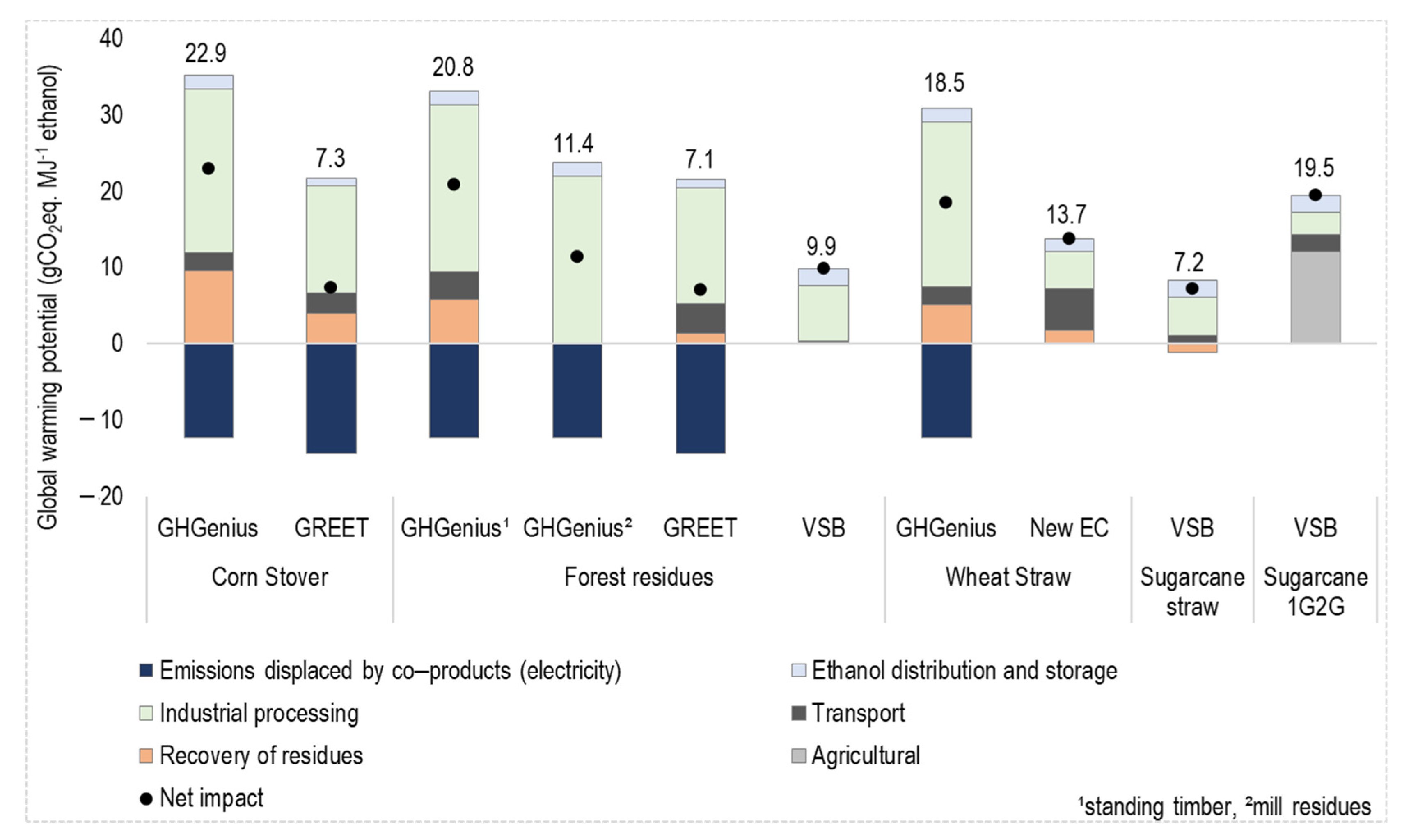
4.2. Comparison of Greenhouse Gases Emissions Calculated with the Different LCA Models

Figure 1 presents the breakdown of GHG emissions linked to 2G ethanol production pathways considering different biomass options in the four considered LCA models (data are also provided in Supplementary Material Table S1).

The net climate impact for 2G ethanol production in each LCA model varied significantly. In general, these differences can be justified by different input values and emissions factors. The key emission factors retrieved from the default 2G ethanol pathways of the four assessed models are presented in the Supplementary Material (Table S2). It is also worth mentioning that in GHGenius the emissions factors for most chemical inputs varied with the country region due to different electricity emission factors, as do nitrogen emission factors, depending on the mix of nitrogen fertilizer used.

Corn stover ethanol in GHGenius presented the highest GHG emissions among all the 2G biofuel pathways and models assessed: 22.9 gCO₂eq. MJ⁻¹. On the other hand, forest residue ethanol in GREET presented the lowest GHG emissions (7.1 gCO₂eq. MJ⁻¹). The higher diesel inputs in GHGenius justify the higher emissions in the industrial conversion phase. The New EC model and VSB did not consider energy inputs for the industrial conversion, whereas GREET and GHGenius accounted for diesel inputs in the industrial conversion of biomass into 2G ethanol. The highest emissions in the transportation phase were obtained with the New EC model. This can be justified by the comparatively higher transportation distance considered in this model (i.e., 500 km). Ethanol distribution emissions were higher in VSB compared to the other models because it considered that ethanol is only transported by heavy trucks.

In GHGenius, 2G ethanol impacts from corn stover were higher than in GREET: 22.9 gCO₂eq. MJ⁻¹ and 7.3 gCO₂eq. MJ⁻¹, respectively. The GHGenius model considered no credit or debit for carbon changes in soil, nor did it avoid emissions due to corn stover removal, whereas GREET considered avoided N₂O emissions in the field due to biomass removal (Table S3 from Supplementary Material). In GHGenius, several chemical inputs had relatively high emission factors; for example, phosphate nutrients emitted 1619 gCO₂eq. kg⁻¹ and sulfuric acid emitted 217 gCO₂eq. kg⁻¹ (Table S2), which contributed to high emissions in the industrial conversion process. There was no enzyme input in this model, since cellulase is produced on-site. In GREET, avoided LUC emissions were considered for 2G ethanol production when replacing 1G ethanol (Table S4). Although the two models accounted for emissions displaced due to electricity exported to the grid, in GREET this displacement was higher than in GHGenius, since the credit considered varied according to the electricity mix of each country. GHGenius presented higher energy inputs than GREET in the industrial conversion processes, as well as higher input of chemicals. Produced ethanol was consumed locally in both GHGenius and GREET. In addition to train and truck transportation, GREET considered barge modal for ethanol distribution (Table S5). GREET considered only local 2G ethanol consumption; consequently, there was no ocean transportation for ethanol distribution. Biomass boiler emissions and electricity output in the production of 2G from corn stover retrieved from GHGenius and GREET are presented in the Supplementary Material (Table S6).

In the case of 2G ethanol from forest residues, the three considered LCA models presented relatively similar results. Naturally, the GHGenius pathway for 2G production from standing timber presented higher GHG emissions (20.8 gCO₂eq. MJ⁻¹) than pathways using forest residues. The GHGenius model has three different options for woody biomass residues: sawmill residues, short rotation crops, and standing timber. Sawmill residues are the default feedstock in the pathway considering the version as downloaded from its website. The model does not include any procurement or transportation operations for this specific biomass feedstock. Forest residues from the standing timber pathway were selected in the analysis for a better comparison with the other models, since it includes procurement and transportation inputs of biomass feedstock. GREET considered comparably higher fuel consumption since it included mechanical operations such as stumpage and harvesting of forest residues (Table S7). In addition, all the energy consumption in forest operations, which includes harvesting, collection, extraction of residues, milling, and chipping, were allocated between timber and forest residues. VSB considered comparative low energy inputs for residue recovery, since shipping was the main operation considered. Energy inputs in GREET were higher than in the other two models. This was mostly due to the use of natural gas primarily for drying and preparing the feedstock for the conversion processes (Table S8). VSB was the only model to consider infrastructure materials (e.g., steel and concrete) in the industrial process. VSB did not include external energy inputs in the process and presented relatively lower sugar inputs and sulfuric acid compared to the other models. Similar to 2G ethanol production from corn stover, both the GHGenius and GREET models included GHG emissions displaced due to electricity exports to the grid, which varied according to the electricity mix in each country. In VSB, the GHG emission climate impacts were shared among products considering an economic allocation method. There was no ocean transportation in any of the three models, as 2G ethanol was considered only for local consumption (Table S9). Again, barge modal was considered in the GREET model. Biomass boiler emissions and electricity output are presented in the Supplementary Material (Table S10).

For 2G ethanol from wheat straw, GHGenius presented higher GHG emissions than New EC (18.5 and 13.7 gCO₂eq. MJ⁻¹, respectively). This was mostly due to the consideration of fertilizer replacement in view of straw removal (Table S11) and higher energy inputs in the industrial conversion phase in GHGenius (Table S12). In addition, GHGenius considered a list of chemical inputs that had relatively high emission factors (Table S1), and the use of diesel for operations with wheeled loaders. In GHGenius, the emission factor for diesel was 111 gCO₂eq. MJ⁻¹, whereas New EC considered 95 gCO₂eq. MJ⁻¹. Electricity output in New EC was considerably higher and this model (Table S14) considered no additional energy input for the industrial conversion stage. GHGenius considered distribution distances between potential feedstock locations and consumer markets in Canada (Table S13). Besides inland road transport modals, the New EC model included ocean transportation for ethanol distribution. Biomass boiler emissions are presented in Table S14.

VSB results for 2G ethanol from sugarcane straw (7.2 gCO₂eq. MJ⁻¹) were similar to the values obtained for 2G ethanol from corn stover and forest residues with GREET: 7.3 and 7.1 gCO₂eq. MJ⁻¹, respectively. These results are based on 2G ethanol production from agricultural residues, and thus, without GHG emissions linked to biomass production. Therefore, even small differences among the models highly influenced the results. Comparing the integrated 1G2G ethanol production with the standalone 2G ethanol conversion process from sugarcane, the emissions in the 1G2G (19.5 gCO₂eq. MJ⁻¹) were higher than in the standalone 2G process (7.2 gCO₂eq. MJ⁻¹) because the 1G2G carried part of the impacts from the sugarcane production system, whereas the standalone 2G process only used sugarcane straw as biomass feedstock (Table S15). It is worth mentioning that ethanol produced in a 1G2G process presents lower impacts than 1G ethanol from sugarcane because more ethanol is produced in the 1G2G process using the same sugarcane biomass. For instance, the carbon intensity of 1G sugarcane ethanol in Brazil was around 21 gCO₂eq. MJ⁻¹ of ethanol produced [42]. The key parameters for standalone 2G ethanol from sugarcane straw are presented in Tables S15–S18 of the Supplementary Material, and the corresponding parameters for integrated 1G2G ethanol production from sugarcane are presented in Tables S19–S22 of the Supplementary Material.

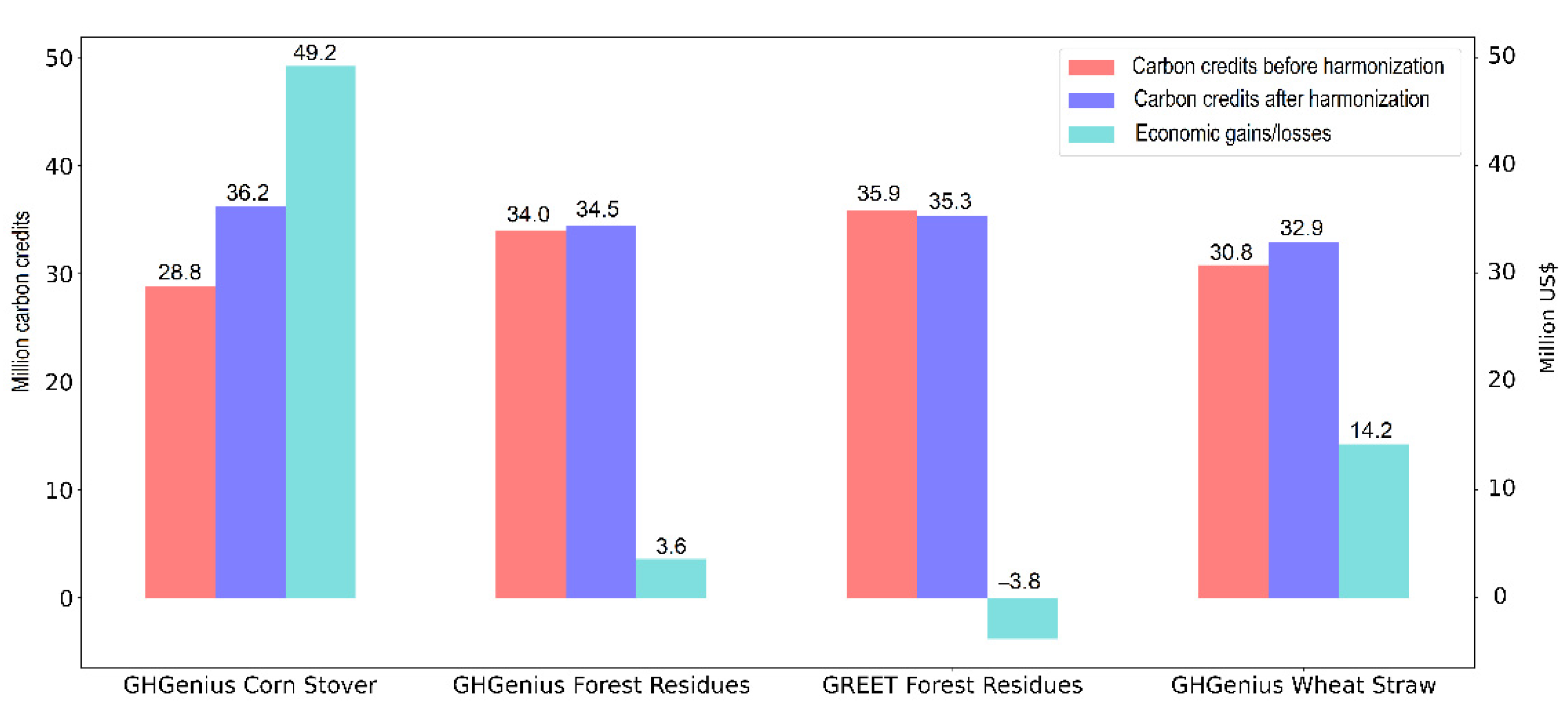
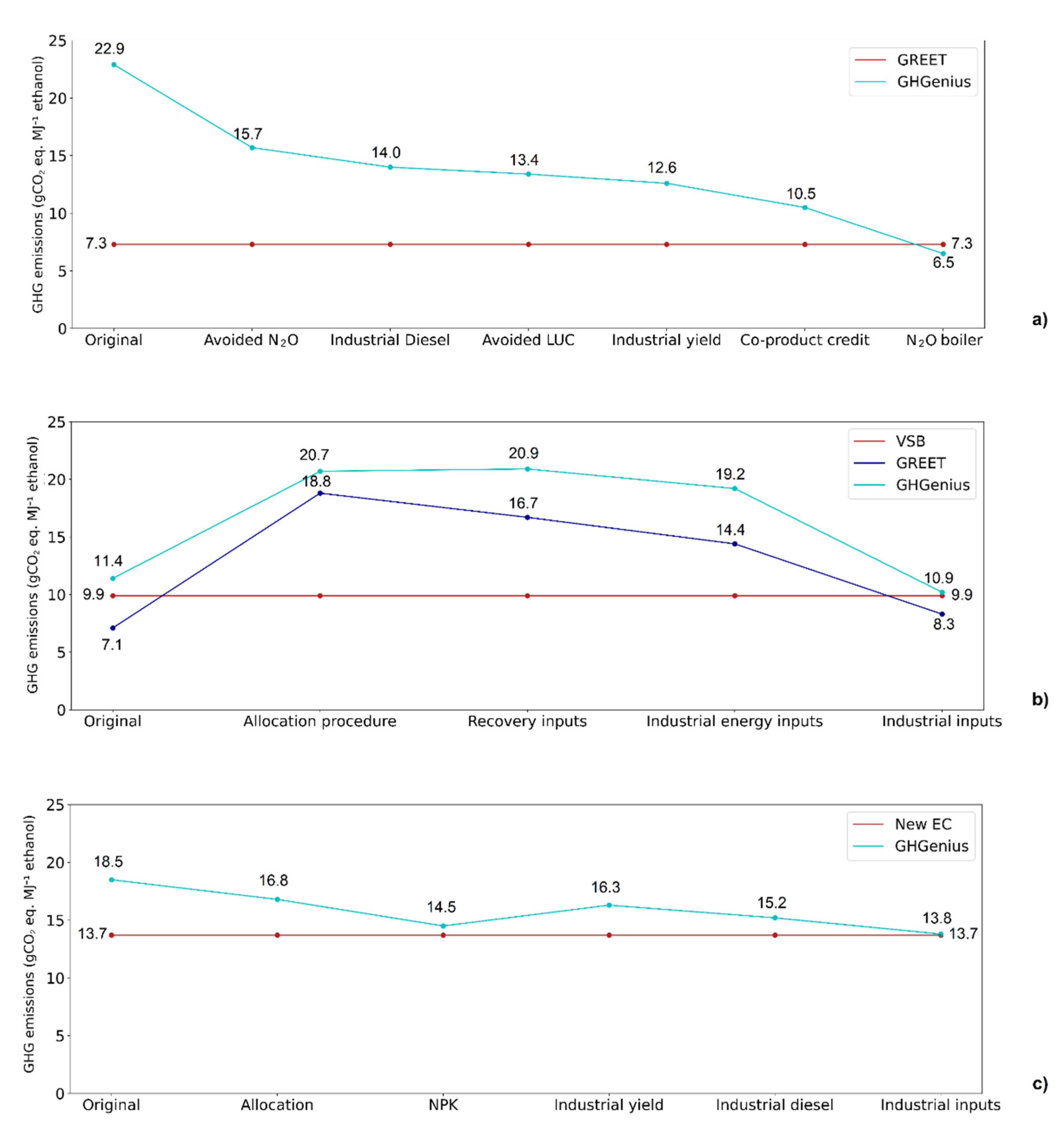
4.3. Harmonization of Greenhouse Gases Emissions of 2G Ethanol Pathways

The results obtained after the harmonization of 2G ethanol production from corn stover, forest residues, and wheat straw are presented in Figure 2. The figure presents the results on a step-by-step basis to track the impacts of harmonizing each parameter on the final carbon intensity to reach converging results.

Figure 2 indicates that the differences among the assessed models decreased considerably after harmonization of a few key parameters and methodological assumptions, reaching fairly similar results. However, some small differences among the models could still be found after the harmonization steps, as they were basically related to other particularities of each method that were not harmonized in this study. These particularities, such as different climate change characterization factors and different emission factors, may cumulatively have contributed to the difference in the global GHG emissions of the biofuel pathways.

In the case of 2G ethanol from corn stover, the harmonization of the avoided N₂O emissions presented the highest contribution to the approximate GREET and GHGenius results. The differences between the results in these two models decreased by 95%, from 15.6 gCO₂eq. MJ⁻¹ before harmonization to 0.8 gCO₂eq. MJ⁻¹ after harmonization. The sum of all harmonization steps resulted in a 72% reduction of 2G ethanol impacts in GHGenius, decreasing from 22.9 gCO₂eq. MJ⁻¹ to 6.5 gCO₂eq. MJ⁻¹. In the case of 2G ethanol from forest residues, the three models already presented fairly similar results before harmonization, even with variations among the considered data for each model, as well as different parameters and methodological assumptions. After harmonization, the models reached even more similar results. The range between GHGenius and VSB emissions decreased by 78%, from 1.5 gCO₂eq. MJ⁻¹ to 0.3 gCO₂eq. MJ⁻¹. For GREET, the range decreased by 45%, from 2.8 gCO₂eq. MJ⁻¹ to 1.5 gCO₂eq. MJ⁻¹. The largest range of different results among the models happened after harmonization of the allocation procedure; for instance, it increased GHGenius emissions by 81%, and by 166% in GREET compared to the original results. On the other hand, when the industrial conversion inputs were harmonized, it led to the largest approximation of the results; it reduced the emissions in GHGenius by 47%, and in GREET by 42%, reaching 10.2 gCO₂eq. MJ⁻¹ and 8.3 gCO₂eq. MJ⁻¹, respectively. The harmonization of 2G ethanol from wheat straw reached the most similar results among the different analyzed 2G production pathways; the initial difference of 4.8 gCO₂eq. MJ⁻¹ decreased to 0.1 gCO₂eq. MJ⁻¹. The harmonization of fertilizer inputs led to the largest approximation of results, decreasing GHGenius emissions from 16.8 gCO₂eq. MJ⁻¹ to 14.5 gCO₂eq. MJ⁻¹, a drop of 14% in its climate impacts. The step of harmonizing the industrial conversion yields increased the difference among the models from 0.8 gCO₂eq. MJ⁻¹ to 2.6 gCO₂eq. MJ⁻¹.

4.4. Implications and Opportunities for Harmonization of LCA Models

Decarbonization programs are being proposed worldwide to mitigate GHG emissions from the transportation sector [39] by establishing a credit market that financially rewards GHG reduction from low carbon fuels. To be eligible for such decarbonization programs, all fuel pathways need to demonstrate their (lower) carbon intensities to generate carbon credits, which correspond to emissions savings of renewable fuels when compared to their fossil counterparts. However, the carbon credits generated by each decarbonization program vary according to their specificities and to the methodological approach and assumptions of the LCA models from which the calculators are derived. This means that currently there is no standard calculation to generate these carbon credits worldwide. In this study, the analysis of various 2G ethanol pathways from four different biomasses identified key differences in the input data and methodological choices of each considered model. Some of them, such as divergences between allocation procedures, energy inputs, and considered avoided emissions, could be harmonized to yield fairly similar results. What was proposed and achieved in this study is that with relatively simple harmonization of LCA models and calculation tools from decarbonization programs it would be possible to reach a global system of carbon credit generation. This harmonized global carbon credit means that, independently from the regions of study and LCA model applied, the results could be fairly comparable in view of similar calculation procedures and input data. Other studies performed for biofuel pathways support the possibility of reaching similar carbon intensity results after harmonization of the models. For instance, Pereira et al. [25] assessed four LCA models considering conventional first generation (1G) ethanol production from sugarcane, corn, and wheat. After harmonization, maximum variation of GHG emissions was up to 8% for sugarcane ethanol and 3% for corn ethanol. Obnamia et al. [48] focused on the comparison of GREET and GHGenius models for assessing corn ethanol and, after harmonization, the GHG emissions variation was only 1.3 gCO₂eq. MJ⁻¹. In Bonomi et al. [53] the authors compared LCA models for fatty acid methyl ester (FAME) and hydrotreated vegetable oil/hydroprocessed ester and fatty acid (HVO/HEFA) production from soybean oil, palm oil, and used cooking oil (UCO). The maximum variation in GHG emissions from soybean FAME was 5.6 gCO₂eq. MJ⁻¹ after harmonization.

These initiatives can be a first step in creating a global carbon credit, as it was shown that it is possible to deliver similar carbon intensity results for the same fuel pathways after the harmonization of a few steps. For a better visualization of the harmonization impacts, we performed an exercise to account for the eventual economic losses and/or gains in terms of carbon credit generation after harmonization, presented in Figure 3. As a result, the harmonization of the corn stover residue 2G ethanol pathway using GREET parameters (Figure 2a) to produce 20 billion liters of ethanol would generate an additional 7.3 million carbon credits, which means that if no harmonization were done, the same 20 billion liters calculated in GHGenius would lose an additional revenue of USD 49 million. The harmonization of wheat straw considering New EC as the default (Figure 2c) would generate an additional 2 million carbon credits, equivalent to USD 14 million. In the case of forest residues (Figure 2b), harmonization using VSB as the default would lead to a gain of USD 3.6 million in the case of GHGenius, due to the generation of 0.5 million carbon credits, and to a loss of USD 3.8 million in the case of GREET, due to the reduction of 0.6 million carbon credits. These values consider USD 7 per carbon credit generated (i.e., one metric ton of avoided CO₂eq), as considered by the Brazilian RenovaBio program in 2020 [54], which is close to the USD 10 per metric ton of CO₂ considered in a similar carbon capture program (45Q tax credit) [55] (exchange rate USD 1.00 = BRL 5.16). This exercise shows that currently the carbon credits cannot be fairly compared.

5. Conclusions

We provided a detailed quantitative comparison of LCA models that are used or were adapted for the calculation tools of key decarbonization programs already in place worldwide. Such LCA models derive different carbon intensities for similar biofuel pathways. The main reasons are differences in considered emission factors for chemicals, energy, and other inputs; the models differ in assumptions for biomass production and residue recovery, allocation procedures, conversion yields, and energy inputs, among others. The harmonization proposed in this study for 2G ethanol production pathways showed that it is possible to align the outcomes of LCA models through a series of harmonization steps, selecting only a few key parameters and methodological assumptions, which means that with relatively small efforts, LCA models and decarbonization programs could improve their transparency and derive comparable results. After harmonization, differences among 2G ethanol from wheat straw were limited to 0.1 gCO₂eq. MJ⁻¹, and discrepancies in emissions decreased by 95% and 78% for corn stover and forest residues, respectively.

We concluded that there is still room to standardize the models and an effort to update the databases and to harmonize the inputs for the more important biofuels technological pathways would make them more consistent. It would be fundamental to better estimate GHG emissions of biofuels systems, which could be a first step towards a globally accepted and exchangeable carbon credit system. This would benefit decarbonization programs, researchers, and policymakers alike, as the comparisons between emissions and corresponding climate impacts among different biofuels would be easily comparable and communicable.

References

1. Daioglou, V.; Doelman, J.; Wicke, B.; Faaij, A.; van Vuuren, D. Integrated assessment of biomass supply and demand in climate change mitigation scenarios. Glob. Environ. Chang. 2019, 54, 88–101. [Google Scholar] [CrossRef] [Green Version]
2. Hanssen, S.V.; Daioglou, V.; Steinmann, J.N.Z.; Frank, S.; Popp, A.; Brunelle, T.; Lauri, P.; Hasewaga, T.; Huijbregts, M.A.J.; van Vuuren, D.P. Biomass residues as twenty-first century bioenergy feedstock—A comparison of eight integrated assessment models. Clim. Chang. 2019, 163, 1569–1586. [Google Scholar] [CrossRef] [Green Version]
3. OECD/IEA. Technology Roadmap Delivering Sustainable Bioenergy. 2017. Available online: https://www.ieabioenergy.com/publications/technology-roadmap-delivering-sustainable-bioenergy/ (accessed on 20 July 2020).
4. Slade, R.; Bauen, A.; Gross, R. Global bioenergy resources. Nat. Clim. Chang. 2014, 4, 99–105. [Google Scholar] [CrossRef]
5. Adebayo, T.S.; Awosusi, A.A.; Oladipupo, S.D.; Agyekum, E.B.; Jayakumar, A.; Kumar, N.M. Dominance of fossil fuels in Japan′s national energy mix and implications for environmental sustainability. Int. J. Environ. Res. Public Health 2021, 18, 7347. [Google Scholar] [CrossRef]
6. Baeyens, J.; Kang, Q.; Appels, L.; Dewil, R.; Lv, Y.; Tan, T. Challenges and opportunities in improving the production of bio-ethanol. Prog. Energy Combust. Sci. 2015, 47, 60–88. [Google Scholar] [CrossRef]
7. Lynd, L.R.; Liang, X.; Biddy, M.J.; Allee, A.; Cai, H.; Foust, T.; Himmel, M.E.; Laser, M.S.; Wang, M.; Wyman, C.E. Cellulosic ethanol: Status and innovation. Curr. Option Biotechnol. 2017, 45, 202–211. [Google Scholar] [CrossRef] [Green Version]
8. Wang, M.; Han, J.; Dunn, J.B.; Cai, H.; Elgowainy, A. Well-to-wheels energy use and greenhouse gas emissions of ethanol from corn, sugarcane and cellulosic biomass for US use. Environ. Res. Lett. 2012, 7, 045905. [Google Scholar] [CrossRef] [Green Version]
9. Zabed, H.; Sahu, J.N.; Suely, A.; Boyce, A.N.; Faruq, G. Bioethanol production from renewable sources: Current perspectives and technological progress. Renew. Sustain. Energy Rev. 2017, 71, 475–501. [Google Scholar] [CrossRef]
10. Zhao, Y.; Damgaard, A.; Christensen, T.H. Bioethanol from corn stover: A review and technical assessment of alternative biotechnologies. Prog. Energy Combust. Sci. 2018, 67, 275–291. [Google Scholar] [CrossRef] [Green Version]
11. Jaiswal, D.; de Souza, A.; Larsen, S.; LeBauer, D.S.; Miguez, F.; Sparovek, G.; Bollero, G.; Buckeridge, M.S.; Long, S.P. Brazilian sugarcane ethanol as an expandable green alternative to crude oil use. Nat. Clim. Chang. 2017, 7, 788–791. [Google Scholar] [CrossRef]
12. Prasad, S.; Singh, A.; Korres, N.E.; Rathore, D.; Sevda, S.; Pant, D. Sustainable utilization of crop residues for energy generation: A life cycle assessment (LCA) perspective. Bioresour. Technol. 2020, 303, 122964. [Google Scholar] [CrossRef]
13. World Bioenergy Association. WBA Global Bioenergy Statistics. 2016. Available online: https://worldbioenergy.org/uploads/WBA%20Global%20Bioenergy%20Statistics%202016.pdf (accessed on 20 July 2020).
14. SCOPE. Bioenergy & Sustainability: Bridging the Gaps; Souza, G.M., Victoria, R.L., Joly, C.A., Verdade, L.M., Eds.; SCOPE: Paris, France, 2012; ISBN 978-2-9545557-0-6. [Google Scholar]
15. CGEE. Sustainability of Sugarcane Bioenergy. Brasília, DF, Brasil. 2012. Available online: http://livroaberto.ibict.br/bitstream/1/910/1/Sustainability_sugarcane_bioenergy.pdf (accessed on 20 July 2020).
16. Manochio, C.; Andrade, B.R.; Rodriguez, R.P.; Moraes, B.S. Ethanol from biomass: A comparative overview. Renew. Sustain. Energy Rev. 2017, 80, 743–755. [Google Scholar] [CrossRef]
17. Cavalett, O.; Chagas, M.F.; Junqueira, T.L.; Watanabe, M.D.B.; Bonomi, A. Environmental impacts of technology learning curve for cellulosic ethanol in Brazil. Ind. Crop. Prod. 2017, 106, 31–39. [Google Scholar] [CrossRef]
18. Junqueira, T.L.; Chagas, M.F.; Gouveia, V.L.; Rezende, M.; Watanabe, M.D.B.; Jesus, C.; Cavalett, O.; Milanez, A.; Bonomi, A. Techno-economic analysis and climate change impacts of sugarcane biorefineries considering different time horizons. Biotechnol. Biofuels 2017, 10, 50. [Google Scholar] [CrossRef] [Green Version]
19. California Air Resource Board. Low Carbon Fuel Standard. 2020. Available online: https://ww2.arb.ca.gov/our-work/programs/low-carbon-fuel-standard (accessed on 14 July 2021).
20. British Columbia. Greenhouse Gas Reduction (Renewable and Low Carbon Fuel Requirements) Act Renewable and Low Carbon Fuel Requirements Regulation B.C. Reg. 394/2008. Consolidation current to August 7, 2020. Available online: https://www.bclaws.ca/civix/document/id/crbc/crbc/394_2008 (accessed on 13 November 2020).
21. EU. Directive (EU) 2018/2001 of the European Parliament and of the Council of 11 December 2018. 2018. Available online: https://eur-lex.europa.eu/legal-content/EN/TXT/?uri=uriserv:OJ.L_.2018.328.01.0082.01.ENG&toc=OJ:L:2018:328:TOC (accessed on 13 November 2020).
22. ANP. Agência Nacional do Petróleo, Gás Natural e Biocombustíveis. RenovaBio. 2020. Available online: http://www.anp.gov.br/producao-de-biocombustiveis/renovabio (accessed on 13 November 2020).
23. Peña, C.; Civit, B.; Gallego-Schmid, A.; Druckman, A.; Caldeira-Pires, A.; Weidema, B.; Mieras, E.; Wang, F.; Fava, J.; Canals, L.M.; et al. Using life cycle assessment to achieve a circular economy. Int. J. Life Cycle Assess. 2021, 26, 215–220. [Google Scholar] [CrossRef]
24. Gerbrandt, K.; Chu, P.L.; Simmonds, A.; Mullins, K.A.; MacLean, H.L.; Griffin, M.W.; Saville, B.A. Life cycle assessment of lignocellulosic ethanol: A review of key factors and methods affecting calculated GHG emissions and energy use. Curr. Opin. Biotechnol. 2016, 38, 63–70. [Google Scholar] [CrossRef]
25. Pereira, L.G.; Cavalett, O.; Bonomi, A.; Zhang, Y.; Warner, E.; Chum, H.L. Comparison of biofuel life-cycle GHG emissions assessment tools: The case studies of ethanol produced from sugarcane, corn, and wheat. Renew. Sustain. Energy Rev. 2019, 110, 1–12. [Google Scholar] [CrossRef]
26. Bonomi, A.; Cavalett, O.; Cunha, M.P.; Lima, M.A.P. Virtual Biorefinery—An Optimization Strategy for Renewable Carbon Valorization; Springer International Publishing: Kamm, Switzerland, 2016. [Google Scholar]
27. Cherubini, F.; Strømman, A.H.; Ulgiati, S. Influence of allocation methods on the environmental performance of biorefinery products—A case study. Resour. Conserv. Recycl. 2011, 55, 1070–1077. [Google Scholar] [CrossRef]
28. Cherubini, F.; Fuglestvedt, J.; Gasser, T.; Reisinger, A.; Cavalett, O.; Huijbregts, M.A.J.; Levasseur, A. Bridging the gap between impact assessment methods and climate science. Environ. Sci. Policy 2016, 64, 129–140. [Google Scholar] [CrossRef] [Green Version]
29. Hoefnagels, R.; Smeets, E.; Faaij, A. Greenhouse gas footprints of different biofuel production systems. Renew. Sustain. Energy Rev. 2010, 14, 1661–1694. [Google Scholar] [CrossRef]
30. RFA. Renewable Fuel Associations—Statistics Annual World Fuel Ethanol Production (Mil. Gal.). 2021. Available online: https://ethanolrfa.org/statistics/annual-ethanol-production/ (accessed on 13 August 2021).
31. CARB. California Air Resource Board. LCFS Basics with Notes. 2020. Available online: https://ww2.arb.ca.gov/sites/default/files/2020-09/basics-notes.pdf (accessed on 14 July 2021).
32. CARB. California Air Resource Board. CA-GREET3.0 Supplemental Document and Tables of Changes. 2018. Available online: https://ww2.arb.ca.gov/sites/default/files/classic//fuels/lcfs/ca-greet/cagreet_supp_doc_clean.pdf (accessed on 14 July 2021).
33. OR. Oregon′s Clean Fuels Program. Fuel Pathways—Carbon Intensity Values. 2021. Available online: https://www.oregon.gov/deq/ghgp/cfp/Pages/Clean-Fuel-Pathways.aspx (accessed on 28 January 2021).
34. British Columbia. Renewable & Low Carbon Fuel Requirements Regulation. 2020. Available online: https://www2.gov.bc.ca/gov/content/industry/electricity-alternative-energy/transportation-energies/renewable-low-carbon-fuels (accessed on 13 November 2020).
35. British Columbia. Using GHGenius in B.C. 2017. Available online: https://www2.gov.bc.ca/assets/gov/farming-natural-resources-and-industry/electricity-alternative-energy/transportation/renewable-low-carbon-fuels/rlcf010_-_using_ghgenius_for_bc.pdf (accessed on 13 November 2020).
36. California. Clean Fuel Standard. 2020. Available online: https://www.canada.ca/en/environment-climate-change/services/managing-pollution/energy-production/fuel-regulations/clean-fuel-standard.html (accessed on 14 July 2021).
37. California. Clean Fuel Standard: Proposed Regulatory Approach. 2020. Available online: https://www.canada.ca/en/environment-climate-change/services/managing-pollution/energy-production/fuel-regulations/clean-fuel-standard/regulatory-approach.html#toc55 (accessed on 14 July 2021).
38. EU. Directive 2009/28/EC of the European Parliament and of the Council of 23 April 2009. 2009. Available online: https://eur-lex.europa.eu/legal-content/EN/TXT/PDF/?uri=CELEX:32009L0028&from=EN (accessed on 13 November 2020).
39. Edwards, R.; O′Connell, A.; Padella, M.; Giuntoli, J.; Koeble, R.; Bulgheroni, C.; Marelli, L.; Lonza, L. Definition of Input Data to Assess GHG Default Emissions from Biofuels in EU Legislation. Version 1d. 2019. Available online: https://ec.europa.eu/jrc/en/publication/definition-input-data-assess-ghg-default-emissions-biofuels-eu-legislation (accessed on 13 November 2020).
40. CNPEM. Relatório Anual 2019 Partes II e III. 2019. Available online: https://cnpem.br/wp-content/uploads/2019/09/RelatorioCG-2019-Parte-IIeIII.pdf (accessed on 13 November 2020).
41. Klein, B.C.; Chagas, M.F.; Watanabe, M.D.B.; Bonomi, A.; Maciel Filho, R. Low carbon biofuels and the New Brazilian National Biofuel Policy (RenovaBio): A case study for sugarcane mills and integrated sugarcane-microalgae biorefineries. Renew. Sustain. Energy Rev. 2018, 115, 109365. [Google Scholar] [CrossRef]
42. Matsuura, M.I.S.F.; Scachetti, M.T.; Chagas, M.F.; Seabra, J.; Moreira, M.M.R.; Bonomi, A.; Bayma, G.; Picoli, J.F.; Morandi, M.A.B.; Ramos, N.P.; et al. RenovaCalcMD: Método e Ferramenta Para a Contabilidade da Intensidade de Carbono de Biocombustíveis no Programa RenovaBio. 2018. Available online: http://www.anp.gov.br/images/Consultas_publicas/2018/n10/CP10-2018_Nota-Tecnica-Renova-Calc.pdf (accessed on 20 July 2020).
43. (S&T)2 Consultants Inc. GHGenius Model 5.0c. 2018. Available online: https://ghgenius.ca/index.php/downloads (accessed on 20 July 2020).
44. ANL. GREET Model. 2018. Available online: https://greet.es.anl.gov/ (accessed on 20 July 2020).
45. Edwards, R.; Padella, M.; Giuntoli, J.; Koeble, R.; O’Connell, A.; Bulgheroni, C.; Marelli, L. Biofuels Pathways. Input Values and GHG Emissions. Database (COM(2016)767). European Commission, Joint Research Centre (JRC) [Dataset]. 2016. Available online: http://data.europa.eu/89h/jrc-alf-bio-biofuels_jrc_annexv_com2016-767_v1_july17 (accessed on 20 July 2020).
46. Bonomi, A.; Cavalett, O.; Klein, B.C.; Chagas, M.F.; Souza, N.R.D. Technical Report—Comparison of Biofuel Life Cycle Analysis Tools, Phase 2, Part 2: Comparison of LCA Models for Biochemical Second Generation (2G) Ethanol Production and Distribution. IEA Bioenergy. Task 39—Commercializing Liquid Biofuels. 2020. Available online: http://task39.sites.olt.ubc.ca/files/2020/01/Task-39-Phase-2.2-Ethanol-2G-Comparison-of-Biofuel-Life-Cycle-Analysis-Tools.pdf (accessed on 10 July 2021).
47. IPCC. Climate Change 2007—The Physical Science Basis. Contribution of Working Group I to the Fourth Assessment Report of the IPCC; Cambridge University Press: Cambridge, UK, 2007; ISBN 978 0521 88009-1. [Google Scholar]
48. Obnamia, J.A.; Dias, G.M.; MacLean, H.L.; Saville, B.A. Comparison of U.S. Midwest corn stover ethanol greenhouse gas emissions from GREET and GHGenius. Appl. Energy 2019, 235, 591–601. [Google Scholar] [CrossRef]
49. Edwards, R.; Padella, M.; Giuntoli, J.; Koeble, R.; O’Connell, A.; Bulgheroni, C.; Marelli, L. Appendix 1—Outcomes of Stakeholders Consultations. Definition of Input Data to Assess GHG Default Emissions from Biofuels in EU Legislation, Version 1c—July 2017, EUR 28349 EN; Publications Office of the European Union: Luxembourg, 2017; ISBN 978-92-79-66185-3. [Google Scholar] [CrossRef]
50. Humbird, D.; Davis, R.; Tao, L.; Kinchin, C.; Hsu, D.; Aden, A.; Schoen, P.; Lukas, J.; Olthof, B.; Worley, M.; et al. Process Design and Economics for Biochemical Conversion of Lignocellulosic Biomass to Ethanol. NREL. 2011. Available online: https://www.nrel.gov/docs/fy11osti/47764.pdf (accessed on 20 July 2020).
51. Wu, M.; Wang, M.; Huo, H. Fuel-Cycle Assessment of Selected Bioethanol Production Pathways in the United States. 2006. Available online: https://greet.es.anl.gov/files/2lli584z (accessed on 20 July 2020.).
52. Johnson, E. Integrated enzyme production lowers the cost of cellulosic ethanol. Biofuels Bioprod. Biorefining 2016. [Google Scholar] [CrossRef] [Green Version]
53. Bonomi, A.; Klein, B.C.; Chagas, M.F.; Souza, N.R.D. Technical Report—Comparison of Biofuel Life Cycle Analysis Tools. Phase 2, Part 1: FAME and HVO/HEFA. IEA Bioenergy. Task 39—Commercializing Liquid Biofuels. 2019. Available online: http://task39.sites.olt.ubc.ca/files/2019/08/Task-39-CTBE-biofuels-LCA-comparison-Final-Report-Phase-2-Part-1-2019.pdf (accessed on 10 July 2021).
54. B3. Renda Fixa. Dados Por Ativo. 2021. Available online: http://www.b3.com.br/pt_br/market-data-e-indices/servicos-de-dados/market-data/historico/renda-fixa/ (accessed on 21 January 2021).
55. 26 U.S. Code § 45Q—Credit for Carbon Oxide Sequestration. Available online: https://www.law.cornell.edu/uscode/text/26/45Q (accessed on 20 August 2021).
Figure 1. Breakdown of GHG emissions of 2G ethanol production pathways for the four biomass and four LCA models considered.
Sustainability 13 10371 g001
Figure 2. Harmonization of key parameters and assumptions regarding the GHG emissions of 2G ethanol from corn stover considering the inclusion of GREET values in GHGenius (panel (a)), forest residues with the inclusion of VSB values in GHGenius and GREET (panel (b)), and wheat straw considering the inclusion of New EC values in GHGenius (panel (c)).
Sustainability 13 10371 g002
Figure 3. Economic gains and/or losses from the difference in carbon credit generation after the harmonization of LCA models.
Sustainability 13 10371 g003