Restructuring State Intervention Strategies towards Chickpea Production Development in India—Application of Structural Equation Modeling (SEM)

Abstract

Structural equation modeling (SEM) was employed to analyze the influence of exogenous variables (research and extension (RE), marketing aspects (MA), and infrastructure development (ID)) on the endogenous variable chickpea production development (CPD) to restructure policy interventions in India. Results of the measurement model revealed that all the latent variables have construct validity (both convergent validity and discriminant validity) and composite reliability. Confirmatory factor analysis revealed that all indicators of both exogenous and endogenous variables are significant. Yield-increasing production technologies (PT), minimum support prices (MSP), and storage structures (SS) and the three exogenous variables (research and extension, marketing, and infrastructure development) are the strongest indicators. For the endogenous variable CPD, remunerative prices (RP) is the strongest indicator and also serves as a driving force for other indicators. The results of the structural model revealed that RE is the most effective construct followed by ID and MA, and they cumulatively explained 89 percent of the total variation in CPD. Among these three constructs, MSP is the key indicator of MA with the highest loading factor (0.799), and hence it should be given the highest priority for promoting CPD in India.

1. Introduction

Legumes, also known as pulses, constitute an integral component of a sustainable crop production system as they contribute high-quality protein, free atmospheric nitrogen, can be cultivated under irrigated/dry conditions with low water requirements, are highly remunerative to farmers, and have persistent increasing demand from consumers. In 2018, the world production of pulses was around 92 m. tonnes, and the production increased drastically by about 63 per cent during 1998–2018 compared with only a 12 per cent increase from 1978 to 1998 [1]. Substantial increases have been observed in the production of common beans (+14 m. tonnes), chickpeas (+8.3 m. tonnes), lentils and pigeon peas (+3.6 m. tonnes each), cowpeas (+3.5 m. tonnes), and dry peas (+1.2 m. tonnes) at a global level. In terms of regions, production increased by 17.3 m. tonnes in Asia (with South Asia contributing a 69% share), 10.5 m. tonnes in sub-Saharan Africa, 4.8 m. tonnes in North America, and 2.2 m. tonnes in Latin America and the Caribbean [2]. This growing popularity of pulse production during the most recent decades, 1998–2018, is due to the adoption of improved varieties, plant protection aspects, advances in farm mechanization and production technologies, rise in international prices, etc. These factors coupled with increasing demand for pulses in the international market have led to favorable terms of trade across countries such as the USA, Canada, and Australia [3].

India leads in production, consumption and import of pulses during the triennium ending (TE) 2019, and it accounts for 37 per cent and 27 per cent in terms of global area and production, respectively. However, India lags in terms of productivity of pulses, with only 707 kg/ha (ranked 137th in the world) compared with a global average productivity of 1479 kg/ha during TE 2019. Ireland (4695 kg/ha) enjoyed the highest productivity in the world followed by Belgium (4211 kg/ha), the Netherlands (4049 kg/ha), Tajikistan (3683 kg/ha), and Denmark (3637 kg/ha) during TE 2019 [1]. Consequently, the pulse production in India during 2019 was 23.40 m. tonnes, which was 9.8 per cent less than the targeted 25.95 m. tonnes [4].

In India, there is a declining contribution of pulses among total food grains in terms of shares in the area, production, and productivity during the reference period, 1950–1951 to 2018–2019 (

Table 1. Contribution of pulses to the food grains basket in India (area: m. ha, production: m. tonnes, yield: kg/ha).

Year	Pulses			Food Grains			Share of Pulses in Food Grains (%)
	Area	Production	Productivity	Area	Production	Productivity	Area	Production	Productivity
1950–1951	19.09	8.41	441	97.32	50.82	522	20	17	84
1960–1961	23.56	12.7	539	115.58	82.02	710	20	15	76
1970–1971	22.54	11.82	524	124.32	108.42	872	18	11	60
1980–1981	22.46	10.63	473	126.67	129.59	1023	18	8	46
1990–1991	24.66	14.26	578	127.84	176.39	1380	19	8	42
2000–2001	20.35	11.08	544	121.05	196.81	1626	17	6	33
2010–2011	26.4	18.24	691	126.67	244.49	1930	21	7	36
2011–2012	24.46	17.09	699	124.76	259.32	2079	20	7	34
2012–2013	23.25	18.34	789	120.77	257.12	2129	19	7	37
2013–2014	25.21	19.25	764	125.04	265.04	2120	20	7	36
2014–2015	23.1	17.16	743	122.07	252.67	2069	19	7	36
2015–2016	24.91	16.35	656	123.22	251.57	2042	20	7	32
2016–2017	29.28	22.4	765	127.6	273.38	2142	23	8	36
2017–2018	29.36	24.51	835	126.98	279.51	2201	23	9	38
2018–2019	29.03	23.40	806	123.94	284.95	2299	23	8	35

Source: [4].

). This implies that there has been no breakthrough in pulse production technologies as compared to other commodities (cereals especially) of food grains. Due to low productivity, the pulse production in India has not kept pace with the growth of population, leading to their declining per capita availability (

Table 2. Per capita availability of pulses in India.

Year	Availability of Pulses
	(Grams Per Capita Per Day)	(kg Per Capita Per Year)
1951	60.7	22.1
1961	69.0	25.2
1971	51.2	18.7
1981	37.5	13.7
1991	41.6	15.2
2001	30.0	10.9
2011	43.0	15.7
2015	43.8	16.0
2016	43.0	15.7
2017	54.7	20
2018	51.3	18.7
2019	47.9	17.5

Source: [4].

). The per capita per day (gm/day) and per capita per year (kg/year) availability of pulses has dwindled between 1951 and 2019, implying that rapid growth in population has affected the availability of pulses on a per capita basis [4]. These trends have been recognized for a long time and have prompted the Government of India to introduce various programs such as the Pulses Development Scheme during IV Five Year Plan (FYP) (1969–1970 to 1973–1974), National Pulses Development Project (NPDP) during VII FYP, Special Food Grain Production Programme (SFPP) on Pulses during 1988–1989 on a 100 per cent Central Assistance basis, Integrated Scheme for Oilseeds, Pulses, Oil palm and Maize (ISOPOM) during 2004–2005 to 2009–2010, and National Food Security Mission (NFSM) during XI and XII FYPs [3].

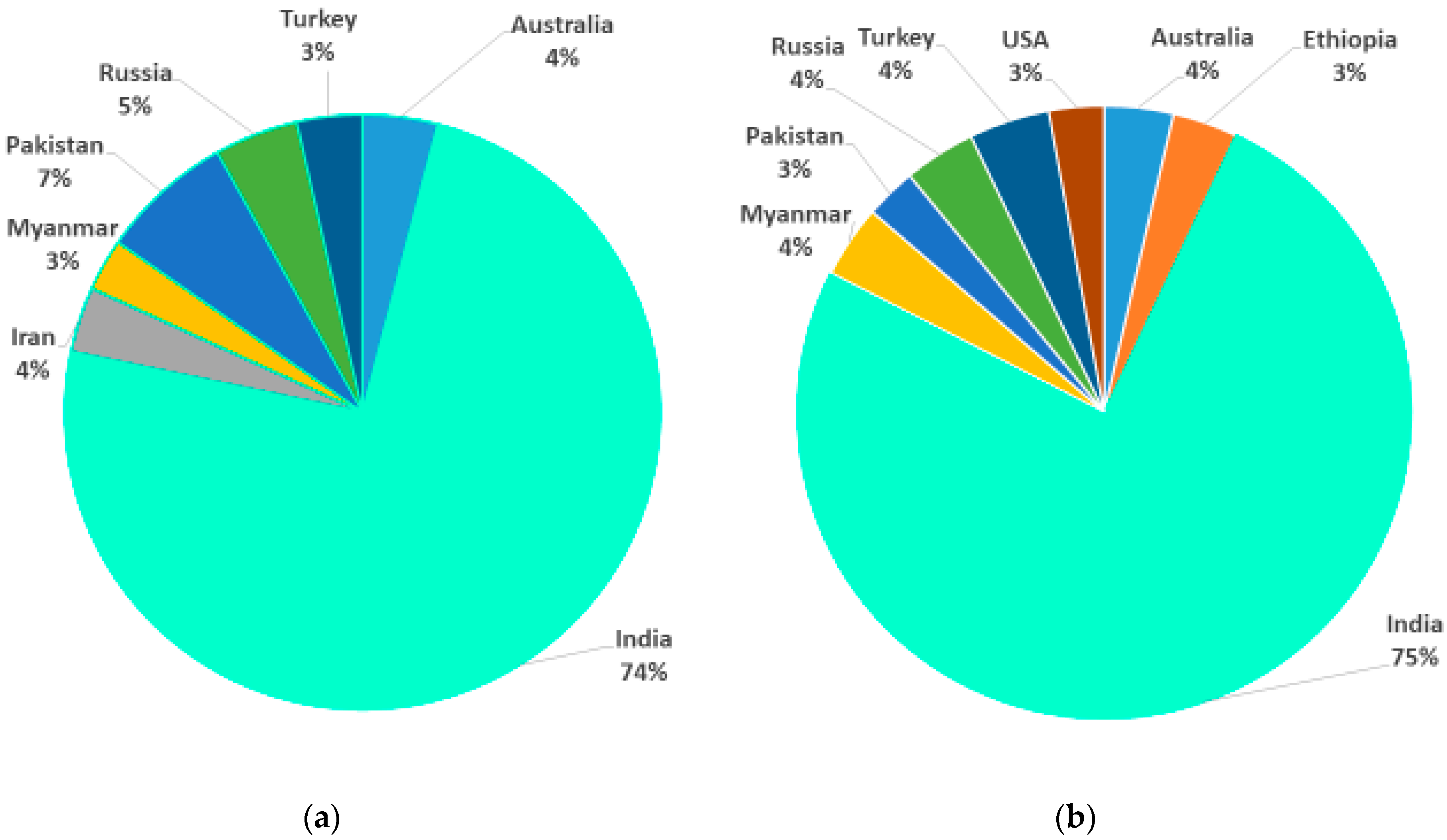
India is also the leading producer of chickpeas with an 11.23 per cent share in global pulse production [4]; chickpeas were cultivated in around 9.91 m. ha with a production of 10.23 m. tonnes during TE 2019. India contributed 74 per cent of the total area and 75 per cent of the total production of chickpeas in the world during TE 2019 (Figure 1a,b). The major chickpea-producing countries in the world were India followed by Turkey (0.58 m. tonnes), Myanmar (0.52 m. tonnes), Russia (0.51 m. tonnes), Australia (0.49 m. tonnes), Ethiopia (0.46 m. tonnes), USA (0.39 m. tonnes), and Pakistan (0.37 m. tonnes) [1]. Jordan enjoyed the highest productivity of chickpeas (5888 kg/ha) in the world, while India ranked in 29th position in the world in terms of productivity with 1031 kg/ha, which was less than the global average (1577 kg/ha), during TE 2019. Madhya Pradesh, Rajasthan, and Maharashtra are the leading chickpea-producing states in India, accounting for 43.29 per cent of total pulse production. The highest productivity of 1344 kg/ha is in Madhya Pradesh followed by 1324 kg/ha in Gujarat, 1272 kg/ha in Uttar Pradesh, and 1103 kg/ha in Rajasthan. However, the average productivity of chickpeas in India is low with 1031 kg/ha compared with the global average of 1577 kg/ha during TE 2019, as 65 per cent of the total cultivated area is under rainfed conditions and the remaining (35%) under critical irrigation support. Though the productivity of chickpeas is comparatively low, India is the leading producer in the world. However, due to stagnant productivity over the years (2001–2002 to 2016–2017), chickpea imports have been increased considerably to counterbalance its limited domestic supply. Hence, India became the leading importer of chickpeas (0.98 m. tonnes, accounting for 17.5% of total pulse imports) during 2017–18 [4]. The countries that export chickpeas to India are Canada, Australia, Iran, Myanmar, Tanzania, Pakistan, Turkey, and France. Among pulses, chickpeas contribute the single largest share in India’s export market, registering 80.02 per cent during 2019 [4]. Further, India is also a major exporter of chickpeas ranking third, i.e., 0.21 m. tonnes during 2019 [1], and its export destinations are the USA, UK, Saudi Arabia, UAE, Sri Lanka, and Malaysia.

However, the cultivation of chickpeas is not very attractive for farmers in India because of both technology and policy shortcomings. Regarding technology, there is a dearth of short-duration, high-yielding, and drought, pest, and disease-resistant varieties of chickpea. Despite the execution of the various programs mentioned earlier, their continuation to the farmers’ fields has been limited. With regard to policy, the minimum support prices (MSP) for chickpeas announced by the Government of India showed a drastic increase from Rs 1200 to Rs 4875 (306.25 per cent) during 2001 to 2019 [4]. However, this rise in MSP does not benefit the farmers because of two reasons. First, the procurement of chickpeas by government agencies is not as wide as that of cereals and especially the smallholder farmers with low marketable surplus are selling their produce in local markets for immediate cash requirements [5]. Therefore, even if the prices of chickpeas rise during the lean marketing season, this benefits the traders more than the farmers, as traders have the capacity to store. The second reason is that the availability of modern production technology, the marketing infrastructure, and the research and extension network are weak. Added to this, supply chain bottlenecks further aggravate the problems of farmers. Further, due to increasing irrigation water and electric power scarcities, changing research priorities, declining domestic and export market competitiveness of chickpeas, and increasing emphasis on supply chain mechanisms, the new millennium has posed various challenges to the development agenda for CPD in India [3]. As chickpea productivity in India (1031 kg/ha) was very low compared with Jordan (5888 kg/ha), China (5382 kg/ha), Israel (4242 kg/ha), Sudan (4048 kg/ha), Egypt (2410 kg/ha), Argentina (1961 kg/ha), and the global average (1577 kg/ha) during TE 2019, its production is not on par with the increasing demand [6]. This requires a holistic approach towards CPD in India. 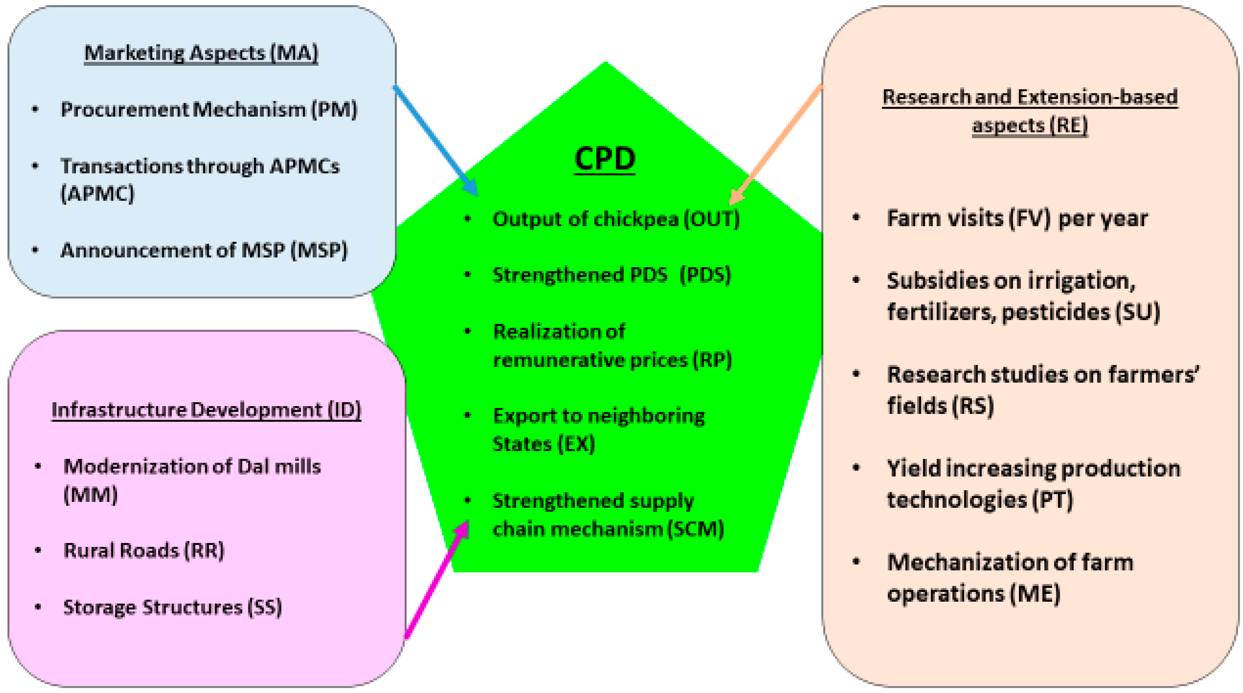The Agreement on Agriculture (AoA) of the World Trade Agreement sets out a number of general and measure-specific criteria which, when met, allow measures to be placed in the Green Box [1]. Therefore, measures such as research, extension, marketing, investments, and price support to farmers, offered by the government, can be exempted from reduction commitments and, indeed, can even be increased without any financial limitation. This is considered important because the Government of India is spending millions of rupees to ensure self-sufficiency in pulse production in general and chickpea production in particular. Besides this, the identification of various issues pertaining to research and extension (RE)-based aspects, infrastructure development (ID), and marketing aspects (MA) highlighted in Figure 2 and an understanding of their role in contributing to CPD in India have become a necessity to improve both cost effectiveness and profitability. Prioritizing the above three exogenous variables and their corresponding indicator variables is very much essential to promote CPD. However, to ensure this, we need to follow a holistic approach for analyzing and evaluating the above variables across the major chickpea-cultivating states in India. This will help to understand the intricacies of the system and to analyze in advance the effects of changes in various variables on the outcome variable (CPD). Accordingly, this in-depth study is proposed with the following specific objectives:

• To examine the association between exogenous latent variables and their corresponding indicator variables towards contributing to CPD (endogenous latent variable) in India.
• To evaluate and prioritize the contributions of both exogenous latent variables and their corresponding indicator variables in CPD using structural equation modeling (SEM).
• To suggest policy measures that contribute to CPD in India.

Accordingly, this study identified three major areas of intervention: research and extension (RE), marketing aspects (MA), and infrastructure development (ID) to ascertain and prioritize their contribution to CPD through employing SEM. The remainder of the article is structured as follows: The next section presents a brief literature review on applications of the SEM technique, followed by a section that discusses the conceptual framework and hypotheses. The methodology, sample size, and SEM technique are discussed in the fourth section. The results of the study are discussed in the fifth section. Finally, concluding remarks and suggestions for future research are presented in last section.

2. Literature Review

SEM is useful for understanding the structural linkages between a set of latent variables that contribute to the trends in actual variables. These linkages can help in identifying the policy variables that could influence the outcome variables a policy maker is interested in and in prioritizing investments. Asadi et al., 2013 [7] in their study analyzed the effects of ecological, social, and economic factors on sustainable agricultural development in Qazvin Province of Iran. Their study revealed that ecological sustainability had a greater impact on agricultural sustainability (0.642) than economic (0.604) and social (0.568) sustainability. They showed that SEM could be helpful for agricultural planners in identifying appropriate policies and monitoring the effectiveness of policy interventions.

Rohaeni et al., 2014 [8] analyzed the sustainability of cattle farming using SEM in Tanah Laut Regency, South Kalimantan, Indonesia. They selected seven exogenous variables (environmental, economic, social, technology, physical, human, and institutional resources) and two endogenous variables (cattle farming sustainability and welfare of farmers) in formulating an SEM model. The findings revealed that environmental, economic, technological, physical, human, and institutional resources influenced the sustainability of beef cattle farming; environmental, economic, technological, physical, human, and institutional resources influenced, either directly or indirectly, the welfare of farmers; and cattle farming sustainability influenced the welfare of farmers. Their study further highlighted that improvements in resources, viz., environmental, economic, technological, physical, human, and institutional resources, are sine qua non for the welfare of cattle farmers in the study area.

Muhammad et al., 2015 [9] formulated an SEM model to analyze the sustainability of paddy farming in an Integrated Agricultural Development Area (IADA), Ketara, Malaysia. The findings indicated that technological advancement is the primary positive factor that determined the level of paddy sustainability. The economy, society, and institutions were also positive factors. The study concluded that technological advancement is the most crucial element for achieving sustainability in the paddy sector.

Matin et al., 2017 [10] developed an empirical model of the supply chain management (SCM) of tomato companies in Iran. The SCM construct with six indicators (information sharing, long-term relationship, cooperation, quality, flexibility, and delivery) was employed with data collected from 20 different tomato companies. The selected indicators exerted significant positive impacts on the export of tomatoes and helped middle-line managers to know which components and practices SCM are essential to improve the export of tomatoes from Iran.

Emel et al., 2020 [11] applied SEM to analyze the food supply chain sustainability performance of Turkey’s food sector. They selected customer satisfaction, resource utilization, product safety, innovation, reliability, company information, packaging, and waste management as the parameters that contribute to sustainable food supply chain management. Customer satisfaction is calculated to have the highest performance, with a score of 86.23 per cent, followed by the product safety dimension (84.65%), reliability dimension (82.97%), packaging dimension (78.81%), company information dimension (75.10%), resource utilization (71.41%), and waste management dimension (67.83%) towards sustainable food supply chain management performance. The final chain performance was found to be 79.7 per cent in the food sector of Turkey.

Mahludin et al., 2020 [12] analyzed the impact of agricultural extension performance on corn farmers’ household economy by employing SEM in Gorontalo Province, Indonesia. The study revealed that the characteristics, competence, motivation, and self-reliance of extension workers had a significant effect on the performance of agricultural extension. The study also highlighted the contribution of agricultural extension performance in improving the household food security.

3. Conceptual Framework and Hypothesis

Figure 2 depicts the 4 latent and 16 indicator variables that contribute to CPD in India. The three exogenous variables, viz., RE, MA, and ID, influence the endogenous variable, CPD. Each latent variable is influenced by respective indicator variables (

Table 3. Exogenous and endogenous latent variables and their respective indicator variables considered in this study.

No.	Latent Variables	Indicator Variables
I	Exogenous Variables
1.	Research and Extension-based aspects (RE)	Farm visits (FV) per year Subsidies on irrigation, fertilizers, pesticides (SU) Research studies on farmers’ fields (RS) Yield-increasing production technologies (PT) Mechanization of farm operations (ME)
2.	Marketing Aspects (MA)	Procurement mechanism (PM) Transactions in Agricultural Produce Market Committees (APMCs) Announcement of MSP (MSP)
3.	Infrastructure Development (ID)	Modernization of dal mills (MM) Rural roads (RR) Storage structures (SS)
II	Endogenous Variable
1.	CPD	Output of chickpea (OUT) Strengthened public distribution system (PDS) Realization of remunerative prices (RP) Export to neighboring states (EX) Strengthened supply chain mechanism (SCM)

Source: Authors’ design.

). The exogenous variables, endogenous variable, and their corresponding indicators are identified based on the reconnaissance survey conducted among the chickpea farmers in the selected states. Before conducting the final survey, the schedule was pre-tested among the farmers to finalize the variables to be included in the study in accordance with the availability of requisite data and information. This operational model clearly describes the policy environment to ensure CPD in India through analyzing the contributions of three exogenous variables and respective indicator variables on the endogenous variable through the SEM technique. It also helps to prioritize the indicator variables across the exogenous variables that indirectly contribute to CPD in the future. The research hypotheses formulated for this study are as follows:

• MA will positively affect CPD
• RE will positively affect CPD
• ID will positively affect CPD

4. Materials and Methods

4.1. Selection of Sample States and Farmers

The Indian states of Madhya Pradesh, Rajasthan, and Maharashtra were purposively selected for this in-depth study as these three leading states together accounted for 67 per cent of the total chickpea area in India during 2018–19 [4]. From each state, one district and two mandals and from each mandal, two villages were purposively selected in accordance with the highest acreage under chickpeas. From each village, 25 chickpea-cultivating farmers were randomly selected. Thus, 3 states, 3 districts, 6 mandals, 12 villages, and 300 farmers (100 farmers from each state) constituted the total sample size. The sample size was determined by employing the following formula [13]:

$$\mathrm{n}=\frac{Z^{2}N.p.q}{e^2\left(N-1\right)+ Z^2. p.q}$$

The type of research used is ex-post-facto, and the survey method (through online questionnaire in view of the coronavirus pandemic during April 2020) was employed to collect the requisite data on the selected exogenous and endogenous variables. The scaling used in this research is the 5-point Likert scale of 1—strongly disagree, 2—disagree, 3—neutral, 4—agree, and 5—strongly agree for the selected indicator variables (Table 3). The demographic variables considered are gender, age, education, farming experience, annual income, and household size of the sample respondents.

4.2. SEM

SEM is the integration between two statistical concepts, namely, the concept of factor analysis belonging to the measurement model and the concept of regression through the structural model. The measurement model explains the relationship between variables and their indicators, and the structural model explains the relationship among exogenous variables and endogenous variable. One of the major advantages of SEM over traditional multivariate techniques is that it facilitates the estimation of latent (unobserved) variables via observed variables [14]. This SEM technique comprises two components, viz., the measurement component and the structural component [15,16]. Confirmatory factor analysis (CFA) is the measurement part of SEM, which shows relationships between latent variables and their respective indicator variables (items). The structural component represent the relationships between the latent exogenous and latent endogenous variables. In this study, the CFA is subjected to maximum likelihood estimate (MLE) and run by means of the International Business Machines Analysis of Moment structure (IBM AMOS) version 23.0 [17]. From the equations given below, the structural model specifies how the latent exogenous variables (ξ₁, ξ₂, ξ₃, and η) depend upon the indicator variables. It describes the measurement properties (reliabilities and validities) of the indicator variables, and is defined by the following equations:

Structural equation:

n = γ₁₁ξ₁ + γ₁₂ξ₂ + γ₁₃ξ₃ + ζ₁

(1)

Measurement equations:

y = λη + ε

(2)

x = λξ + δ

(3)

where η is an m × 1 random vector of the latent endogenous variable; γ is an m × n matrix of coefficients of the ξ variables; ξ is an n × 1 random vector of latent exogenous variables; ζ is an m × 1 vector of equation errors (random disturbances) in the structural relationship between η and ξ; λ is a p × m matrix of coefficients of the regression (loading) of y on η, or is a q × n matrix of coefficients of the regression (loading) of x on ξ; δ is a q × 1 vector of measurement errors in x; ε is a p × 1 vector of measurement errors in y [7,9,18]. The major weakness of SEM is that it is not based on raw data as input information, but on the empirical covariances of all indicator variables. Therefore, it is not possible to estimate more model parameters than there are (distinct) entries in the empirical co-variance matrix [14].

Goodness-of-fit (GoF) indices are categorized into three groups: absolute model fit indices, incremental model fit indices, and parsimonious fit indices. According to the rule of thumb, the χ² test and at least one index from each of the other groups are used to measure the GoF [19].

4.3. Data Adequacy, Variable Validity, and Reliability Checking

Before the CFA was estimated, the data adequacy, consistency, reliability, and validity were checked [20,21,22,23,24,25] using Cronbach’s alpha (α), Kaiser-Meyer-Olkin (KMO) test, factor loading (λ), average variance extracted (AVE), square root of AVE, maximum shared squared variance (MSV), average squared variance (ASV), and composite reliability by means of SPSS version 26 (

Table 4. Tests for data adequacy, variable validity, and reliability checking.

No.	Test	To Measure	Desirable Range
1	Cronbach’s alpha (α)	Data reliability and internal consistency	Cronbach’s alpha ≥ 0.70 indicates that the data are reliable and internally consistent [19].
2.	KMO test	Sampling adequacy for each variable in the model	KMO value ≥ 0.5 indicates the sample is adequate [19,26].
3.	Factor loading (λ)	To what extent an indicator variable explains a latent variable	If the λ is towards +1 or −1, then that indicator variable strongly explains the latent variable, and if the λ value is close to ‘0’, then it had weak influence on the latent variable [19].
4	Composite reliability and AVE	Convergent validity and discriminant validity of each latent variable	Composite reliability coefficient ≥ 0.7 and an AVE value ≥ 0.5 are acceptable ranges [19].
5.	Maximum shared squared variance (MSV) and average squared variance (ASV)	Discriminant validity in the model	Less than the AVE [19].

Source: Authors’ design.

).

Based on the conceptual framework of this study, the standardized parameter estimates for the structural model of the endogenous variable was computed by employing the following equation:

Y_CPD = β₁RE_i + β₂MA_i + β₃ID_i

(4)

5. Results and Discussion

5.1. Characteristics of Sample Respondents

According to

Table 5. Socioeconomic and demographic characteristics of sample farmers (n = 300).

Characteristics	Frequency	%
Gender
Male	213	71.00
Female	87	29.00
Age
Under 20	51	17.00
21–35	94	31.33
36–50	131	43.67
>50	24	8.00
Educational Background
Illiterate	38	12.67
High school	176	58.67
Graduate	76	25.33
Postgraduate	10	3.33
Farming Experience
<10 years	89	29.67
10–20 years	189	63.00
>20 years	22	7.33
Annual Income (Rs)
<30,000	51	17.00
30001 to 60,000	159	53.00
60,001 to 90,000	62	20.67
>90,000	28	9.33
Household size
1–2	29	9.67
3–4	198	66.00
5–6	41	13.67
>6	32	10.67

Raw data source: Sample survey from the selected respondents.

, 71 per cent of the total sample farmers are male and the remaining 29 per cent are female. The highest proportion of sample farmers (44%) is found in the productive age of 36–50, and this implies that farming is still favored as a major area of work. For 72 per cent of the respondents, the dominant level of education is up to high school only, and this indicates the low ability of farmers to send their children to higher education due to low levels of income. The poor educational background of the farmers also adversely affects the adoption of modern technologies in chickpea cultivation.

The range of farming experience of the respondents is between 5 and 42 years, and the largest percentage is in the range of 10–20 years at 63 per cent of farmers. Farmers with more than 20 years of experience are around 7 per cent, and 30 per cent of farmers have under 10 years of experience. Regarding annual income, 53 per cent of the respondents are between Rs 30,001 and Rs 60,000, and around 30 per cent of the sample farmers have an annual income of more than Rs 60,000. The most frequent household size is 3–4 people, at 66 per cent of sample farmers. These details infer that the selected respondents constitute a moderately homogeneous sample pool for this research study.

5.2. Testing of Research Instrument

As this study employed a (online) questionnaire, it is necessary to test the data adequacy, internal consistency, validity, and reliability of this instrument [19,27] before the application of CFA. Cronbach’s alpha values are all above 0.70 (

Table 6. Data adequacy and consistency of measurement of the constructs.

Latent Variables/Indicators	No. of Items	Mean	Standard Deviation (SD)	Cronbach’s Alpha (α)	Determinant Values	KMO	Bartlett’s Test
							χ2	df	Sig.
CPD
OUT		3.950	1.344
PDS		3.970	1.249
RP		3.953	1.282
EX		3.977	1.320
SCM	5	3.923	1.370	0.728	0.422	0.804	255.683	10	0.000
RE
FV		3.760	1.315
SU		3.417	1.496
RS		3.340	1.536
PT		3.617	1.394
ME	5	3.147	1.530	0.741	0.660	0.693	123.257	10	0.000
MA
PM		2.973	1.656
APMC		2.863	1.581
MSP	3	2.710	1.642	0.779	0.619	0.654	142.464	3	0.000
ID
MM		3.677	1.529
RR		3.453	1.497
SS	3	3.180	1.567	0.706	0.729	0.636	93.861	3	0.000
Overall	16			0.739	0.091	0.681	701.357	120	0.000

Raw data source: Sample survey from the selected respondents.

), implying the instrument has met the assumptions of reliability and internal consistency. The KMO indices of latent variables ranged between 0.636 and 0.804, and it is above the minimum cut-off value of 0.5 implying that sufficient data are available for factor analysis [19,26,28]. The results of Bartlett’s test of sphericity are also highly significant (p < 0.000), and this indicates that the data are appropriate for factor analysis. The determinant values of the latent variables and the overall model are greater than cut-off value (0.00001), implying that there is no multicollinearity or computational problem for the factor analysis [29]. These findings infer that the data collected are feasible for further analysis.

5.3. SEM Analysis—Measurement Model

In the CFA results, the factor loading value indicates the weight of each indicator as the gauge of each latent variable. The indicator with the biggest loading factor is the strongest (dominant) variable gauge. The analysis (

Table 7. Results of CFA testing on resource (observed) variables.

Exogenous Variable	Indicator	Loading Factor	p-Value	Squared Multiple Correlation	Error Variance	Composite Reliability	AVE	MSV	ASV
RE	FV	0.530	0.000	0.185	1.404 ***	0.7487	0.5754	0.013225	0.007717
	SU	0.560	0.000	0.314	1.530 ***
	RS	0.509	0.000	0.167	1.958 ***
	PT	0.631	0.000	0.282	1.390 ***
	ME	0.529	0.000	0.184	1.903 ***
MA	PM	0.754	0.000	0.568	1.181 ***	0.8213	0.6053	0.000784	0.000613
	APMC	0.584	0.000	0.341	1.641 ***
	MSP	0.799	0.000	0.358	1.723 ***
ID	MM	0.558	0.000	0.311	1.607 ***	0.7788	0.5402	0.002116	0.00145
	RR	0.665	0.000	0.442	1.247 ***
	SS	0.728	0.000	0.279	1.765 ***

Note: ***—critical ratio (CR) significant at one per cent level. Raw data source: Sample survey from the selected respondents.

) shows that the factor loadings of all indicators across exogenous variables range from 0.509 to 0.799, with p-value < 0.000. That is, the values of factor loadings of all the indicators are ≥0.5, and this indicates that they are all stated to be fixed (set). This implies they will have real impact and confirms the construct validity test. The findings further support the composite reliability of each variable (with error consideration) and discriminant validity (based on AVE) of variables [27,30,31,32]. As the composite reliability values for all the exogenous variables are more than 0.7, it implies they have more internal consistency with their respective indicator variables. The values of AVE of the exogenous variables are more than 0.5 (and composite reliability >AVE), implying that there is convergent validity in the model. To satisfy the discriminant validity of the model, the correlation of any two items between the latent variables should be less than the square root of the AVE value that was shared by its items within that latent variable [16,19]. Both the MSV and ASV of the exogenous variables are less than the AVE, and this indicates that there are no discriminant concerns to develop the model [33,34,35,36,37,38].

Table 8. Discriminant validity of the latent variables.

Latent Variable	RE	MA	ID	CPD
RE	0.7586 *
MA	0.115	0.7779 *
ID	0.047	0.028	0.7349 *
CPD	−0.135	0.021	−0.046	0.7583 *

Note: *—square root of AVE. Raw data source: Sample survey from the selected respondents.

satisfies the discriminant validity (implying multicollinearity is absent), as the correlations of any two items between the latent variables is found to be less than the square root of AVE values within that latent variable.

The CFA indicates that the factor loadings of all the indicators of RE (viz., FV, SU, RS, PT, and ME) are significant, as each indicator has a p-value of <0.000, and hence they are stated to be fixed (set). Among these, PT is the strongest indicator of the RE latent variable gauge with the highest loading factor (0.631). This PT refers to the adoption of improved varieties, proper tillage operations, recommended seed rate, pre-emergent weedicide application, seed treatment with bio agents, scientific nutrients, pest management, etc. However, in the selected states, higher production costs coupled with lower productivity have made chickpea farming less profitable. Therefore, the adoption of good agricultural practices (GAPs) is essential to improve the factor productivity and hence chickpea output. Informal discussions held with the sample farmers revealed that although a wide range of improved chickpea cultivars are now available, many farmers still continue to grow old varieties and landraces because they withstand better against both biotic and abiotic stresses in the environment. Thus, the achievements of chickpea improvement research have not fully translated into increased productivity at the farm level. Therefore, the productivity of chickpeas can be substantially enhanced by adoption of improved cultivars and associated improved production technologies [39]. Thus, improved cultivars provide an efficient vehicle for transfer of other improved crop production technologies. Accordingly, there is an urgent need to enhance seed production of improved cultivars of chickpeas to ensure adequate availability of quality seed to the farmers at the local level and at affordable prices. Further, in view of the minor role of the private sector in chickpea seed production, the informal seed production and supply system (by non-government organizations, farmer producer organizations (FPOs), and progressive farmers) plays a significant role in increasing the availability of quality seed and adoption of improved cultivars.

The factor loadings of the three indicators of the ID latent variable (MM, RR, and SS) are also significant at the one per cent level (p-value < 0.00). SS is the strongest indicator (highest loading factor coefficient (0.728)) compared with the other two. Though chickpea is a winter crop sown in mid-October to mid-December, it is consumed throughout the year in whole, dal, and by-product form. Therefore, provision of scientific storage facilities for chickpeas is important for reducing losses, availability throughout the year, and realization of RP on the part of farmers. Discussions with the sample farmers revealed that in some cases, a 50–60 per cent increase in price was realized by stocking the produce immediately after harvest. Therefore, this indicator received the highest loading factor, as the farmers are price conscious. However, though professionally managed cold and dry storage facilities are widely available across the selected states and used by chickpea farmers, they must be linked directly to the electronic National Agriculture Market (e-NAM) to enable the farmers to realize competitive prices. Further, capacity building for farmers who use their own storage in scientific storage practices, extending loans to FPOs under the Agriculture Infrastructure Fund (AIF) for promotion of cold and dry storage, food safety management mechanisms during storage, etc., should be extended. These will definitely help in controlling losses of produce in the value chain and in increasing the availability of quality produce for processing and thus will be critical in ensuring better returns to farmers. Under the Gramin Bhandaran Yojana or Rural Godowns Scheme, subsidies were availed by a number of entrepreneurs for the construction of warehouses and thus directly contributed to the strengthening of agricultural marketing infrastructure in the selected states. In addition to scientific storage, development of rural road infrastructure across the selected states enabled the farmers to realize higher net margins from the sale of chickpeas through reduced transportation costs. Further, because of the inherent hardness of the grain, the transportation losses are much lower for chickpeas [6].

Similarly, the factor loadings of all indicators of the MA latent variable (PM, APMC, and MSP) are significant, each with a p-value < 0.000. MSP is the strongest indicator of MA (with the highest factor loading, 0.799) compared with the PM and APMC indicators. This is because MSP is a sort of price guarantee for the farmers announced by the government at the beginning of the sowing season. The gradual escalation in the MSP over a period of time (from Rs 1200 to Rs 4875, i.e., by 306.25 per cent during 2001 to 2019) has contributed to higher chickpea cultivation in the selected states. Therefore, this indicator has outweighed other indicators in influencing the MA variable. However, lucrative MSP alone will not be enough to persuade farmers to produce chickpeas, and they are important only to back up and safeguard the farmers against fluctuations in market prices. This is because a continuous rise in the MSP of chickpeas in the past decade (143% from 2010–2011 to 2020–2021) has escalated its cost of production and adversely influenced its domestic and export competitiveness [40]. Further, though the MSP of chickpeas showed a drastic increase compared with cereals such as rice (87%) and wheat (76%) during the above reference period, its procurement has been negligible (around 2–3% of total production) [4]. This strongly indicates that MSP is not the sole criterion to make farmers sustain chickpea cultivation. It requires thorough restructuring of state policies through addressing the production system, marketing infrastructure, supply chain mechanism, etc., that contribute to CPD in the selected states.

All the five indicators of the endogenous variable CPD (viz., OUT, PDS, RP, EX, and SCM) enjoy significant factor loadings (p-value < 0.000). Among them, RP received the highest loading factor coefficient (0.653) for CPD variable gauge. This implies that the realization of RP for chickpeas received the highest priority for CPD in the selected states. Though all other indicators are also significant, the RP indicator is more primary because it serves as a driving force for other indicators. This finding is supported by the study of Asadi et al., 2013 [7] indicating that the income of farmers is the important factor in achieving sustainable agriculture.

Table 9. Results of CFA testing on the CPD.

Endogenous Variable	Indicator	Loading Factor	p-Value	Squared Multiple Correlation	Error Variance	Composite Reliability	AVE	MSV	ASV
CPD	OUT	0.519	0.000	0.269	1.316 ***	0.8186	0.5750	0.018225	0.009333
	PDS	0.619	0.000	0.383	0.960 ***
	RP	0.653	0.000	0.427	0.939 ***
	EX	0.622	0.000	0.387	1.064 ***
	SCM	0.542	0.000	0.294	1.322 ***

Note: ***—CR significant at one per cent level. Raw data source: Sample survey from the selected respondents.

further shows that the composite reliability for CPD is more than 0.7, and thus this variable enjoys more internal consistency with its indicator variables [36,41,42,43]. Further, the correlation of this endogenous variable (Table 8) with the remaining three exogenous variables, viz., RE, MA, and ID, is less than the square root of its AVE value (0.7583), and as MSV and ASV of CPD are less than AVE (Table 9), it satisfies the discriminant validity.

5.4. Model Fit Assessment

Since the composite reliability, AVE, MSV, ASV, correlation matrix, and square root of AVE results of the indicators and their associated latent variables are in an acceptable range and support the development of the model, the next step is checking the model through GoF indices. The findings (

Table 10. Model fit summary for SEM.

Fit Indices	Results	Suggested Values
Absolute model fit
p-value of chi-square (χ2)	0.365	p-value > 0.05
Root mean square error of approximation (RMSEA)	0.012	<0.08 [19]
Goodness of fit index (GFI)	0.927	>0.90 [19]
Root mean square residual (RMR)	0.029	<0.08
Incremental Model Fit
Adjusted goodness of fit index (AGFI)	0.998	>0.90 [44]
Comparative fit index (CFI)	0.993	>0.90 [45]
Normed fit index (NFI)	0.957	≥0.90 [45]
Tucker–Lewis index (TLI)	0.991	≥0.90 [19]
Incremental fit index (IFI)	0.993	Approaches 1
Parsimonious Fit
Chi-square/degree of freedom (CMIN/DF)	1.043	≤5.00 [19]
Parsimonious normed fit Index (PNFI)	0.700	>0.60

Raw data source: Sample survey from the selected respondents.

) reveal that the p-value of χ² is 0.365 and so is more than 0.05, indicating the good fit of the model. The values of GFI, AGFI, CFI, NFI, TLI, and IFI are greater than 0.90, which represents the GoF. Further, the values of RMSEA and RMR are less than 0.08, which designates the good fit of the model. Regarding PNFI, a value > 0.60 indicates good parsimonious fit (though some authors use >0.50). In this study, the PNFI is 0.700, which is acceptable. Therefore, these fit indices indicate that no model modification is required to improve the structural model (Hair et al., 2010).

5.5. SEM Analysis—Structural Model

The structural model presenting the estimated coefficients of the exogenous variables to the latent endogenous variable (Figure 3) forms the basis for hypothesis testing [7,30,35,38,46]. The computed standardized total effects (

Table 11. Standardized total effects.

Latent Variables and Items	CPD	RE	MA	ID
CPD		0.776	0.691	0.713
MM				0.558
RR				0.665
SS				0.728
FV		0.530
SU		0.560
RS		0.509
PT		0.631
ME		0.529
PM			0.754
APMC			0.584
MSP			0.799
OUT	0.519
PDS	0.619
RP	0.653
EX	0.622
SCM	0.542

Raw data source: Sample survey from the selected respondents.

) showed that strengthening SS is the most effective indicator influencing CPD among the ID construct. Regarding the RE and MA constructs, the most influencing indicators for CPD are PT and MSP, respectively. Across these three exogenous variables, the MSP indicator received the highest loading factor (0.799), and hence it should be the top priority to ensure CPD in India. This further indicates that the sustainability perspective of farmers cultivating chickpeas in the selected states depends upon the realization of RP over and above the MSP. Hence, the respective state governments should make all efforts to make the supply chain more agile through linking FPOs, APMCs, and warehouses to the e-NAM facility to realize RP (above the MSP) for the farmers.

As can be seen from

Table 12. Direct effects of the interaction of latent variables.

Exogenous Variable	Endogenous Variable	Path	Standardized Estimate	p	Research Hypothesis
RE	CPD	RE-----→ CPD	0.776	0.000	Proved
MA	CPD	MA-----→ CPD	0.691	0.000	Proved
ID	CPD	ID-----→ CPD	0.713	0.000	Proved

Raw data source: Sample survey from the selected respondents.

, the most effective construct on CPD in India is RE followed by ID and MA, as their direct effects are in the order of 0.776, 0.713, and 0.691, respectively. Therefore, the SEM is mathematically represented as:

Y_CPD = 0.776RE + 0.691MA + 0.713ID

(5)

These findings are significant (p < 0.000) and are in conformity with the hypotheses formulated earlier. Among these constructs, RE showed the highest (positive and significant) influence on CPD, and hence it requires more attention towards increasing the productivity of chickpeas in the unit area. Presently, in the selected states, cultivation of chickpeas is promoted through release of high-yielding varieties, conducting on-farm demonstrations to popularize cost-effective production technologies, mechanization of farm operations, and promotion of farmer producer organizations (FPOs) to achieve economies of scale and scope, thereby enabling the farmer members to improve their productivity and profitability [6].

In addition, there is a basic need to increase the expenditure on research and extension for all pulses including chickpeas. Research investments are needed to increase the context-specific and locality-relevant research on how chickpea fits in with the farming systems and can be effective in increasing soil fertility sustainably. On the extension front, there is a need to invest in educating farmers and consumers on the production, processing, and consumption of chickpeas. The public extension system has become all but moribund in the chickpea-growing states of India. Chickpea-producing areas in India require revamping through retraining of extension workers. Institutional innovations are needed to move towards a digital extension system and to involve more public–private partners in market and price discovery for farmers.

The significance of the ID construct highlights the importance of strengthening the requisite infrastructure towards CPD. In the study states, strengthened infrastructure such as (cold) storage structures and warehouses contributed towards enhancing the area under chickpea cultivation, as it further facilitated entry of collateral management service providers and banks into warehouse receipt financing. The number of farmers storing their produce in cold storage and warehouses further increased with the entry of the above service providers. The development of well-connected roads and transport infrastructure is another indirect benefit to the chickpea supply chain, as the need for higher inventory in the processing, wholesale, and retail stages has been greatly reduced [6,47]. One of the new agricultural laws that promote formation of FPOs will further help in developing the needed infrastructure for the storing, processing, and transportation of chickpeas, increasing the farmers’ share of income from the chickpea value chains.

In the MA construct, the study states are making efforts to make the supply chain mechanism more agile through linking FPOs and warehouses to e-NAM directly. Further, it is interesting that the supply chain for different processed chickpea products (split gram, roasted gram, and flour) is nearly the same, and is a little different than the whole chickpea supply chain. Hence, these products have been combined into one category, and this facilitates addressing supply chain logistics issues very effectively [1]. Effective implementation of the MSP policy by the state governments checks the price volatility and high risk of falling prices particularly when the production is high (enabling farmers to cover the cold storage costs), thus sustaining them in the farm business to meet the normal consumption demand [47]. Thus, the enabling environment, institutional roles and functions, and management instruments in the selected states pose a favorable picture to realize the true benefits of interventions planned by the government for CPD. Therefore, the measures discussed above should be further intensified in the ensuing future, and the respective state governments should develop their own contextualized strategies to popularize them among the farmers and other stakeholders involved in CPD. These three exogenous variables also enjoy significant covariances between them (

Table 13. Covariances among exogenous variables.

Exogenous Variable	Estimate	SE	CR	p
MA <--> RE	0.723	0.103	7.019	0.000
ID <--> RE	0.533	0.091	5.857	0.000
ID <--> MA	0.597	0.109	5.477	0.000

Raw data source: Sample survey from the selected respondents.

) and cumulatively explained 89 percent of total variation in CPD (Figure 3).

The indirect effects of RE, MA, and ID on the structure path (

Table 14. Decomposition of variables impacting the CPD in India.

Relationships between Latent Variables and Indicators		Impact
		Standardized Direct Effect	Standardized Indirect Effect	Standardized Total Effect
RE	CPD	0.776		0.776 ***
	CPD ----→ OUT		0.403	0.403 ***
	CPD ----→ PDS		0.480	0.480 ***
	CPD ----→ RP		0.507	0.507 ***
	CPD ----→ EX		0.483	0.483 ***
	CPD ----→ SCM		0.421	0.421 ***
MA	CPD	0.691		0.691 ***
	CPD ----→ OUT		0.359	0.359 ***
	CPD ----→ PDS		0.428	0.428 ***
	CPD ----→ RP		0.451	0.451 ***
	CPD ----→ EX		0.430	0.430 ***
	CPD ----→ SCM		0.375	0.375 ***
ID	CPD	0.713		0.713 ***
	CPD ----→ OUT		0.370	0.370 ***
	CPD ----→ PDS		0.441	0.441 ***
	CPD ----→ RP		0.466	0.466 ***
	CPD ----→ EX		0.443	0.443 ***
	CPD ----→ SCM		0.386	0.386 ***

Note: ***—p-value < 0.000. Raw data source: Sample survey from the selected respondents.

) are positive and significant on the OUT, PDS, RP, EX, and SCM indicator variables of the CPD. It is interesting that all the exogenous variables had the highest and most significant indirect impact on the RP indicator of the endogenous variable. This clearly implies that the CPD in India mainly depends upon the realization of RP by chickpea farmers followed by exports to distant markets outside these states, supplied through PDS, making the supply chain mechanism more agile and increasing chickpea output. This analysis also revealed that CPD in India is strongly influenced by both direct and indirect effects of the selected exogenous variables.

6. Conclusions and Suggestions for Future Research

SEM was employed to explain the relationship between selected exogenous variables (RE, MA, and ID) and the endogenous variable (CPD), and the findings revealed that:

• The computed SEM model enjoyed both convergent validity and discriminant validity with the desired GoF indices.
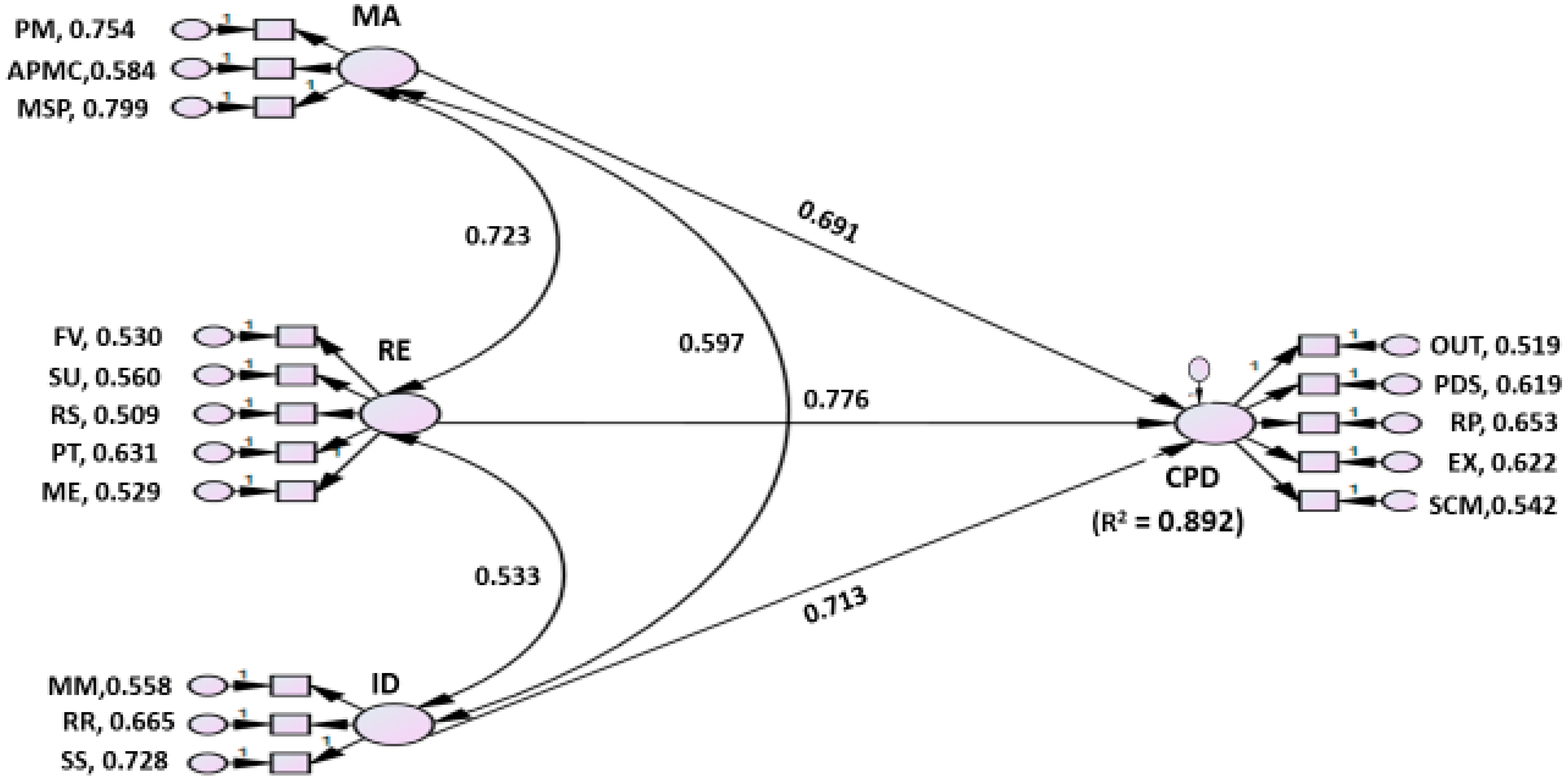
• The findings of the measurement model inferred that the factor loadings of all the indicators across the RE, ID, and MA exogenous variables are significant in influencing the CPD. To be more precise, the PT, MSP, and SS indicators received the highest loading factors for the RE, MA, and ID exogenous variables, respectively. Therefore, enhanced production and release of high-yielding chickpea varieties from informal sources such as non-government organizations, FPOs, and progressive farmers; linking cold storage systems and warehouses to e-NAM; extending loans to FPOs from AIF to strengthen storage structures and processing facilities; linking farmers to markets, etc., deserve special attention towards CPD.
• Similarly, the RP indicator received the highest loading factor in the endogenous variable, CPD. Therefore, in the long run, the selected states should focus on sustainable growth of chickpeas that is also financially sustainable. To ensure this, there should be flexibility in the intervention price, and prices should be allowed to move up and down in response to changes in the market conditions. The pricing mechanism and policy should offer considerable margins levels over production costs to chickpea farmers.
• The exogenous variable RE exerted the strongest influence on CPD with a direct effect of 0.776, followed by the ID and MA variables with direct effects of 0.713 and 0.691, respectively. These three exogenous variables cumulatively explained 89 percent of the total variation in CPD. Therefore, the findings from this research have shown that the determined model has perfect fit.
• All the three constructs, viz., MA, RE, and ID, had positive and significant indirect effects on the OUT, PDS, RP, EX, and SCM indicator variables of the CPD. Further, these three constructs showed the highest and most significant indirect impact on the RP indicator of the endogenous variable.
• The hypotheses formulated between the exogenous variables and endogenous variable are supported through SEM.
• Finally, the study has emphasized that in the selected states, the respective governments should assign relatively more importance to the RE, ID, and MA constructs and accordingly should focus on the PT, SS, and MSP indicators, respectively, on a priority basis for promoting CPD in the ensuing future.

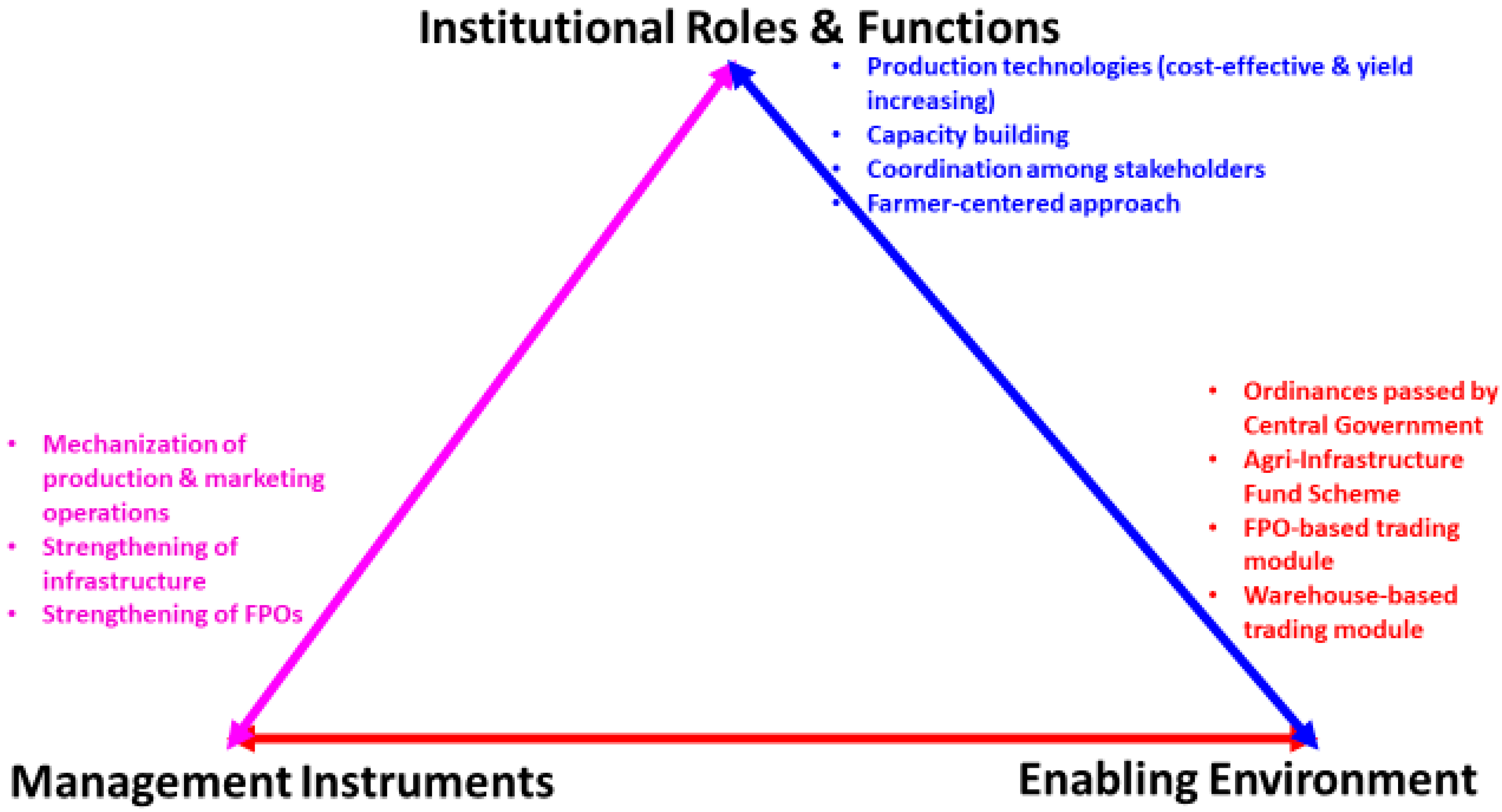
The recommended policy guidelines are as follows: Popularization of cost-effective production technologies, promotion of FPOs, strengthening of cold storage structures and warehouses and linking them to e-NAM, and effective implementation of MSP policy deserve special attention in the future. Though the empirical results provide evidence of positive impacts of RE, ID, and MA and their corresponding indicator variables on CPD, the main contributions of the present study, however, reside in the relationship between the PT, SS, and MSP indicators of RE, ID, and MA, respectively, on a priority basis for promoting CPD in the ensuing future. Therefore, it is high time to assign relative importance to the R&D of cost-effective production technologies, strengthening of storage structures to overcome distress sales of produce, and announcing higher MSP to encourage farmers to opt for chickpea cultivation on a large scale. With India being a net importer of pulses in general and chickpeas in particular, the role of the state should be extensive in focusing on the above three indicators. Interestingly, across all the selected states, the enabling environment is very much favorable towards popularizing chickpea cultivation (Figure 4). Even the institutional roles and functions and management instruments ensure a positive picture to realize the true benefits of practicing chickpea cultivation. Therefore, this policy should be viewed from a broader perspective to further gear up both production and marketing reforms. However, the fruits of these reforms can be better realized in the near future if the state governments develop their own contextualized strategies and popularize them among chickpea farmers and other stakeholders.

However, this study has a few limitations that should be addressed in future research. First, this study is focused on CPD in three major chickpea-cultivating states, viz., Madhya Pradesh, Rajasthan, and Maharashtra, in India and is aimed at prioritizing exogenous variables and their respective indicator variables. To confirm the validity of this model, future research should examine this model as a conceptual framework in other states and even for other crops. Second, this study was conducted in only three states, and therefore it is not possible to generalize the findings to other chickpea-cultivating states. Third, future research employing time series or panel data should be considered to ascertain the extent of implementation of policy mechanisms that contribute to long-term CPD in India. Finally, future research should consider the preferences of both farmers and consumers for the attributes in chickpea varieties that promote CPD in the study area.

References

1. FAO. Crops and Livestock Products. Available online: http://www.fao.org/faostat/en/#data/QCL (accessed on 6 February 2021).
2. Pulse POD. Available online: https://pulsepod.globalpulses.com (accessed on 6 February 2021).
3. Tiwari, A.K.; Shivhare, A.K. Pulses in India—Retrospect and Prospects—Government of India; Ministry of Agriculture; Department of Agriculture and Cooperation; Directorate of Pulses Development: Bhopal, India, 2016.
4. Agricultural Statistics at a Glance, Various Issues; Ministry of Agriculture and Farmers’ Welfare; Government of India: Bhopal, India, 1951–2019.
5. The Big Picture, Why India Needs to Focus More on Production of Pulses at Home. Available online: https://yourstory.com (accessed on 7 July 2021).
6. FAO. Food Loss Analysis: Causes and Solutions—Case Study on the Chickpea Value Chain in the Republic of India; Food and Agriculture Organization: Rome, Italy, 2018; p. 52. [Google Scholar]
7. Asadi, A.; Kalantari, K.; Choobchian, S. Structural analysis of factors affecting agricultural sustainability in Qazvin Province, Iran. J. Agric. Sci. Technol. 2013, 15, 11–22. [Google Scholar]
8. Rohaeni, E.S.; Hartono, B.; Fanani, Z.; Nugroho, B.A. Sustainability of cattle farming using analysis approach of Structural Equation Modeling (a study on dry land of Tanah Laut Regency, South Kalimantan, Indonesia). Int. J. Agron. Agric. Res. 2014, 4, 8–21. [Google Scholar]
9. Yasar, M.; Siwar, C.; Firdaus, R.R. Assessing paddy farming sustainability in the Northern Terengganu Integrated Agricultural Development Area (IADA KETARA): A structural equation modelling approach. Pac. Sci. Rev. B Humanit. Soc. Sci. 2015, 1, 71–75. [Google Scholar] [CrossRef] [Green Version]
10. Fatemi, M.; Azadi, H.; Rafiaani, P.; Taheri, F.; Dubois, T.; Van Passel, S.; Witlox, F. Effects of Supply Chain Management on Tomato Export in Iran: Application of Structural Equation Modeling. J. Food Prod. Mark. 2018, 24, 177–195. [Google Scholar] [CrossRef]
11. Yontar, E.; Ersöz, S. Investigation of Food Supply Chain. Sustainability Performance for Turkey’s Food Sector. Front. Sustain. Food Syst. 2020, 4, 1–21. [Google Scholar] [CrossRef]
12. Baruwadi, M.H.; Akib, F.H.Y.; Bahua, M.I. Impact of Agricultural Extension Performance on Corn Farmers Household Economy. J. Austrian Soc. Agric. Econ. 2020, 16, 137–146. [Google Scholar]
13. Kothari, C.R. Research Methodology: Methods and Techniques, 2nd ed.; New Age International Limited: New Delhi, India, 2014; p. 179. [Google Scholar]
14. Werner, C.; Schermelleh-Engel, K. Structural Equation Modeling: Advantages, Challenges, and Problems; Goethe University: Frankfurt, Germany, 2009. [Google Scholar]
15. Bollen, K.A. Structural Equations with Latent Variables; John Wiley & Sons: New York, NY, USA, 1989; Volume 29. [Google Scholar]
16. Fornell, C.; Larcker, D.F. Evaluating structural equation models with unobservable variables and measurement error. J. Mark. Res. 1981, 48, 39–50. [Google Scholar] [CrossRef]
17. Joreskog, K.G.; Sorbom, D. LISREL 8: User’s Reference Guide; Scientific Software International, Inc.: Chicago, IL, USA, 1996; Volume 4, p. 43. [Google Scholar]
18. Sanchez, G.M.; Nejadhashemi, A.P.; Zhang, Z.; Marquart-Pyatt, S.; Habron, G.; Shortridge, A. Linking watershed-scale stream health and socioeconomic indicators with spatial clustering and structural equation modeling. Environ. Model. Softw. 2015, 70, 113–127. [Google Scholar] [CrossRef]
19. Hair, J.F.; Black, W.C.; Basin, B.J.; Person, R.E. Multivariate Data Analysis, 7th ed.; Pearson Prentice Hall: Upper Saddle River, NJ, USA, 2010. [Google Scholar]
20. Lubis, R. Sustainable Agriculture Development Using Structural Equation Model Approach (Case Study of Simalungun Regency—Indonesia). Int. J. Recent Sci. Res. 2017, 8, 21029–21035. [Google Scholar]
21. Schumacker, R.E.; Lomax, R.G. A Beginner’s Guide to Structural Equation Modelling; Psychology Press, Routledge, Taylor & Francis Group: New York, NY, USA, 2004. [Google Scholar]
22. Sekaran, U. Research Methods for Business; Wiley & Sons, Inc.: New York, NY, USA, 2003. [Google Scholar]
23. Sevilla, C.G. Pengantar Metode Penelitian; UI Press: Jakarta, Indonesia, 1993. [Google Scholar]
24. Amos, L.d.; Solimun, M.S. Structural Equation Modeling (SEM); Malang University: Malang, Indonesia, 2002. [Google Scholar]
25. Suhr, D.D. Exploratory or Confirmatory Factor Analysis? Cary SAS Institute: Cary, NC, USA, 2006; pp. 1–17. [Google Scholar]
26. Kaiser, H.F. An index of factorial simplicity. Psychometrika 1974, 39, 31–36. [Google Scholar] [CrossRef]
27. Magrini, A.; Bartolini, F.; Coli, A.; Pacini, B. A structural equation model to assess the impact of agricultural research expenditure on multiple dimensions. Qual. Quant. 2019, 53, 2063–2080. [Google Scholar] [CrossRef]
28. Rahmaninkoshkaki, M.; Zarei, Y. Designing the Structural Equation Model of Agricultural Entrepreneurship Development in Rural Areas of Iran (Case Study: Villages of Marvdasht County). Int. J. Agric. Sci. Res. Technol. Ext. Educ. Syst. 2018, 8, 17–27. [Google Scholar]
29. Field, A. Discovering Statistics Using SPSS; Sage Publications: New York, NY, USA, 2009. [Google Scholar]
30. Juhary, A.; Ilham, S. The mediating effect of good governance on the relationship between managerial roles and personal development: A Structural Equation Modeling (SEM) approach. J. US-China Public Adm. 2008, 5, 1–15, ISSN 1548-6591. [Google Scholar]
31. Correia, L.; El-Ahmadi, A.; Molle, B.; Maia, R.; Oliveira, I. Benchmark irrigation practices on olives using a Structural Equation Modelling approach. Irrig. Drain. 2012, 61, 189–200. [Google Scholar] [CrossRef]
32. Gruda, M.; Kwasek, M.; Rembisz, W. Structural Equation Modeling in Research of Sustainable Agriculture. In Proceedings of the EcoMod2012, Seville, Spain, 4–6 July 2012; Volume 4567, pp. 1–12. [Google Scholar]
33. Harijati, S. Potencies and Development of Smallholders’ Agribusiness Competency: A Case of Vegetable Farmers in the City and Outskirt of Jakarta and Bandung. Ph.D. Thesis, Agricultural University, Bogor, Indonesia, 2007. (In Indonesian). [Google Scholar]
34. Sentosa, I.; Bambang, B.S.; Ming, C.W.M.C.W.; Kamaria, N.K.N.M. A Structural Equation Modeling of internet banking usage in Malaysia. J. Arts Sci. Commer. 2012, 3, 75–86. [Google Scholar]
35. Ankamah, J.; Kodua, T.T.; Addae, M. Structural equation modelling of perception for sustainable agriculture as climate change mitigation strategy in Ghana. Environ. Syst. Res. 2021, 10, 1–13. [Google Scholar] [CrossRef]
36. Nacife, J.M.; Soares, F.A.L.; Teixeira, M.B.; dos Santos, L.N.S.; Castoldi, G. Structural Equation Modeling Applied to Socioeconomic Indicators in the Production of Sugarcane, in the State of Goiás. Int. J. Bus. Adm. 2019, 10, 53–64. [Google Scholar]
37. Hatta Jamil, M.; Jahi, A.; Arsyad, M.; Sarma, M.; Gusti Putu Purnaba, I.; Viantika, N.M.; Rachmawaty, A.; Nadja, A.; Tenriawaru, N.; Bahua, M.I. Determinants Factors of Agricultural Extension Services Performance and Impacts on Farmers’ Behavior. Am. J. Agric. Biol. Sci. 2017, 12, 33–38. [Google Scholar] [CrossRef]
38. Neville, N.; Godfrey, S.; Njimanted, F.; Thalut, N.; Yildiz, F. Effect of farmers’ management practices on safety and quality standards of cocoa production: A structural equation modeling approach. Food Sci. Technol. Cogent Food Agric. 2020, 6, 1844848. [Google Scholar]
39. Gaur, P.M.; Tripathi, S.; Gowda, C.L.L.; Ranga Rao, G.V.; Sharma, H.C.; Pande, S.; Sharma, M. Chickpea Seed Production Manual; International Crops Research Institute for the Semi-Arid Tropics: Andhra Pradesh, India, 2010; p. 28. [Google Scholar]
40. John, J.; Bhatt, A.; Varma, P. Impact of Minimum Support Price Policy and National Food Security Mission on the Production of Pulses in India. In Proceedings of the Agricultural & Applied Economics Association Annual Meeting, Atlanta, GA, USA, 21–23 July 2019. [Google Scholar]
41. Henseler, J.; Ringle, C.M.; Sarstedt, M. A New Criterion for Assessing Discriminant Validity in Variance-Based Structural Equation Modeling. J. Acad. Mark. Sci. 2015, 43, 115–135. [Google Scholar] [CrossRef] [Green Version]
42. Nejatian, H.; Piaralal, S.K.; Sentosa, I.; Bohari, A.M. The Influence of Customer Knowledge on CRM Performance of Malaysian ICT Companies: A Structural Equation Modeling Approach. Int. J. Bus. Manag. 2011, 6, 181–198. [Google Scholar] [CrossRef] [Green Version]
43. Paswan, A. Confirmatory Factor Analysis and Structural Equations Modeling, An Introduction; Department of Marketing and Logistics, COB; University of North Texas: Denton, TX, USA, 2009. [Google Scholar]
44. Daire, H.; Joseph, C.; Michael, R.M. Structural Equation Modeling: Guidelines for Determining Model Fit. Electron. J. Bus. Res. Methods 2008, 6, 53–60. [Google Scholar]
45. Hu, L.T.; Bentler, P.M. Cutoff Criteria for Fit Indexes in Covariance Structure Analysis: Conventional Criteria versus New Alternatives. Struct. Equ. Model. 1999, 6, 1–55. [Google Scholar] [CrossRef]
46. Najafabadi, M.O. Gender Sensitive Analysis towards Organic Agriculture: A Structural Equation Modeling Approach. J. Agric. Environ. Ethics 2014, 27, 225–240, ISSN 1187-7863. [Google Scholar] [CrossRef]
47. Kumari, M.; Singh, R. Production and Marketing of Chickpea in Bihar: Problems and Prospects for the farmers. Int. J. Agric. Sci. Res. 2016, 6, 125–136. [Google Scholar]
Figure 1. (a) Global scenario of chickpea area during TE 2019; (b) Global scenario of chickpea production during TE 2019.
Sustainability 13 10283 g001
Figure 2. Operational model of interventions for CPD in India.
Sustainability 13 10283 g002
Figure 3. Structural model parameter estimation for CPD in India.
Sustainability 13 10283 g003
Figure 4. Broader areas to popularize chickpea cultivation in India.
Sustainability 13 10283 g004