Optimal Procurement Strategy for Supply Chain with Trade Credit and Backorder under CVaR Criterion

Abstract

Some capital-constrained and risk-averse retailers may unable to obtain financing from banks due to insufficient collateral and high loan costs, so some retailers tend to use trade credit financing to ease their financial pressure. For the two echelon supply chain composed of a well-funded supplier and a capital-constrained retailer with risk-averse preference, a trade credit strategy model with the supplier-led is established in this paper. By analyzing both parties’ benefits, we derive the model solution and provide optimal decisions to all petitioners. The results obtained in this paper show that the optimum order quantity under the Conditional Value-at-Risk (CVaR) criterion declines w.r.t. the confidence level, and the wholesale price of the supplier increases w.r.t. the confidence level. The reason is that when the retailer makes fewer orders, the supplier will correspondingly increase the wholesale price to maximize their profit. On the other hand, the ordering policy with allowing backorder will make the retailer place fewer orders. Finally, the proposed model is indicated by the given numerical experiments.

1. Introduction

Many enterprises face fundamental problems affecting decision-making, such as high operation risk, supply shortage, financial constraints, and so on. The capital-constrained enterprises often need to use financing to alleviate financial pressure and maintain the company’s regular operation. Due to the difficulty of bank credit financing, capital-constrained enterprises may choose the trade credit strategy. At the same time, many enterprises tend to offer the retailer a trade credit to stimulate the retailer make a larger order to reduce the order processing cost. In other words, they allow their retailer to defer payment for the purchase for some time [1,2]. From the data of the Federal Reserve Board of the United States (2019), the amount of trade credit transactions increased by 17.77% in 2018 compared with the past. This policy received much attention from researchers, see, e.g., Haley and Higgins [3], Jamal et al. [4] and Jaggi et al. [5], Arcelus and Srinivasan [6], Huang [7], Chung [8] and Wang et al. [9], Schwartz [10] and references therein.

For the supply chain with trade credit model, Kouvelis et al. [11] showed that both the supplier’s benefit and supply chain can be significantly improved and the retailer profits is improved under optimal trade credit contracts relative to that under bank financing. Jing et al. [12] showed that when bank credit and trade credit exist simultaneously, trade credit will be the only equilibrium strategy when the production cost is relatively low. Deng et al. [13] showed that if one retailer runs the bankruptcy risk due to the provided trade credit, other retailers would alter their competition behaviour and the profit thus would not be the same. Chen et al. [14] found that the trade credit provided by suppliers increases the profits of both sides and reduces the default risk of retailers. The other literature for inventory models with trade credit include Chod [15], Houston et al. [16], Lei et al. [17], An et al. [18], Chen et al. [14], Das et al. [19].

Due to the financial crisis in recent decades, the risk aversion of enterprises has been significantly received much attention. For example, enterprises become more risk averse in making decisions in response to the instability of the US dollar exchange rate and the turbulence caused by the trade war [20]. Therefore, it is feasible to introduce the risk aversion of supply chain members into the trade credit model. Due to the randomness of the demand, to reduce the influence of the volatile market and the ensuing losses, some researchers consider the risk analysis and risk control from the retailer’s perspective. For this, Wang [21] addressed the newsvendor model with loss aversion, and Qiu et al. [22] considered the robust inventory model from the perspective of risk-averse managers given incomplete demand data of the market. Choi et al. [23] revealed that a Pareto improving optimal measure would be achieved with risk-netural participants within the supply chain and unlikely inappropriately significantly increase in production cost. Song et al. [24] showed that the number of products would become smaller and the profit of the engagers falls owing to the supplier’s risk aversion under the pull strategy. For related researches see, e.g., [25,26,27,28,29,30,31,32,33,34,35,36].

A shortage in market activities is inevitable. Due to the existence of shortages, some customers choose to buy a substitute, and some customers choose to backorder, i.e., the customers wait for the merchant to supplement and then purchase the products. Plenty of studies have probed into the newsvendor model with backorder [36,37,38,39,40,41].

In reality, trade credit, backorder and risk aversion tend to coexist. Thus, the research on the optimal strategy for supply chain with trade credit, backorder and risk preference suggests many practical values, which constitutes the paper’s motivation. More precisely, in this paper, we will consider the two-echelon supply chain with trade credit under the CVaR criterion by providing the optimal policy of both parties when the retailer is capital-constrained and risk-averse, analyzing the affect of the retailer’s risk aversion on the decision of both parties and the impact on the retailer’s order quantity with backorder. To this end, a two-echelon supply chain comprising a well-funded supplier as well as a capital-constrained retailer with risk-averse preference is established. In particular, this paper establishes a strategy model with trade credit under CVaR criterion. By analyzing benefits of both the supplying and the retailing sides, we obtain the suppliers’ and retailers’ optimal decisions, respectively. Finally, the proposed model is indicated by the given numerical experiments.

The remainder of this paper is arranged as follows. Section 2 describes the general model and presents notations as well as necessary assumptions. Section 3 considers the equilibrium of supply chain parties under trade credit policy. Numerical experiments are carried out in Section 4. Section 5 gives conclusions and some remarks.

2. Problem Description and Notation

Consider a supply chain consists of a supplier with sufficient funding and a retailer with limited capital. As the start, the supplier sets a wholesale price for the retailer and proposes a trade credit strategy as well. With this, the retailer should determine how many goods to order by considering their initial cash flow to meet stochastic demand. Due to funding constraints, the retailer may adopt the trade credit strategy or use only their capital at the starting point if it is sufficient. Further, if there are funds left after paying for the order, the retailer may invest it for risk-free interests. On the other hand, if the retailer accepts the trade credit strategy, he can make a partial pay for the order with the initial funds, and the supplier should get the payment arrears and interest of the trade credit at the end. To maximize their own benefit, the supplier should choose a wholesale price that suits them so well that the retailer can place a larger order. Moreover, the retailer would determine their ordering quantity according to their initial funds, and the wholesale price and the trade credit strategy provided by the supplier. This constitutes a supplier-led Stackelberg game.

For the related model, since the demand at each replenishment cycle is random, there is the risk of loss for any order. Hence, the retailer should take their attitude to the risk of loss into consideration when ordering. The prerequisite assumes that the retailer would manage to make risk-averse choices. To solve the model, we need some notations and some assumptions (see

Table 1. Notations.

Symbol	Description
Q	retailer’s order quantity
w	unit wholesale price
$y_0$	retailer’s initial cash flow
b	retailer’s selling price per unit
c	supplier’s production cost per unit
f	retailer’s backorder cost per unit
$r_s$	supplier’s interest rate
$r_f$	risk-free interest rate
$\epsilon$	retailer’s salvage value of unit unsold product
$\tau$	confidence level of retailer (0 < $\tau$ < 1)
$\eta$	retailer’s backorder rate (0 < $\eta$ < 1)

).

Assumption 1.

The supplier is neutral while the retailer is averse towards risks. The retailer faces capital constraints, while the supplier is well funded.

Assumption 2.

The market demand D is random with the probability density function $f(x)$ and cumulative distribution function $F(x)$.

Assumption 3.

When the retailer is out of stock, the retailer makes emergency replenishment to the same type of enterprise nearby rather than the supplier.

For the parameters involved in the model, we further assume that $r_s>r_f$ and $b>f>w(1+r_s)>w(1+r_f)>c>\epsilon >0$.

3. The Model of Supply Chain with Trade Credit

The running pattern of the relevant model is as follows: the supplier first sets a wholesale price w and provides a trade credit with interest strategy to the retailer, and the retailer determines their ordering quantity Q. Because the scale of suppliers is usually large and have much information, the supplier is the leader in the Stackelberg game. If the ordering cost is less than the retailer’s initial cash flow, then the retailer would use their initial cash flow to pay the order and invest the remaining fund to earn a risk-free interest. Otherwise, the retailer would adopt the trade credit policy to pay for the order. In the case above, the supplier can earn risk-free interest on the received payment. If the retailer chooses the trade credit strategy, the supplier will obtain interest income at the end of the period. Indeed, the supplier needs to determine the wholesale price w to maximize their profit, and the retailer determines the order quantity based on their initial cash flow $y_0$ and the wholesale price w to maximize their profit, this constitutes a Stackelberg model. To solve the model, we first consider the retailer’s decision according to the fixed wholesale priced by the supplier, and then caculate the wholesale price w to maximize the supplier’s profit based on the retailer’s optimal decision. At this time, the Stackelberg equilibrium is reached.

For the related model, for the fixed wholesale price, the retailer would choose their initial funds to pay for the order if he can afford it by their initial fund. That is, for the order Q(decision variables), if $wQ<y_0$, the retailer would use their initial cash flow to pay for the order and invest the remaining fund $(y_0-wQ)$ to earn a risk-free interest ${(y_0-wQ)}^{+}{r}_f$, where ${(·)}^{+}$ means the maximum of the scaler and zero. Otherwise, $wQ>y_0$, and the retailer would use their initial fund and accept the trade credit policy. The for order quantity Q, the retailer can obtain gross profit $bmin(Q,D)$ and recovery profit $\epsilon {(Q-D)}^{+}$ for order Q. We set the backorder rate to be $\eta$ and the retailer’s unit backorder cost to be f. At this point, the benefit of backorder is $\eta (b-f){(D-Q)}^{+}$. Consequently, the retailer’s profit in one replenishment cycle can be computed as

$$\pi (Q)=bmin(Q,D)-wQ+{(y_0-wQ)}^{+}{r}_f-{(wQ-y_0)}^{+}{r}_s+\epsilon {(Q-D)}^{+}+\eta (b-f){(D-Q)}^{+}.$$

(1)

The supplier’s decision variable is the wholesale price w. When the retailer’s initial funds are sufficient to pay the ordering expenses or only use all its funds to buy products, the supplier can make the risk-free investment $(w-c)Q{r}_f$ on the remaining payment. At this time, the supplier’s profit function is in Equation (2). When the retailer’s initial capital is insufficient to pay the ordering and adopt the trade credit strategy, the supplier will receive the retailer’s initial capital for risk-free investment $y_0{r}_f$ and charge interest income $(wQ-y_0)r_s$ at the end of the period. At this time, the supplier’s profit function is in Equation (3).

$$\Pi (w)=(w-c)Q(1+r_f).$$

(2)

$$\Pi (w)=(w-c)Q+y_0{r}_f+(wQ-y_0)r_s.$$

(3)

Due to the risk of loss in the replenishment cycle, the retailer has some preference when making decisions. To characterize the behavior preference of the retailer, we adopt CVaR theory introduced by Kahneman and Tversky [42,43].

The CVaR criterion can be seen as a downsize risk criterion which focus more on the loss exceeding a given target level, or in other words, the benefit not satisfying a given target level. This term is widely used for risk control by the retailer who in this model is assumed to be risk-averse [25,44]. Usually, the VaR about the benefit $\pi (Q)$ for the risk-averse retailer is defined as

$${VaR}_{\tau }[\pi (Q)]=sup[\phi \in R\mid Pr[\pi (Q)⩾\phi ]⩾\tau ],$$

where $Pr[\pi (Q)⩾\phi ]$ indicates the probability of the benefit $\pi (Q)$ above value $\phi$, and ${VaR}_{\tau }[\pi (Q)]$ means the maximum benefit of the retailer who has been set risk-averse at the confidence level $\tau$. Using ${VaR}_{\tau }[\pi (Q)]$ to denote the targeted benefit, the CVaR about benefit $\pi (Q)$ going to the retailer can now be defined as

$${\mathrm{CVaR}}_{\tau }[\pi (Q)]=\frac{1}{1-\tau }E[\pi (Q)\mid \pi (Q)⩽{VaR}_{\tau }[\pi (Q)]].$$

By maximizing this CVaR criterion, i.e., solving the optimization problem

$$max{\mathrm{CVaR}}_{\tau }[\pi (Q)]=\frac{1}{1-\tau }E[\pi (Q)\mid \pi (Q)⩽{VaR}_{\tau }[\pi (Q)]]$$

(4)

Since the problem is difficult to solve and it is usually transformed into the following equivalent optimization problem [44]

$$\underset{Q,\phi }{max}{H}_{\tau }(Q,\phi )=\phi -\frac{1}{1-\tau }E{(\phi -\pi (Q))}^{+}.$$

(5)

Based on this, the following conclusion for the problem is thus obtained.

Theorem 1.

For $\tau \in (0,1)$, for the early set wholesale price, the best ordering number for the retailer in the concerned model is such that

$$Q^{*}=\left[\begin{array}{cc}& F{\left(\frac{(1-\tau )[b-\eta (b-f)-w(1+r_s)]}{b-\epsilon -\eta (b-f)}\right)}^{-1},\mathrm{if}\frac{y_0}{w}\in \left(0,F{\left(\frac{(1-\tau )[b-\eta (b-f)-w(1+r_s)]}{b-\epsilon -\eta (b-f)}\right)}^{-1}\right],\hfill \\ & \frac{y_0}{w},\mathrm{if}\frac{y_0}{w}\in \left(F{\left(\frac{(1-\tau )[b-\eta (b-f)-w(1+r_s)]}{b-\epsilon -\eta (b-f)}\right)}^{-1},F{\left(\frac{(1-\tau )[b-\eta (b-f)-w(1+r_f)]}{b-\epsilon -\eta (b-f)}\right)}^{-1}\right),\hfill \\ & F{\left(\frac{(1-\tau )[b-\eta (b-f)-w(1+r_f)]}{b-\epsilon -\eta (b-f)}\right)}^{-1},\mathrm{if}\frac{y_0}{w}\in \left[F{\left(\frac{(1-\tau )[b-\eta (b-f)-w(1+r_f)]}{b-\epsilon -\eta (b-f)}\right)}^{-1},\infty \right).\hfill \end{array}\right.$$

Proof. 

To find the solution to (5), this paper will discuss the problem in two cases: one where the risk-averse retailer needs to make a trade credit, and one where they do not.

Case 1. The risk-averse retailer does not use the trade credit, i.e., $wQ-y_0⩽0$. Then for order Q, using the fact that $min[Q,D]=Q-{(Q-D)}^{+}$ and ${(D-Q)}^{+}=D-Q+{(Q-D)}^{+}$, one has

$$\begin{array}{cc}\hfill \pi (Q)=& bmin(Q,D)-wQ+(y_0-wQ)r_f+\epsilon {(Q-D)}^{+}+\eta (b-f){(D-Q)}^{+}\hfill \\ \hfill =& (b-w-\eta (b-f))Q+\eta (b-f)D+r_f(y_0-wQ)-(b-\epsilon -\eta (b-f)){(Q-D)}^{+}.\hfill \end{array}$$

(6)

Then the objective function of problem (5) can be written as

$$\begin{array}{cc}\hfill H_{\tau }(Q,\phi )=& \phi -\frac{1}{1-\tau }E{(\phi -\pi (Q))}^{+}\hfill \\ \hfill =& \phi -\frac{1}{1-\tau }{\int }_0^{+\infty }\left[\phi -(b-w-\eta (b-f))Q-\eta (b-f)x\right.\hfill \\ \hfill & {\left.-r_f(y_0-wQ)+(b-\epsilon -\eta (b-f)){(Q-x)}^{+}\right]}^{+}\mathrm{d}F(x)\hfill \\ \hfill =& \phi -\frac{1}{1-\tau }{\int }_0^Q{\left[\phi -\epsilon Q+wQ-(b-\epsilon )x-r_f(y_0-wQ)\right]}^{+}\mathrm{d}F(x)\hfill \\ \hfill & -\frac{1}{1-\tau }{\int }_Q^{+\infty }{\left[\phi -(b-w-\eta (b-f))Q-\eta (b-f)x-r_f(y_0-wQ)\right]}^{+}\mathrm{d}F(x).\hfill \end{array}$$

(7)

To solve the problem, we first consider the inner problem, i.e.,

$$\underset{\phi }{max}{H}_{\tau }(Q,\phi )$$

for fixed Q in two subcases.

Subcase 1.1. $\phi <bQ-wQ+r_f(y_0-wQ).$ Under this circumstance, given Equation (7), we obtain

$$\begin{array}{cc}\hfill H_{\tau }(Q,\phi )=& \phi -\frac{1}{1-\tau }{\int }_0^{\frac{\phi -\epsilon Q+wQ-r_f(y_0-wQ)}{b-\epsilon }}\left[\phi -\epsilon Q+wQ\right.\hfill \\ & \left.-(b-\epsilon )x-r_f(y_0-wQ)\right]\mathrm{d}F(x),\hfill \end{array}$$

and

$$\frac{\partial H(Q,\phi )}{\partial \phi }=1-\frac{1}{1-\tau }F\left(\frac{\phi -\epsilon Q+wQ-r_f(y_0-wQ)}{b-\epsilon }\right).$$

Certainly,

$${\left.\frac{\partial H(Q,\phi )}{\partial \phi }\right|}_{\phi =\epsilon Q-wQ+r_f(y_0-wQ)}=1>0.$$

Thus, if

$${\left.\frac{\partial H(Q,\phi )}{\partial \phi }\right|}_{\phi =bQ-wQ+r_f(y_0-wQ)}=1-\frac{1}{1-\tau }F(Q)⩽0,$$

namely, $Q⩾F^{-1}(1-\tau )$, then problem ${max}_{\phi ⩾0}H(Q,\phi )$ has the optimal solution that is its stationary point, which means that

$$\begin{array}{c}\hfill {\phi }^{*}=(b-\epsilon )F^{-1}(1-\tau )-wQ+\epsilon Q+r_f(y_0-wQ).\end{array}$$

On the other hand, if

$${\left.\frac{\partial H(Q,\phi )}{\partial \phi }\right|}_{v=bQ-wQ+r_f(y_0-wQ)}=1-\frac{1}{1-\tau }F(Q)>0,$$

then function $H(Q,\phi )$ is increasing w.r.t. $\phi$, and it collapses to the next subcase.

Subcase 1.2. $\phi ⩾bQ-wQ+r_f(y_0-wQ)$. In this subcase, it can be concluded from Equation (7) that

$$\begin{array}{cc}\hfill H_{\tau }(Q,\phi )=& \phi -\frac{1}{1-\tau }{\int }_0^Q[\phi -\epsilon Q+wQ-(b-\epsilon )x-r_f(y_0-wQ)]\mathrm{d}F(x)\hfill \\ & -\frac{1}{1-\tau }{\int }_Q^{\frac{\phi -(b-w-\eta (b-f))Q-r_f(y_0-wQ)}{\eta (b-f)}}[\phi -(b-w-\eta (b-f))Q\hfill \\ & -\eta (b-f)x-r_f(y_0-wQ){]}^{+}\mathrm{d}F(x),\hfill \end{array}$$

and

$$\frac{\partial H(Q,\phi )}{\partial \phi }=1-\frac{1}{1-\tau }F\left(\frac{\phi -(b-w-\eta (b-f))Q-r_f(y_0-wQ)}{\eta (b-f)}\right).$$

Then a sufficiently large ${\phi }_0$ exists such that

$$\frac{\partial H(Q,\phi )}{\partial \phi }{|}_{\phi ={\phi }_0}=1-\frac{1}{1-\tau }F\left(\frac{{\phi }_0-(b-w-\eta (b-f))Q-r_f(y_0-wQ)}{\eta (b-f)}\right)⩽0.$$

If

$$\frac{\partial H(Q,\phi )}{\partial \phi }{|}_{\phi =bQ-wQ+r_f(y_0-wQ)}=1-\frac{1}{1-\tau }F(Q)>0,$$

i.e., $Q<F^{-1}(1-\tau ),$ then problem ${min}_{\phi ⩾0}H(Q,\phi )$ has its optimal solution ${\phi }^{*}$ which satisfies that

$$1-\frac{1}{1-\tau }F\left(\frac{\phi -(b-w-\eta (b-f))Q-r_f(y_0-wQ)}{\eta (b-f)}\right)=0,$$

which means that

$${\phi }^{*}=\eta (b-f)F^{-1}(1-\tau )+(b-w-\eta (b-f))Q+r_f(y_0-wQ).$$

Otherwise,

$$\frac{\partial H(Q,\phi )}{\partial \phi }{|}_{\phi =bQ-wQ+r_f(y_0-wQ)}=1-\frac{1}{1-\tau }F(Q)<0,$$

and function $H(Q,\phi )$ is decreasing w.r.t. $\phi$, which collapses to subcase 1.1.

Based on the discussion above, the optimum solution can be obtained for arbitrary fixed Q to ${min}_{\phi ⩾0}H(Q,\phi )$

$${\phi }^{*}=\left[\begin{array}{cc}(b-\epsilon )F^{-1}(1-\tau )+\epsilon Q-wQ+r_f(y_0-wQ),\hfill & \mathrm{if}Q⩾F^{-1}(1-\tau ),\hfill \\ \eta (b-f)F^{-1}(1-\tau )+(b-w-\eta (b-f))Q+r_f(y_0-wQ),\hfill & \mathrm{if}Q<F^{-1}(1-\tau ).\hfill \end{array}\right.$$

(8)

Now, we turn to considering the outer problem of the problem ${max}_{Q⩾0}{max}_{\phi ⩾0}H(Q,\phi )$, i.e., solving ${max}_{Q⩾0}H(Q,{\phi }^{*}).$ For this, we similarly break the discussion into two subcases.

Subcase 2.1. $Q⩾F^{-1}(1-\tau )$. Under this circumstance, from the fact that

$${\phi }^{*}=(b-\epsilon )F^{-1}(1-\tau )+\epsilon Q-wQ+r_f(y_0-wQ),$$

we conclude that the objective function $H(Q,{\phi }^{*})$ can be written as

$$\begin{array}{cc}\hfill H(Q,{\phi }^{*})=& (b-\epsilon )F^{-1}(1-\tau )+\epsilon Q-wQ+r_f(y_0-wQ)\hfill \\ & -\frac{1}{1-\tau }{\int }_0^{F^{-1}(1-\tau )}[(b-\epsilon )(F^{-1}(1-\tau )-x)]\mathrm{d}F(x).\hfill \end{array}$$

Since

$$\frac{\partial H(Q,{\phi }^{*})}{\partial Q}=\epsilon -w(1+r_f)<0,$$

its maximum can be reached in the interval $(0,F^{-1}(1-\tau )).$

Subcase 2.2. $Q<F^{-1}(1-\tau )$. Under this circumstance,

$${\phi }^{*}=\eta (b-f)F^{-1}(1-\tau )+(b-w-\eta (b-f))Q+r_f(y_0-wQ).$$

Hence,

$$\begin{array}{cc}\hfill H(Q,{\phi }^{*})=& \eta (b-f)F^{-1}(1-\tau )+(b-w-\eta (b-f))Q+r_f(y_0-wQ)\hfill \\ & -\frac{1}{1-\tau }{\int }_0^Q[\eta (b-f)F^{-1}(1-\tau )+(b-\epsilon -\eta (b-f))Q-(b-\epsilon )x]\mathrm{d}F(x)\hfill \\ & +\frac{1}{1-\tau }{\int }_Q^{F^{-1}(1-\tau )}[\eta (b-f)(F^{-1}(1-\tau )-x)]\mathrm{d}F(x),\hfill \end{array}$$

and

$$\frac{\partial H(Q,{\phi }^{*})}{\partial Q}=b-\eta (b-f)-w(1+r_f)-\frac{1}{1-\tau }(b-\epsilon -\eta (b-f))F(Q).$$

(9)

The optimal solution Q is then obtained to solve problem ${max}_{Q⩾0}H(Q,{\phi }^{*})$, i.e.,

$$Q=F{\left(\frac{(1-\tau )[b-\eta (b-f)-w(1+r_f)]}{b-\epsilon -\eta (b-f)}\right)}^{-1}.$$

(10)

To discuss whether the optimal solution is within the set range $\frac{y_0}{w}⩾Q$, we need to use the second derivative of the retailer’s benefit function.

$$\frac{\partial \pi (Q)}{\partial Q}=b-w(1+r_f)-\eta (b-f)-(b-\epsilon -\eta (b-f))F(Q)$$

$$\frac{{\partial }^2\pi (Q)}{\partial Q^2}=-(b-\epsilon -\eta (b-f))f(Q)<0$$

(11)

If the optimal solution is within the set range, then it holds that $\frac{y_0}{w}⩾$$F{(\frac{(1-\tau )[b-\eta (b-f)-w(1+r_f)]}{b-\epsilon -\eta (b-f)})}^{-1}$, the maximum point is the optimum order quantity

$$Q^{*}=F{\left(\frac{(1-\tau )[b-\eta (b-f)-w(1+r_f)]}{b-\epsilon -\eta (b-f)}\right)}^{-1}.$$

If the optimal solution is not in the set range, then it holds that $\frac{y_0}{w}<F{(\frac{(1-\tau )[b-\eta (b-f)-w(1+r_f)]}{b-\epsilon -\eta (b-f)})}^{-1}$. Furthermore, from Equation (11), we know that the profit function is an concave w.r.t. Q, so the profit function is an increasing function in the interval $(0,\frac{y_0}{w}]$, and then we get the maximum point is the boundary point $Q^{*}=\frac{y_0}{w}$.

Case 2. The risk-averse retailer need the trade credit policy, i.e., $wQ-y_0⩾0$. In this case, according to Equation (1), since

$$min[Q,D]=Q-{(Q-D)}^{+},{(D-Q)}^{+}=D-Q+{(Q-D)}^{+},$$

the profit that the retailer gets is

$$\begin{array}{cc}\hfill \pi (Q)=& bmin(Q,D)-wQ-(wQ-y_0)r_s+\epsilon {(Q-D)}^{+}+\eta (b-f){(D-Q)}^{+},\hfill \\ \hfill =& (b-w-\eta (b-f))Q+\eta (b-f)D+r_s(y_0-wQ)-(b-\epsilon -\eta (b-f)){(Q-D)}^{+}.\hfill \end{array}$$

As argued in Case 1, the optimum order quantity of the retailer can be obtained

$$Q=F{\left(\frac{(1-\tau )[b-\eta (b-f)-w(1+r_s)]}{b-\epsilon -\eta (b-f)}\right)}^{-1},$$

(12)

In order to discuss whether the optimal solution is within the set range $\frac{y_0}{w}⩽Q$, we need to use the second derivative of the retailer’s benefit function.

$$\frac{\partial \pi (Q)}{\partial Q}=b-w(1+r_s)-\eta (b-f)-(b-\epsilon -\eta (b-f))F(Q)$$

$$\frac{{\partial }^2\pi (Q)}{\partial Q^2}=-(b-\epsilon -\eta (b-f))f(Q)<0$$

(13)

If the optimum solution is within the set range, then it holds that $\frac{y_0}{w}⩽F{(\frac{(1-\tau )[b-\eta (b-f)-w(1+r_s)]}{b-\epsilon -\eta (b-f)})}^{-1}$, the maximum point is the optimum order quantity

$$Q^{*}=F{\left(\frac{(1-\tau )[b-\eta (b-f)-w(1+r_s)]}{b-\epsilon -\eta (b-f)}\right)}^{-1}.$$

If the optimal solution is not in the set range, then it holds that $\frac{y_0}{w}>F{(\frac{(1-\tau )[b-\eta (b-f)-w(1+r_s)]}{b-\epsilon -\eta (b-f)})}^{-1}$. Furthermore, from Equation (13), we know that the profit function is concave, so the profit function is decreasing function in the interval $[\frac{y_0}{w},\infty )$, and then we get the maximum point is the boundary point $Q^{*}=\frac{y_0}{w}$. This completes the proof. □

From the conclusion, we can obtain the following conclusion on $\frac{y_0}{w}$.

(1) $\frac{y_0}{w}\in (0,F{(\frac{(1-\tau )[b-\eta (b-f)-w(1+r_s)]}{b-\epsilon -\eta (b-f)})}^{-1}]$ provided that the retailer does not own enough initial money for the purchase and need funds from the supplier, that is, the retailer should make a trade credit region from the supplier;

(2) $\frac{y_0}{w}\in (F{(\frac{(1-\tau )[b-\eta (b-f)-w(1+r_s)]}{b-\epsilon -\eta (b-f)})}^{-1},F{(\frac{(1-\tau )[b-\eta (b-f)-w(1+r_f)]}{b-\epsilon -\eta (b-f)})}^{-1})$ provided that the retailer uses their all initial capital to make an order;

(3) $\frac{y_0}{w}\in [F{(\frac{(1-\tau )[b-\eta (b-f)-w(1+r_f)]}{b-\epsilon -\eta (b-f)})}^{-1},\infty )$ provided that the retailer only uses part of their original capital to make an order and invest the capital left to make extra profit without any risks.

For the sake of discussing Theorem 2, we define $Q^{*}=F{\left(\frac{(1-\tau )[b-\eta (b-f)-w(1+r_f)]}{b-\epsilon -\eta (b-f)}\right)}^{-1}$ as $Q_1^{*}$ and $Q^{*}=F{\left(\frac{(1-\tau )[b-\eta (b-f)-w(1+r_s)]}{b-\epsilon -\eta (b-f)}\right)}^{-1}$ as $Q_2^{*}$.

Further, as the optimal decision of the retailer is determined, we can solve that of the supplier’s on the wholesale price for the game.

Theorem 2.

For the raleted model, there are three areas divided by risk-averse retailer’s maximum stock without trade credit, respectively, correspond to the supplier’s optimal wholesale price. If the supplier can make use of the retailer’s payment to invest without any risks and the retailer will deposit the remaining funds of the ordered goods in the bank for risk-free interest, $w^{*}=\frac{(b-\epsilon -\eta (b-f))Q_1^{*}f(Q_1^{*})}{(1+r_f)(1-\tau )}+c$; If the supplier sets up trade credit service and the capital constrained retailer uses the trade credit, $w^{*}=\frac{(b-\epsilon -\eta (b-f))Q_2^{*}f(Q_2^{*})+c(1-\tau )}{(1+r_s)(1-\tau )}$; If the supplier can make use of the retailer’s payment to invest without any risks and the retailer uses their all initial capital to make an order, $w^{*}=max(w_f,w_s)$.

Proof. 

To show the proposition, this paper discusses three cases based on the retailer’s region given in Theorem 1.

Case 1. If $\frac{y_0}{w}\in$$[F{(\frac{(1-\tau )[b-\eta (b-f)-w(1+r_f)]}{b-\epsilon -\eta (b-f)})}^{-1},\infty )$, i.e., $w{Q}_1^{*}⩽y_0,$ then the supplier can make use of the retailer’s payment to invest without any risks. Hence, the supplier’s expected benefit is

$$\Pi (w)=(w-c)Q_1^{*}(1+r_f).$$

(14)

According to Theorem 1 and Equation (14), it holds that $Q_1^{*}=$$F{(\frac{(1-\tau )[b-\eta (b-f)-w(1+r_f)]}{b-\epsilon -\eta (b-f)})}^{-1}$, and hence

$$\frac{\partial Q_1^{*}}{\partial w}=\frac{-(1+r_f)(1-\tau )}{(b-\epsilon -\eta (b-f))f(Q_1^{*})}<0.$$

(15)

In contrast, since

$$\frac{\partial \Pi (w)}{\partial w}=Q_1^{*}(1+r_f)+(w-c)\frac{\partial Q_1^{*}}{\partial w}(1+r_f),$$

(16)

by Equation (15), the supplier’s optimum wholesale price turn out to be

$$w=\frac{(b-\epsilon -\eta (b-f))Q_1^{*}f(Q_1^{*})}{(1+r_f)(1-\tau )}+c.$$

To discuss whether the optimum solution is within the set range $w⩽\frac{y_0}{Q_1^{*}}$, we need to use the second derivative of the supplier’s benefit function.

$$\frac{{\partial }^2\Pi (w)}{\partial w^2}=\frac{-2{(1+r_f)}^2(1-\tau )}{(b-\epsilon -\eta (b-f))f(Q_1^{*})}<0$$

(17)

If the optimal solution is within the set range, then it holds that $\frac{(b-\epsilon -\eta (b-f))Q_1^{*}f(Q_1^{*})}{(1+r_f)(1-\tau )}+c⩽\frac{y_0}{Q_1^{*}}$, the maximum point is optimum wholesale price

$$w^{*}=\frac{(b-\epsilon -\eta (b-f))Q_1^{*}f(Q_1^{*})}{(1+r_f)(1-\tau )}+c.$$

If the optimal solution is not in the set range, then it holds that $\frac{(b-\epsilon -\eta (b-f))Q_1^{*}f(Q_1^{*})}{(1+r_f)(1-\tau )}+c>\frac{y_0}{Q_1^{*}}$. Furthermore, from Equation (17), we know that the profit function is concave w.r.t. w, so the profit function shows as an increasing function in the interval $(0,\frac{y_0}{Q_1^{*}}]$, and then we get the maximum point is the boundary point $w^{*}=\frac{y_0}{Q_1^{*}}$.

Case 2. If $\frac{y_0}{w}\in (0,F{(\frac{(1-\tau )[b-\eta (b-f)-w(1+r_s)]}{b-\epsilon -\eta (b-f)})}^{-1}]$, i.e., $w{Q}_2^{*}⩾y_0,$ then the supplier can make use of the retailer’s payment to invest without any risks $y_0{r}_f$ and obtain the trade credit policy’s benefits $(w{Q}_2^{*}-y_0)r_s$. Hence, the supplier’s expected benefit is

$$\Pi (w)=(w-c)Q_2^{*}+y_0{r}_f+(w{Q}_2^{*}-y_0)r_s.$$

(18)

By $Q_2^{*}=F{(\frac{(1-\tau )[b-\eta (b-f)-w(1+r_s)]}{b-\epsilon -\eta (b-f)})}^{-1}$ from Theorem 1, we have

$$\frac{\partial Q_2^{*}}{\partial w}=\frac{-(1+r_s)(1-\tau )}{(b-\epsilon -\eta (b-f))f(Q_2^{*})}<0.$$

(19)

Using the fact that

$$\frac{\partial \Pi (w)}{\partial w}=Q_2^{*}+(w-c)\frac{\partial Q_2^{*}}{\partial w}+(Q_2^{*}+w\frac{\partial Q_2^{*}}{\partial w})r_s,$$

(20)

the optimal wholesale price is obtained as

$$w=\frac{(b-\epsilon -\eta (b-f))Q_2^{*}f(Q_2^{*})+c(1-\tau )}{(1+r_s)(1-\tau )}.$$

To discuss whether the optimal solution is within the set range $w⩾\frac{y_0}{Q_2^{*}}$, we need to use the second derivative of the supplier’s benefit function.

$$\frac{{\partial }^2\Pi (w)}{\partial w^2}=\frac{-2{(1+r_s)}^2(1-\tau )}{(b-\epsilon -\eta (b-f))f(Q_2^{*})}<0$$

(21)

If the optimal solution is within the set range, then it holds that $\frac{(b-\epsilon -\eta (b-f))Q_2^{*}f(Q_2^{*})+c(1-\tau )}{(1+r_s)(1-\tau )}⩾\frac{y_0}{Q_1^{*}}$, the maximum point is the optimum wholesale price

$$w^{*}=\frac{(b-\epsilon -\eta (b-f))Q_2^{*}f(Q_2^{*})+c(1-\tau )}{(1+r_s)(1-\tau )}$$

If the optimal solution is not within the set range, then it holds that $\frac{(b-\epsilon -\eta (b-f))Q_2^{*}f(Q_2^{*})+c(1-\tau )}{(1+r_s)(1-\tau )}<\frac{y_0}{Q_2^{*}}$. Furthermore, from Equation (21), we know that the profit function is concave w.r.t. w, so the profit function shows as a decreasing function in the interval $[\frac{y_0}{Q_2^{*}},\infty )$, and then we get the maximum point is the boundary point $w^{*}=\frac{y_0}{Q_2^{*}}$.

Case 3. In the above discussion, we have obtained two optimal solutions within $\frac{y_0}{w}\in (Q_2^{*},Q_1^{*})$. Now, we will solve the optimization problem from the perspective of maximizing the supplier’s profit.

If $\frac{y_0}{w}\in (F{(\frac{(1-\tau )[b-\eta (b-f)-w(1+r_s)]}{b-\epsilon -\eta (b-f)})}^{-1},F{(\frac{(1-\tau )[b-\eta (b-f)-w(1+r_f)]}{b-\epsilon -\eta (b-f)})}^{-1}),$ then the retailer uses their all initial capital to make an order, and the supplier may make use of the payment he has received to invest without running any risks. Hence, the expected profit of the supplier can be obtained as

$$\Pi (w)=(w-c)Q(1+r_f).$$

(22)

Substituting $Q=\frac{y_0}{w}$ into Equation (22) and computing the first derivative of the profit function

$$\begin{array}{c}\hfill \frac{\partial \Pi (w)}{\partial w}=\frac{c{y}_0(1+r_f)}{w^2}>0.\end{array}$$

This means that the expected benefit of the supplier is rising with w. From the above discussion and the interval of w, it can be obtained that

$$w_f=\frac{y_0}{F{\left(\frac{(1-\tau )[b-\eta (b-f)-w_f(1+r_f)]}{b-\epsilon -\eta (b-f)}\right)}^{-1}}or{w}_s=\frac{y_0}{F{\left(\frac{(1-\tau )[b-\eta (b-f)-w_s(1+r_s)]}{b-\epsilon -\eta (b-f)}\right)}^{-1}}$$

Then the optimal wholesale price is $max(w_f,w_s)$. This completes the proof. □

For the sake of the following discussing, we define $w^{*}=\frac{(b-\epsilon -\eta (b-f))Q_1^{*}f(Q_1^{*})}{(1+r_f)(1-\tau )}+c$ as $w_1^{*}$ and $w^{*}=\frac{(b-\epsilon -\eta (b-f))Q_2^{*}f(Q_2^{*})+c(1-\tau )}{(1+r_s)(1-\tau )}$ as $w_2^{*}$.

From the conclusion, we can obtain two pairs of threshold values $w_1^{*}{Q}_1^{*}$ and $w_2^{*}{Q}_2^{*}$, then we need to compare these two pairs of threshold values with the retailer’s initial capital $y_0$.

If $y_0⩾w_1^{*}{Q}_1^{*}$, that is, the supplier can make use of the payment from the retailer to invest without running any risks and the retailer will deposit the remaining funds of the ordered goods in the bank for risk-free interest, then $w_1^{*}=\frac{(b-\epsilon -\eta (b-f))Q_1^{*}f(Q_1^{*})}{(1+r_f)(1-\tau )}+c$ and $Q_1^{*}=F{\left(\frac{(1-\tau )[b-\eta (b-f)-w(1+r_f)]}{b-\epsilon -\eta (b-f)}\right)}^{-1}$;

If $y_0⩽w_2^{*}{Q}_2^{*}$, that is, the supplier proposes the trade credit policy and the capital constrained retailer accepts it, then $w_2^{*}=\frac{(b-\epsilon -\eta (b-f))Q_2^{*}f(Q_2^{*})+c(1-\tau )}{(1+r_s)(1-\tau )}$ and $Q_2^{*}=$$F{\left(\frac{(1-\tau )[b-\eta (b-f)-w(1+r_s)]}{b-\epsilon -\eta (b-f)}\right)}^{-1}$;

If $w_1^{*}{Q}_1^{*}<y_0<w_2^{*}{Q}_2^{*}$, that is, the supplier can use the retailer’s payment for risk-free investment and the retailer uses their all initial capital to make an order, then $w^{*}=max(w_f,w_s)$ and $Q^{*}=\frac{y_0}{w}$.

4. Numerical Experiments

This section presents some numerical experiments to illustrate our model. First, we consider the model where there is the market demand D which obeys the uniform distribution in $[10,200]$, and other parameters are taken as $b=20, f=18, c=5, \epsilon =1.5, r_f=0.2, r_s=0.4, \tau =0.5, \eta =0.1.$ The numerical result on this model is listed in

Table 2. The optimal values of retailer and supplier.

Region	${\mathit{Q}}^{*}$	${\mathit{w}}^{*}$	$\mathit{\pi }(\mathit{Q})$	$\mathit{\Pi }(\mathit{w})$
			297.2390 ($y_0=0$)	363.0890 ($y_0=0$)
$0<y_0⩽414$	43.4153	9.5451	337.2390 ($y_0=100$)	343.0890 ($y_0=100$)
			377.2390 ($y_0=200$)	323.0890 ($y_0=200$)
			245.2569 ($y_0=420$)	308.1096 ($y_0=420$)
$414<y_0<471$	(31.9253,40.8197)	(12.9804, 11.5526)	280.1723 ($y_0=440$)	315.3872 ($y_0=440$)
			323.6122 ($y_0=460$)	320.0690 ($y_0=460$)
			360.3715 ($y_0=500$)	320.9715 ($y_0=500$)
$y_0⩾471$	40.8196	11.5526	380.3715 ($y_0=600$)	320.9715 ($y_0=600$)
			400.3715 ($y_0=700$)	320.9715 ($y_0=700$)

.

Based on the numerical result given above, it is evident that the optimum wholesale price under the trade credit region of retailer is lower than that under the other region of his, and the optimum ordering number for retailer under trade credit region is higher than that under the other region of his. In the middle of the interval, we obtained that $w_sϵ(9.5451,8.0416)$ and $w_fϵ(12.9804,11.5526)$ by numerical experiments, so the optimal wholesale price in this interval is $w_f=\frac{y_0}{F{\left(\frac{(1-\tau )[b-\eta (b-f)-w(1+r_f)]}{b-\epsilon -\eta (b-f)}\right)}^{-1}}$. Because the retailer makes fewer orders with the declining of the initial capital, the supplier’s wholesale price will increase correspondingly to obtain more profits.

According to Section 3, we know that when the initial capital belongs to the interval (0,462], then the retailer uses the trade credit policy. In this interval, the interest expense of the retailer decreases w.r.t. the initial funding, so their benefit also increases. Similarly, the interest income of the supplier declines w.r.t. the initial capital, so the profit also decreases. when the initial capital belongs to interval (462,529), then the retailer would make orders with all of their initial capital. In this interval, the order quantity will increase with the initial capital and the wholesale price will decrease with the initial capital, so the retailer’s profit will increase accordingly. Since the order quantity increases faster than the wholesale price decreases, the supplier’s profits will increase w.r.t. the initial capital. when the risk-averse retailer’s original funds belong to interval [529,∞), then the retailer will deposit the remaining funds of the ordered goods in the bank for risk-free interest. In this interval, the retailer’s interest income increases w.r.t. the initial capital, so the profit also increases. When the retailer has enough money for purchasing, the supplier only receives fixed payment for goods and gets fixed interest, the seed money the retailer holds at first does not affect how much the supplier earns.

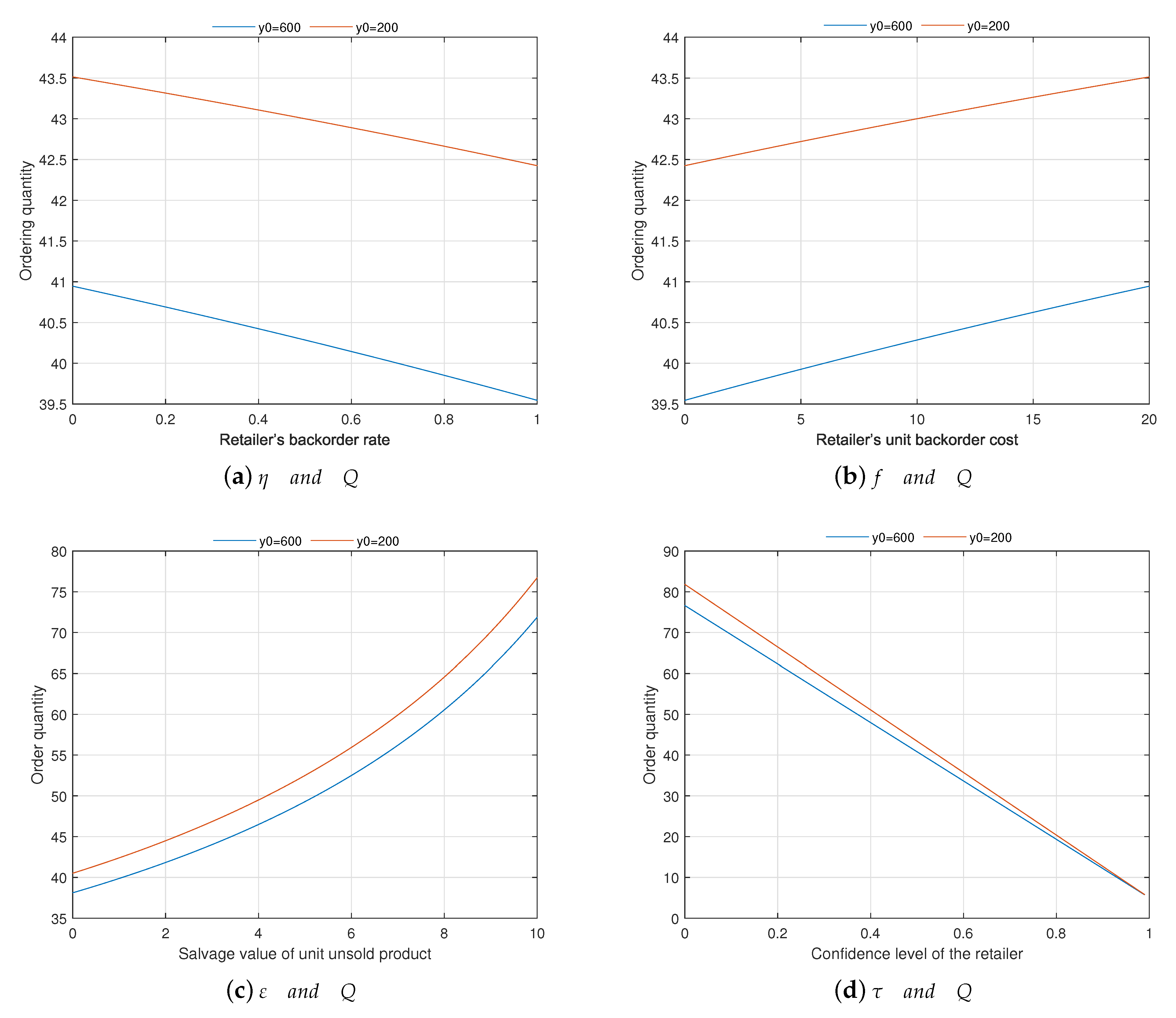
Now, we make sensitivity of the retailer’s parameters by taking $y_0=300,700$ under different financial conditions on the optimal ordering quantity. From Figure 1, we can see that the retailer can make more orders when they adopt a trade credit policy than that uses partial initial capital to make an order. Thus, when the retailer is subjected to the financial constraints, then to motivate the retailer to accept the trade credit strategy rather than the alternative offer from the bank, the supplier would reduce the wholesale price as a way to finally get more profits. From Figure 1a, we can get that when the backorder rate $\eta$ sees a rise, that means more exceeding demands get to be backlogged, the retailer will make a smaller order. From Figure 1b,c, we can see that when the retailer’s unit backorder cost f increases, there will be a higher backorder cost; when the retailer’s residual value of unit unsold goods $\epsilon$ increases, the retailer will have a larger recycling revenue. From this, if he wants to reduce the backorder cost and raise the recycling revenue, the retailer will make a larger order. From Figure 1d, it can be seen that the optimum ordering number Q is falling w.r.t. the confidence level $\tau$. In order to avoid this risk caused by over-ordering, the risk-averse retailer should reduce their order quantity.

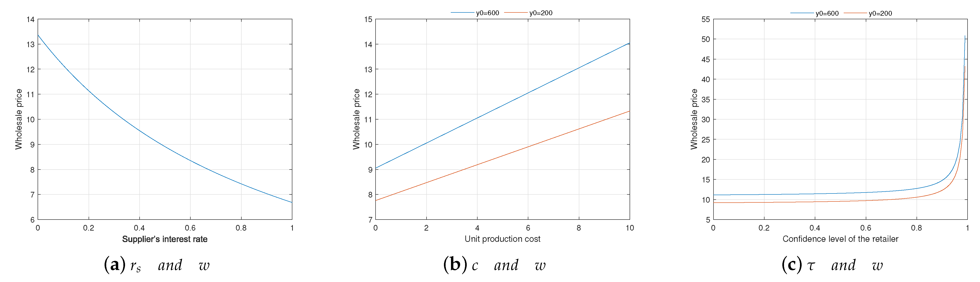
In the following, we make a sensitivity of the retailer’s some parameters under different financial conditions on the optimal wholesale price set by the supplying agent. From Figure 2a, it can be seen that when the retailer is subjected to financial constraints, the supplier tends to lower the wholesale price to motivate the adoption of the trade credit strategy by the retailer rather than the alternative one from the bank. From Figure 2b, we can see a rise in the optimal wholesale price with the suppliers unit production cost c. To avoid the loss brought by excessive production costs, the risk-averse retailer should increase their wholesale price. From Figure 2c, we can see that the confidence level $\tau$ rises meaning a smaller order from the retailer to not fall into the risk of over-ordering. When the retailer orders less, the optimum wholesale price w for a supplier based on the principle of profit maximization will increase with the confidence level $\tau$.

5. Conclusions

This paper investigates the optimal strategy for supply chain with trade credit and backorder under CVaR criterion. For this scenario, the models are established on the purpose of maximizing both the supplier’s and the retailer’s profits, respectively. Based on analyzing the two parties’ benefits in different wealthy regions, both parties’ optimal decisions and how the trade credit is changing the retailer’s mind are obtained. The impact analysis of the backorder and CVaR criterion on the decision variables is also analyzed. It is proved that the increase of the confidence level makes the retailer have to order less to not fall into the risk of over-ordering. When the retailer makes a smaller order, the supplier tends to raise the wholesale price based on the principle of profit maximization. At the same time, this paper finds that backorder will reduce the order numbers of the retailer. Other conclusions are shown as follows: When the retailer uses the trade credit policy, the interest expense (income) of the retailer (supplier) decreases with the initial capital increase, so the retailer (supplier)’s benefit also increases (decreases). When the retailer deposits the remaining funds for ordering goods in the bank to obtain risk-free interest, its interest income increases with the initial capital, so the profit also increases. At the same time, the supplier only received fixed payments for goods and fixed interest income, so the initial funds initially held by the retailer will not affect the supplier’s income. Finally, the proposed model is indicated by the given numerical experiments.

By using the mathematical foundation, our research is quite universal and basically applicable to other enterprises with a two-echelon supply chain. In that sense, this research enriches the trade credit strategy, backorder and CVaR criterion literature in a broader context. However, some limitations leave room for future research. Firstly, we consider the situation in which the capital-constrained retailer adopts the trade credit strategy. In fact, the capital-constrained retailer can also use other financing methods to alleviate financial pressure. Secondly, this paper may not apply to comprehensive enterprises responsible for both production and sales, e.g., agribusiness. Some extensions of the research are as follows. One possible extension is to consider the supplier faces capital constraints. Another possible extension is to incorporate supply chain contracts into this research, which might produce more interesting findings.