The Impacts of Temporary and Permanent Public Health Policies on HRQOL in a Small Open Economy

Abstract

Considering that people can invest in their health-related quality of life (HRQOL), we investigate the effects of public health policies (i.e., a health investment subsidy policy and the direct distribution of health-related goods) on HRQOL in a small open economy. We find that when the government makes public investment in HRQOL temporarily, HRQOL deteriorates or does not improve at least. On the contrary, when public investment is enforced permanently, it improves in the long run.

1. Introduction

The fact that poverty is a major cause of poor health often leads to the presumption that many people in poor countries suffer from ill health because they cannot afford to purchase the items needed for good health, including sufficient quantities of quality food and healthcare. However, being wealthy cannot always solve the problem of poor health. For instance, Kerala, which has an annual per capita income of $1254, has a low rate of infant mortality rate (3.1%); however, Punjab has a rate of infant mortality over 40% even though its income level is twice that of Kerala [1]. Furthermore, Ceara, one of the poorest states in Brazil, has reduced infant mortality by 36% and its rate is now below average in Brazil. Hence, poor countries cannot simply solve the problem of the poor health of their citizens by being wealthy. Furthermore, importantly, poverty is not only a cause of poor health but also a consequence. Infectious and neglected tropical diseases (e.g., HIV, tuberculosis, and malaria) kill and weaken millions of the poorest and most vulnerable people each year. This can seriously reduce economic growth in poor countries as a result of ill health.

Since poverty and poor health are inextricably and causally linked, people in poor countries cannot address this problem easily and thus government intervention plays a pivotal role in resolving the issue. Two facts are important here. First, when discussing government spending including health expenditure, we must recognize the governance issues specific to poor countries, including such topics as democratization, corruption control, capacity-building, and electoral and judicial systems [2]. Although many studies in [2,3,4,5,6,7] argue for the importance of sustained public health programs and systems, the rise in government spending in many poor countries can slow or be repealed. Indeed, by using a panel dataset for 111 countries from 1984 to 2004, the share of GDP devoted to government expenditure in developed countries such as the United States has been steady and increasing since 1970, while government expenditure in developing countries over the past three decades has shown an inconsistent trend [8]. In poor countries, this trend can be generally seen across many kinds of public policies [9,10]. Hence, when we investigate the effects of government expenditure in poor countries, we need to focus on the public policies conducted in a certain period.

Second, turning our interests to health-related public expenditure, some studies have found that such health policies do not create the desirable improvement in health in poor countries. For instance, in poor countries, increasing public spending on health does not lead to lower child mortality [11]. The limited impacts of public spending for the poor at the micro-level, and their findings remain consistent with the small and insignificant impacts of its spending on aggregate health status [12,13]. Health-related public spending in many poor countries does not affect health, with a coefficient that is not statistically significant at conventional levels [1,14]. Similarly, the World Development Report in [15] mentions that no relationship between public expenditure on health and the state of health can be seen at a statistically significant level.

Based on the abovementioned two facts, it can be considered that if the health expenditure of governments is conducted unsteadily (i.e., the temporary enforcement of public policies), it may be difficult for governments in poor countries to resolve the problem of poor health. Then, why does short-term health-related public spending lead to undesirable effects in poor countries? To tackle this problem, we focus on two public policies in the health sector: a price reduction of health-related goods and the direct distribution of such goods. When including these two health policies, we construct a dynamic general equilibrium model of a small open economy with a health status variable.

The health status variable in this study has the following three characteristics. First, it is supposed to represent the health-related quality of life (HRQOL) mentioned by [16,17,18,19]. In [20,21], HRQOL is defined as general perceptions of life satisfaction and quality with respect to health status. Since this is an individual’s physical and mental health over time, the health status variable should be given by the state variable. Furthermore, we assume that when the level of HRQOL increases, an individual’s utility level increases as well. This formations of utility function is fundamentally the same as that in an seminal work of [22], which mentions that it (health) directly enters their preference function, or, put differently, sick days are a source of disutility. As for the validity of the formation of a utility function with a health status variable, when the study in [23] states that by far the most widespread use of this (utility) formulation is with respect to state-dependent variations with individual health status, they estimate the utility functions with the health status variable and assess individuals’ utility functions for health conditions. In addition, by using utility functions with good and poor health, the existing manuscripts [24,25,26] analyze healthcare and health insurance decisions. Therefore, we use the frequently used formation of the utility function with the health status variable.

Second, the health status variable, represented by HRQOL, has evolved over time. Specifically, the level of HRQOL is affected by two elements: health-oriented products and working. When the consumption of health-oriented products such as high-quality food and drink is higher, we assume that the level of HRQOL increases.

Alternatively, we suppose that more working harms the state of health and hence reduces the level of HRQOL. Inhumane working conditions can still be found in poor countries and these often involve inadequate rest, repetitive tasks, exhaustion caused by heavy physical work, a hostile environment or strenuous postures, fatigue, and premature aging caused by a fast work pace and the need for intense vigilance. These factors all harm a worker’s health under long and poorly scheduled working hours. Occupational diseases due to silica or asbestos dust exposure as well as the intake of lead, mercury, and solvents are still widespread in developing countries. There is ample evidence that worker quality dramatically falls without immunization coverage and the outreach of primary care [27].

Similarly, the study in [28] investigates the psychosocial and physical work factors and HRQOL among Iranian industrial workers from steel and cosmetic factories, finding that respondents generally have poor HRQOL. Moreover, the hierarchical regression results for all participants show that work schedule is a significant predictor of all domains of HRQOL.

In this setting, we theoretically find that when a price reduction of health-related goods and the direct distribution of such goods are temporarily enforced, HRQOL deteriorates or does not improve in the long run. To support our findings, we use a numerical simulation and confirm the effectiveness of policy implementation.

Our study is closely related to existing investigations that adopt dynamic macroeconomic models (e.g., [29,30,31,32,33,34]). First, the specification of the utility function with a health status variable is similar to the wealth- or status-seeking preference in [29,30,31] in the sense that the utility function depends on a stock variable. The utility function in their papers depends on the capital stock as well as consumption, implying that people feel happy as their wealth accumulates. On the contrary, our utility function depends on HRQOL, not the capital stock, meaning that an improvement in HRQOL leads to higher utility.

Next, in a two-period overlapping-generation model, the studies in [32,33] introduce healthcare goods. When people consume such goods, their level of utility increases. Hence, healthcare goods can be regarded as consumption goods. In addition, these authors do not introduce any variables to indicate the state of health. In the present study, we introduce a state variable that represents HRQOL, and suppose that an investment commodity can improve HRQOL.

Finally, this study and the existing ones in [34,35] are similarly motivated by the role of foreign aid. In detail, the study in [34] incorporates elastic labor supply into a small open economy and examine the effects of foreign aid on economic growth. By using a New Keynesian small open economy model, the study in [35] numerically examines the impacts of foreign aid as well as government spending. These works do not deal with health-related policies, however, and their focus is not to examine the impacts of temporary policy.

The rest of this paper is organized as follows. In Section 2, we present the baseline model. Section 3 confirms the existence of the steady state and stability. Section 4 examines the effects of a temporary/permanent change in the price reduction of health-related goods. Section 5 examines the impacts of the direct distribution of such related goods. Section 6.1 analyzes the case in which foreign aid is introduced instead of domestic government policies and Section 6.2 provides numerical examples. Section 7 concludes. Finally, in Appendix E, we assume a more general form of the utility function and show that the theoretical findings do not change.

2. Baseline Model

We consider a small open economy facing a constant world interest rate, r. The population is constant and normalized to unity. We consider a simple neoclassical production function. Denoting the time index by t, we express the aggregate production function that satisfies constant returns to scale with respect to capital and labor as

$$y_t=F({\widehat{k}}_t,l_t)=l_{t}f\left(k_t\right),$$

where $y_t$ is output, ${\widehat{k}}_t$ is capital, $l_t$ is labor, and $k_t\equiv {\widehat{k}}_t/l_t$ denotes capital intensity. The production function, $f\left(k_t\right)$, is monotonically increasing, strictly concave in $k_t$, and satisfies the Inada conditions. Taking account of competitive factors and final goods markets, the real rent $r_t$ and real wage rate $w_t$ are respectively determined by

$$r=f^{\prime }\left(k_t\right),w_t=f\left(k_t\right)-k_t{f}^{\prime }\left(k_t\right).$$

(1)

Since the real rent is constant in the small open economy, from Equation (1) we can see that capital intensity is constant and hence the wage rate is fixed as well ($k_t=k$ and $w_t=w$). As a consequence, the production function is given by

$$y_t=l_{t}f\left(k\right).$$

(2)

2.1. Households and Health

HRQOL is a concept that shows the physical and psychological domains of health status. Considering that HRQOL consists of a feeling of satisfaction and sense of happiness (e.g., see [36]), our assumption is that individuals choose goods and services that enhance their HRQOL within the constraints of the resources they possess. Denoting the level of HRQOL by $h_t(>0)$, we assume that HRQOL is incorporated into individuals’ well-being as follows:

$$\begin{array}{c}\hfill U_0\equiv {\int }_0^{\infty }\left\{u\left(c_t\right)+v\left(h_t\right)\right\}{e}^{-\rho t}dt,\end{array}$$

(3)

where $c_t(>0)$ is the level of consumption at time t, $\rho (>0)$ is the rate of time preference, and $h_t(>0)$ shows the level of HRQOL. We assume that $u^{\prime }(·)>0$, $u^{″}(·)<0$, $v^{\prime }(·)>0$, and $v^{″}(·)<0$. In other words, the utility function $v(·)$ shows a positive mood/satisfaction/happiness evaluating HRQOL. Furthermore, these functions satisfy the following Inada conditions: ${lim}_{c_t\to 0}{u}^{\prime }\left(c_t\right)=0$, ${lim}_{c_t\to \infty }{u}^{\prime }\left(c_t\right)=0$, ${lim}_{h_t\to 0}{v}^{\prime }\left(h_t\right)=\infty$, and ${lim}_{h_t\to \infty }{v}^{\prime }\left(h_t\right)=0$.

We assume that the degree of HRQOL $h_t$ is evolved as follows:

$$\begin{array}{c}\hfill {\dot{h}}_t=g(x_t+\eta )-G\left(l_t\right),\end{array}$$

(4)

where $\eta$ represents the public investment health policy and $x_t$ is private spending on health-related goods. We assume that $g^{\prime }(·)>0$, $g^{″}(·)<0$, $G^{\prime }(·)>0$, and $G^{″}(·)>0$, and these functions satisfy the Inada conditions. The negative relationship between the level of labor supply and that of HRQOL means that a larger labor supply leads to a lower utility level $v(·)$ as a result of a lower level of HRQOL. As for private spending on health-related goods $x_t$, for instance, when more working deteriorates physical health, the variable $x_t$ may be regarded as health-oriented products such as high-quality food and drink. When more working harms mental health, it can be thought to be investment in consumption goods that improve mental health.

Next, $\eta$ represents the direct distribution of health-related goods in the form of perfect substitution. Because citizens in lower-middle income countries cannot cost such health-related goods, this kind of government assistance is widely observed. It can be presumed that a larger amount of the direct distribution of health-related goods improves the level of HRQOL, and furthermore, individuals do not cost these goods largely because of the government assistance. As for $g=g(x_t,\eta )$ with ${\partial }^{2}g/(\partial x_t\partial \eta )>0$, which means that the government assistance corresponds to sanitation and DDT sparying for malaria control, we will mention the effects of public policy later.

Turning our interest to the budget constraint, we suppose that by using the goods produced by the capital stock, the representative agent has the option of either consuming or investing in health. Then, the accumulation of foreign asset holdings, $b_t$ evolves as

$$\begin{array}{c}\hfill {\dot{b}}_t=r{b}_t+l_{t}f\left(k\right)-c_t-(1-\tau )x_t-z_t,\end{array}$$

(5)

where $z_t$ is the lump-sum tax and $\tau$ represents the price reduction of health-related goods. An increase in $\tau$ decreases the relative price of health-related goods and hence stimulate the health-related investment further, leading to a higher level of HRQOL $h_t$.

We assume that the government levies a lump-sum tax on its budget to keep the following balanced budget over time:

$$\begin{array}{c}\hfill \tau x_t+\eta =z_t.\end{array}$$

(6)

2.2. Dynamic System

The representative agent maximizes his or her lifelong utility Equation (3) subject to the evolution of HRQOL Equation (4) and the budget constraint Equation (5). To derive the optimal conditions, we set the current-value Hamiltonian:

$$\begin{array}{cc}\hfill \mathcal{H}=u\left(c_t\right)+v\left(h_t\right)& +{\lambda }_t\left[g(x_t+\eta )-G\left(l_t\right)\right]\hfill \\ \hfill & +q_t\left[r{b}_t+l_{t}f\left(k\right)-c_t-(1-\tau )x_t-z_t\right],\hfill \end{array}$$

where ${\lambda }_t$ and $q_t$ are the costate variables for Equations (4) and (5), respectively.

By deriving the optimal conditions, we have

$$\begin{array}{cc}\hfill u^{\prime }\left(c_t\right)& =q_t,\hfill \end{array}$$

(7a)

$$\begin{array}{cc}\hfill v^{\prime }\left(h_t\right)& =-{\dot{\lambda }}_t+\rho {\lambda }_t,\hfill \end{array}$$

(7b)

$$\begin{array}{cc}\hfill g^{\prime }(x_t+\eta ){\lambda }_t& =(1-\tau )q_t,\hfill \end{array}$$

(7c)

$$\begin{array}{cc}\hfill G^{\prime }\left(l_t\right){\lambda }_t& =q_{t}f\left(k\right),\hfill \end{array}$$

(7d)

$$\begin{array}{cc}\hfill r{q}_t& =-{\dot{q}}_t+\rho q_t.\hfill \end{array}$$

(7e)

The transversality conditions are given by

$$\begin{array}{c}\hfill \underset{t\to \infty }{lim}{\lambda }_t{h}_t{e}^{-\rho t}=0,\underset{t\to \infty }{lim}{q}_t{b}_t{e}^{-\rho t}=0.\end{array}$$

From Equations (7a) and (7e), the well-known Euler equation for consumption is given by

$$\begin{array}{c}\hfill \frac{{\dot{c}}_t}{c_t}=-\frac{u^{\prime }\left(c_t\right)}{c_t{u}^{″}\left(c_t\right)}(r-\rho ).\end{array}$$

(8)

Because of the set-up of the small open economy, which means that the rate of interest is fixed, we have to require $r=\rho$ for our system to have a finite interior steady-state value for the marginal utility of consumption. In sum, since ${\dot{c}}_t=0$ and ${\dot{q}}_t=0$ under $r=\rho$, the level of consumption is constant over time $c_t=\overline{c}$, and the marginal utility of consumption has a finite value $u^{\prime }\left(\overline{c}\right)=q_t=\overline{q}$. Further, the constant level of consumption is endogenously determined as mentioned later.

Next, by using Equation (7c), we obtain

$$\begin{array}{c}\hfill {\lambda }_t=\frac{(1-\tau )u^{\prime }\left(\overline{c}\right)}{g^{\prime }(x_t+\eta )}.\end{array}$$

(9)

By substituting Equations (7b) and (9) into the time derivative of Equation (9), we can see that

$$\begin{array}{c}\hfill {\dot{x}}_t=-\frac{g^{\prime }(x_t+\eta )}{g^{″}(x_t+\eta )}\left\{r-\frac{v^{\prime }\left(h_t\right)g^{\prime }(x_t+\eta )}{(1-\tau )u^{\prime }\left(\overline{c}\right)}\right\}.\end{array}$$

(10)

Equations (7c) and (7d) yield

$$g^{\prime }(x_t+\eta )f\left(k\right)=(1-\tau )G^{\prime }\left(l_t\right).$$

(11)

By totally differentiating Equation (11), we can express $l_t$ as follows:

$$l_t=l(x_t,\tau ,\eta ),$$

(12)

where the signs of the partial derivative are

$$\begin{array}{cc}\hfill l_x\left(\equiv \frac{\partial l_t}{\partial x_t}\right)=l_{\eta }\left(\equiv \frac{\partial l_t}{\partial \eta }\right)& =\frac{g^{″}(x_t+\eta )f\left(k\right)}{(1-\tau )G^{″}\left(l_t\right)}<0,\hfill \end{array}$$

(13a)

$$\begin{array}{cc}\hfill l_{\tau }\left(\equiv \frac{\partial l_t}{\partial \tau }\right)& =\frac{G^{\prime }\left(l_t\right)}{(1-\tau )G^{″}\left(l_t\right)}>0.\hfill \end{array}$$

(13b)

By taking Equations (4) and (12) into consideration, we can rewrite the evolution of HRQOL as follows:

$$\begin{array}{c}\hfill {\dot{h}}_t=g(x_t+\eta )-G\left(l(x_t,\tau ,\eta )\right).\end{array}$$

(14)

From Equations (6) and (12), we can show the accumulation equation of foreign assets (Equation (5)) as follows:

$$\begin{array}{c}\hfill {\dot{b}}_t=r{b}_t+l(x_t,\tau ,\eta )f\left(k\right)-\overline{c}-x_t-\eta .\end{array}$$

(15)

Therefore, the complete dynamic system is provided by Equations (10), (14), and (15) given a constant level of consumption $\overline{c}$, the rate of investment subsidy $\tau$, and the direct transfer of health investment $\eta$ at which the level of $\overline{c}$ is endogenously determined.

3. Steady State and Stability

Supposing that the initial levels of HRQOL and foreign assets are $h_{t_0}$ and $b_{t_0}$, respectively, we now denote the steady-state levels of the variables by the asterisk $\{h_j^{*},x_j^{*},b_j^{*},{\overline{c}}_j^{*}\}$, where the policy instruments are represented by ${\tau }_j$ and ${\eta }_j$. Notice that the subscript j shows just a number that stands for each steady state as in [37]. In the dynamic system (Equations (10) and (14)), we now analyze the existence of the uniquely determined steady state and its stability.

From Equation (10), we show that the ${\dot{x}}_t=0$ locus is

$$\begin{array}{c}\hfill g^{\prime }(x_j^{*}+{\eta }_j)=\frac{r(1-{\tau }_j)u^{\prime }\left({\overline{c}}_j^{*}\right)}{v^{\prime }\left(h_j^{*}\right)},\end{array}$$

(16a)

where the slope of the ${\dot{x}}_t=0$ locus is given by

$$\begin{array}{c}\hfill \frac{d{x}_t}{d{h}_t}{|}_{{\dot{x}}_t=0}=-\frac{g^{\prime }(x_j^{*}+{\eta }_j)}{g^{″}(x_j^{*}+{\eta }_j)}\frac{v^{″}\left(h_j^{*}\right)}{v^{\prime }\left(h_j^{*}\right)}<0.\end{array}$$

(16b)

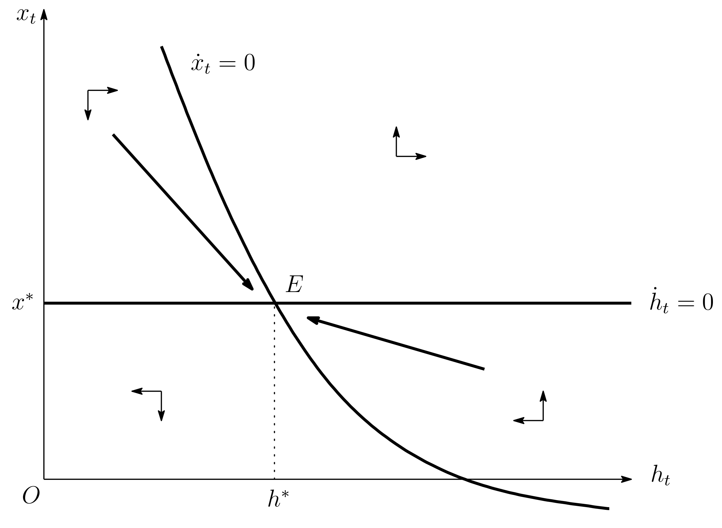
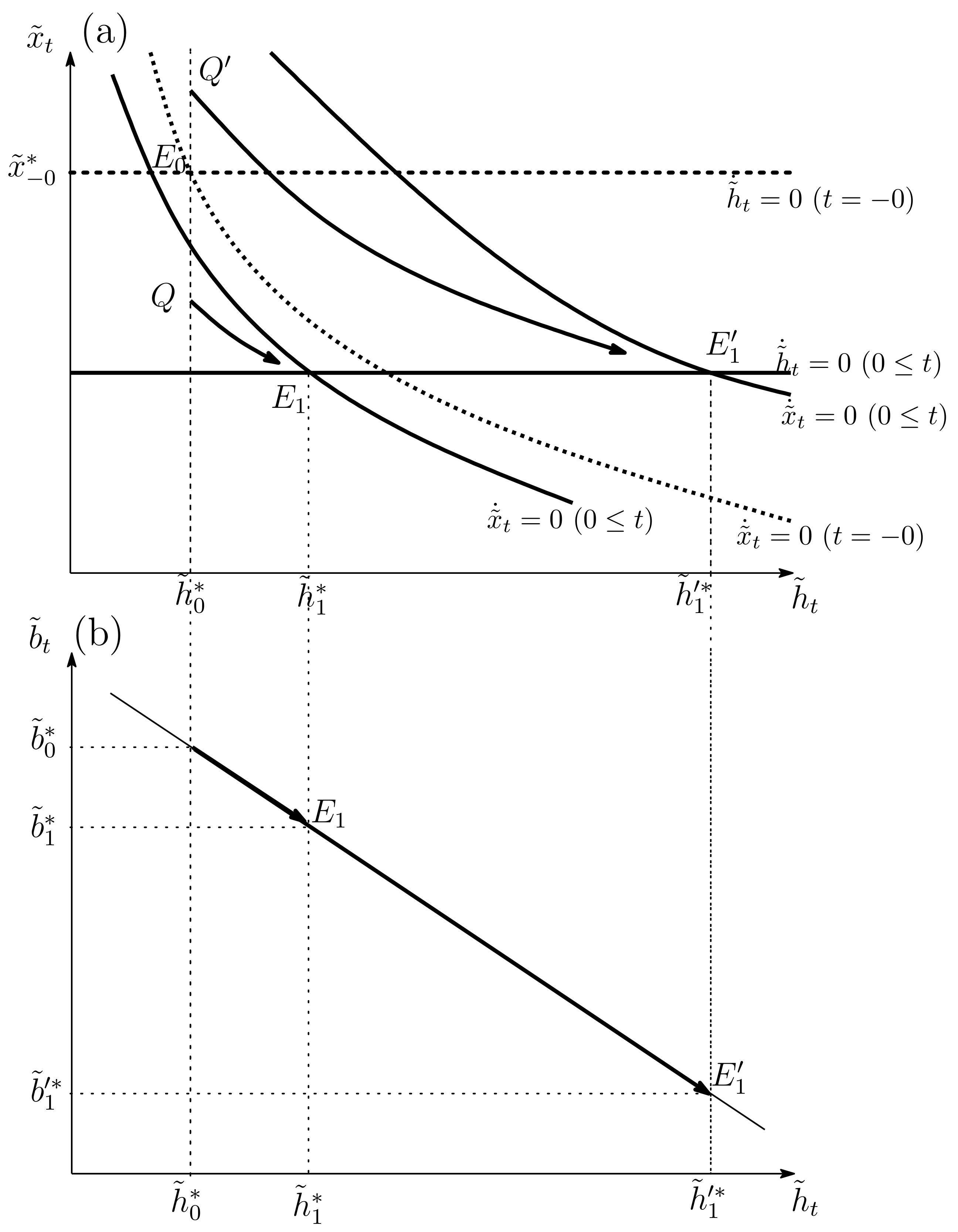
The level of $x_j^{*}$ approaches infinity as the level of $h_j^{*}$ goes to zero, while it approaches a negative value $-\eta$ as the level of HRQOL goes to infinity. Then, the ${\dot{x}}_t=0$ locus can be depicted by the lower right curve in Figure 1.

Turning to the equation ${\dot{h}}_t=0$, from Equation (14), we can see that

$$g(x_j^{*}+{\eta }_j)=G\left(l(x_j^{*},{\tau }_j,{\eta }_j)\right).$$

(17)

Noting that ${\dot{h}}_t=0$ is a horizontal line as in Figure 1, we can confirm that the level of $x_j^{*}$ is uniquely determined. As a result, we can easily see that there exists a unique steady state given a fixed level of private consumption. More concretely, from Equations (10) and (14), the dynamics of $x_t$ and $h_t$ are respectively characterized by $\frac{\partial {\dot{x}}_t}{\partial h_t}{|}_{x_t=\mathrm{const}}=r\frac{g^{\prime }}{g^{″}}\frac{v^{″}}{v^{\prime }}>0$ and $\frac{\partial {\dot{h}}_t}{\partial x_t}{|}_{h_t=\mathrm{const}}=g^{\prime }-G^{\prime }{l}_x>0.$ Thus, we can see that ${\dot{x}}_t>0$ above the ${\dot{x}}_t=0$ locus (${\dot{x}}_t<0$ below the ${\dot{x}}_t=0$ locus) and that ${\dot{h}}_t>0$ above the ${\dot{h}}_t=0$ locus (${\dot{h}}_t<0$ below the ${\dot{h}}_t=0$ locus). Figure 1 illustrates the phase diagram.

To examine the stability of the steady state, from Equations (10) and (14), we obtain the linearly approximated equations:

$$\begin{array}{c}\hfill \left[\begin{array}{c}{\dot{x}}_t\\ {\dot{h}}_t\end{array}\right]=\underset{\equiv J}{\underbrace{\left[\begin{array}{cc}{J}_j^{11}& J_j^{12}\\ J_j^{21}& J_j^{22}\end{array}\right]}}\left[\begin{array}{c}{x}_t-x_j^{*}\\ h_t-h_j^{*}\end{array}\right],\end{array}$$

(18a)

where

$$\begin{array}{c}{J}_j^{11}\equiv \frac{\partial {\dot{x}}_t}{\partial x_t}=\frac{v^{\prime }\left(h_j^{*}\right)g^{\prime }(x_j^{*}+{\eta }_j)}{(1-\tau )u^{\prime }\left({\overline{c}}_j^{*}\right)}=r>0, J_j^{12}\equiv \frac{\partial {\dot{x}}_t}{\partial h_t}=r\frac{g^{\prime }(x_j^{*}+{\eta }_j)}{g^{″}(x_j^{*}+{\eta }_j)}\frac{v^{″}\left(h_j^{*}\right)}{v^{\prime }\left(h_j^{*}\right)}>0, \\ J_j^{21}\equiv \frac{\partial {\dot{h}}_t}{\partial x_t}=g^{\prime }(x_j^{*}+{\eta }_j)-G^{\prime }\left(l_j^{*}\right)l_x>0, J_j^{22}\equiv \frac{\partial {\dot{h}}_t}{\partial h_t}=0.\end{array}$$

Concerning the coefficient matrix of Equation (18a), we can see that

$$\mathrm{Tr}J=r>0,\mathrm{Det}J=-r\frac{g^{\prime }(x_j^{*}+{\eta }_j)}{g^{″}(x_j^{*}+{\eta }_j)}\frac{v^{″}\left(h_j^{*}\right)}{v^{\prime }\left(h_j^{*}\right)}\left\{g^{\prime }(x_j^{*}+{\eta }_j)-G^{\prime }\left(l_j^{*}\right)l_x\right\}<0.$$

(18b)

Hence, our model has saddle-path stability because the two eigenvalues of the coefficient matrix have opposite signs. The stable and unstable roots are given by

$$\begin{array}{c}\hfill a_j^s=\frac{1}{2}\left(r-\sqrt{r^2+4J_j^{12}{J}_j^{21}}\right)<0,a_j^u=\frac{1}{2}\left(r+\sqrt{r^2+4J_j^{12}{J}_j^{21}}\right)>0.\end{array}$$

(19)

Then, we obtain the following proposition.

Proposition 1.

The steady-state equilibrium is uniquely determined and satisfies saddle-path stability given the fixed level of private consumption.

Based on Proposition 1, from ${\dot{b}}_t=0$ equation we can find that the steady-state level of foreign assets is also determined given the fixed level of private consumption:

$$r{b}_j^{*}+l(x_j^{*},{\tau }_j,{\eta }_j)f\left(k\right)-{\overline{c}}_j^{*}-x_j^{*}-{\eta }_j=0.$$

(20)

Finally, by using the linear approximation of $(h_t,x_t,b_t)$, we can determine the level of private consumption as in [37,38]:

$$\begin{array}{cc}\hfill h_t& =h_j^{*}+A_j^s{e}^{a_j^{s}t}+A_j^u{e}^{a_j^{u}t},\hfill \end{array}$$

(21a)

$$\begin{array}{cc}\hfill x_t& =x_j^{*}+{\Theta }_j^s{A}_j^s{e}^{a_j^{s}t}+{\Theta }_j^u{A}_j^u{e}^{a_j^{u}t},\hfill \end{array}$$

(21b)

where

$${\Theta }_j^s\equiv \frac{a_j^s-r}{J_j^{12}}<0,{\Theta }_j^u\equiv \frac{a_j^u-r}{J_j^{12}}>0.$$

(21c)

Note that $a_j^u-r=\frac{1}{2}\left(-r+\sqrt{r^2+4J_j^{12}{J}_j^{21}}\right)(>0)$, where $J_j^{12}{J}_j^{21}>0$.

To derive the linear approximation of the foreign asset, we use Equation (15) as follows:

$$\begin{array}{c}\hfill {\dot{b}}_t={\Omega }_j(x_t-x_j^{*})+r(b_t-b_j^{*}),{\Omega }_j\equiv f\left(k\right)l_{x,j}-1<0.\end{array}$$

(22)

By solving Equation (22), we have

$$\begin{array}{c}\hfill b_t=b_j^{*}+\frac{{\Omega }_j\left(A_j^s{e}^{a_j^{s}t}+A_j^u{e}^{a_j^{u}t}\right)}{J_j^{12}}+S{e}^{rt},\end{array}$$

(23)

where we use ${\Theta }_j/(a_j^n-r)=\frac{1}{J_j^{12}}$$(n=s,u)$. The variable S is as follows:

$$S\equiv b_{t_0}-b_j^{*}-\frac{{\Omega }_j}{J_j^{12}}\left(A_j^s{e}^{a_j^s{t}_0}+A_j^u{e}^{a_j^u{t}_0}\right),$$

(24)

where $t_0$ is the initial period.

When $S\ne 0$, the economy monotonically expands over time irrespective of the values of $a_j^s$, $a_j^u$, $A_j^s$, and $A_j^u$. Therefore, we assume the solvency condition (i.e., $S=0$) in Equation (24). In particular, by setting $t=t_0$ in Equation (21a), we can obtain $A_j^s{e}^{a_j^s{t}_0}+A_j^u{e}^{a_j^u{t}_0}=h_{t_0}-h_j^{*}$. By substituting this equation into Equation (24), we can obtain

$$b_{t_0}-b_j^{*}=\frac{{\Omega }_j}{J_j^{12}}\left(h_{t_0}-h_j^{*}\right).$$

(25)

The level of $x_j^{*}$ is determined by only Equation (17), which means that the steady-state level of public spending on health-related goods does not depend on the constant level of private consumption. After the determination of the level of $x_j^{*}$, Equations (16a), (20), and (25) determine the steady-state levels of HRQOL and foreign assets as well as the constant level of private consumption.

4. Price Reduction of Health-Related Goods

We consider the case in which the government announces a change in the policy instruments from the original level, ${\tau }_0$, to a new level, ${\tau }_1$, at time $t=t_0=0$ (hereafter, we just say $t=0$); the policy is conducted permanently or temporarily. Then, we can see that after the initial consumption jumps due to the policy change, the level of consumption becomes fixed because the growth rate of consumption is zero under the assumption that $r=\rho$. In particular, we must note the case of the temporary enforcement of the health policy, as even if the policy instrument returns to the original level at time T, the level of consumption does not change, and therefore, the level of consumption does not go back to its original level under the assumption of perfect foresight. This is because agents can initially anticipate the policy change at time T.

4.1. Permanent Price Reduction

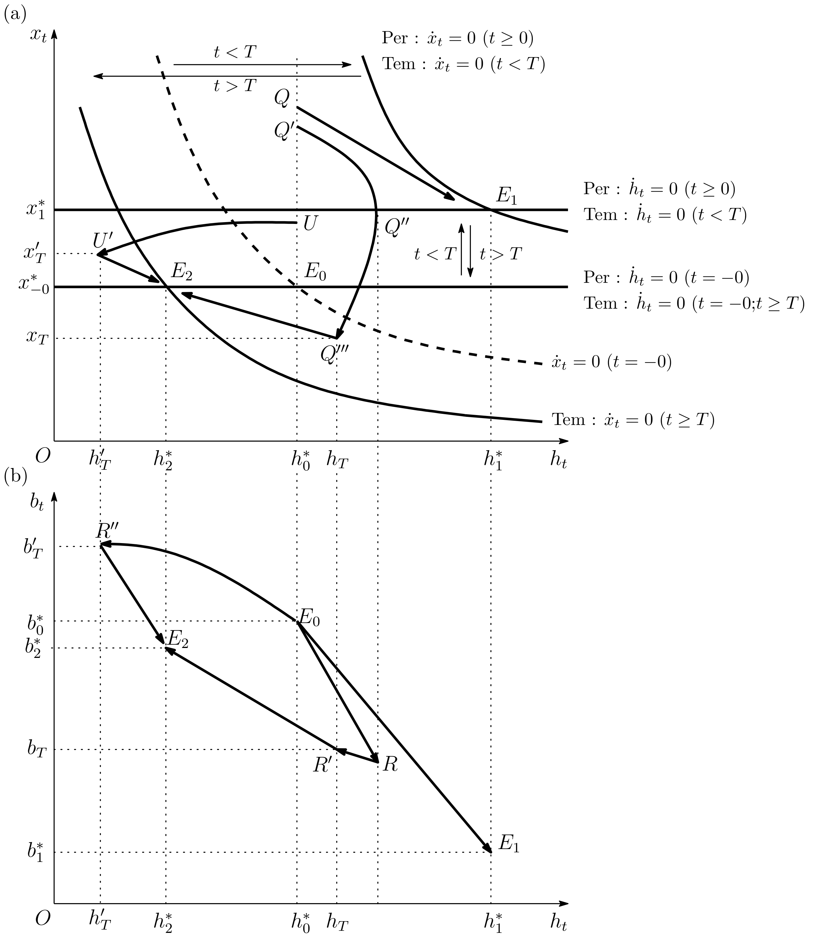
Suppose that the price reduction is implemented permanently (i.e., a permanent increase in $\tau$). Then, we can see that the shift in the ${\dot{x}}_t=0$ locus is as follows:

$$\begin{array}{cc}\hfill \frac{\partial x_t}{\partial \tau }{|}_{{\dot{x}}_t=0,h^{*}=\mathrm{constant}}& =\underset{(+)}{\underbrace{-\frac{(1-\tau )r{u}^{\prime }\left(\overline{c}\right)}{v^{\prime }\left(h_t\right)g^{″}\left(x_t\right)}}}\left(\underset{(\#1)}{\underbrace{\frac{1}{1-\tau }}}\underset{(\#2)}{\underbrace{-\frac{u^{″}\left(\overline{c}\right)}{u^{\prime }\left(\overline{c}\right)}{C}_{\tau }}}\right)>0,\hfill \end{array}$$

(26a)

where $C_{\tau }(<0)$ shows the impact of the policy change in $\tau$ on consumption. See Appendix A for the sign of Equation (26a) and Appendix B for the negative sign of $C_{\tau }$. The term $(\#1)$ has a positive sign, while the term $(\#2)$ has a negative one. Although the two terms have the opposite sign, the direct impact in $(\#1)$ always dominates the indirect one in the term $(\#2)$, resulting in an upward shift in the ${\dot{x}}_t=0$ locus as depicted in Figure 2a. Next, we can see the shift in the ${\dot{h}}_t=0$ locus as follows:

$$\begin{array}{cc}\hfill \frac{\partial x_t}{\partial \tau }& =\frac{G^{\prime }\left(l_t\right)l_{\tau }}{g^{\prime }\left(x_t\right)-G^{\prime }\left(l_t\right)l_x}>0.\hfill \end{array}$$

(26b)

An increase in $\tau$ yields an upward shift in the ${\dot{h}}_t=0$ locus.

Assuming that the policy is enforced at time 0, we denote the levels of the variables at the original steady state by $\{h_0^{*},x_{-0}^{*},b_0^{*},{\overline{c}}_{-0}^{*}\}$ before $t_0=0$. Since the control variables of x and $\overline{c}$ jump at time 0, we must note that the levels of these control variables are not the same as the original steady-state levels (that is, $x_0\ne x_{-0}^{*}$ and ${\overline{c}}_0\ne {\overline{c}}_{-0}^{*}$), and that the levels of state variables h and b at time 0 are the same as the original steady-state levels (that is, $h_{-0}^{*}=h_0^{*}$ and $b_{-0}^{*}=b_0^{*}$).

By denoting the levels of the variables at the new steady state by $\{h_1^{*},x_1^{*},b_1^{*},{\overline{c}}_1^{*}\}$, we obtain the following proposition.

Proposition 2.

A permanent price reduction of health-related goods (i.e., a permanent increase in τ) leads to $h_0^{*}<h_1^{*}$, $x_{-0}^{*}<x_1^{*}<x_0$, ${\overline{c}}_{-0}^{*}>{\overline{c}}_1^{*}={\overline{c}}_0^{*}$, and $b_0^{*}>b_1^{*}$.

Proof. 

Taking account of Equations (26a) and (26b), from Figure 2a we can confirm that $h_0^{*}<h_1^{*}$ and $x_{-0}^{*}<x_1^{*}$. As for private consumption, after its initial jump, its level is constant over time. In other words, it holds that ${\overline{c}}_0^{*}={\overline{c}}_1^{*}$. Appendix B shows that ${\overline{c}}_{-0}^{*}>{\overline{c}}_0^{*}$ and $x_1^{*}<x_0$. □

Now, we confirm the impact of a permanent rise in $\tau$ in Figure 2. Suppose that the economy is initially in the original steady state $E_0$ as in Figure 2a and that the government raises $\tau$ permanently at time $t=0$. Then, the ${\dot{x}}_t=0$ locus moves upwardly from “${\dot{x}}_t=0$ ($t=-0$)” to “Per: ${\dot{x}}_t=0$ ($t\ge 0$).” Furthermore, since the ${\dot{h}}_t=0$ locus also shifts upward under a permanent rise in $\tau$, the graph of the ${\dot{h}}_t=0$ locus moves from “${\dot{h}}_t=0$ ($t=-0$)” to “Per: ${\dot{h}}_t=0$ ($t\ge 0$).” In this case, spending on health-related goods, $x_t$, first jumps to “Q” to ride on the new saddle path ($x_0>x_1^{*}$); thereafter, the level of $x_t$ decreases towards the new steady state. However, it holds that $x_1^{*}>x_{-0}^{*}$. On the contrary, the level of HRQOL continues to improve along this saddle path, showing that its level in the new steady state $E_1$ is greater than the original level. Figure 2b depicts the relationship between $h_t$ and $b_t$. Under a permanent rise in $\tau$, the steady-state value of $b_t$ ends up decreasing to satisfy the solvency condition.

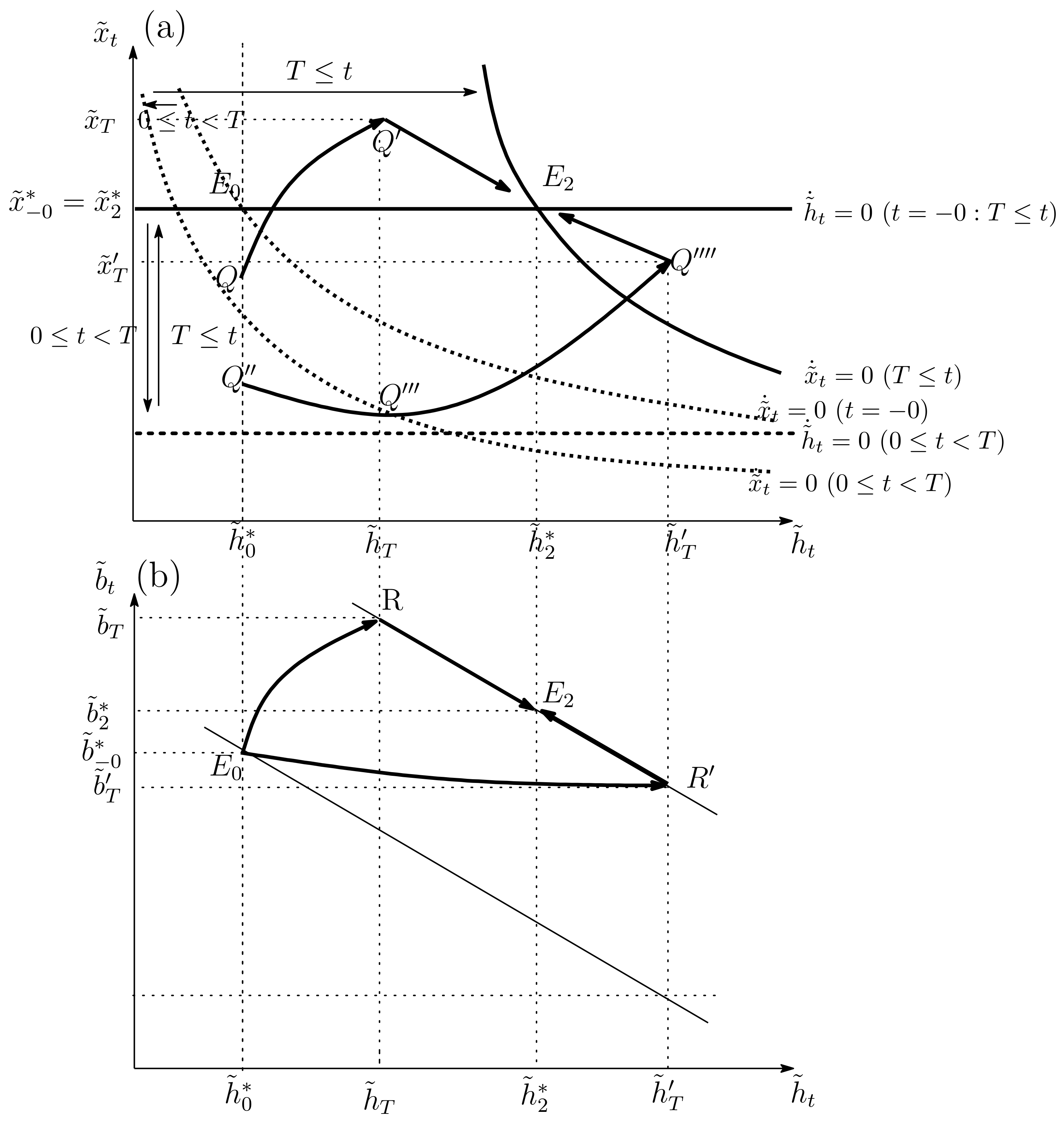
4.2. Temporary Price Reduction

We now suppose that the government makes the price reduction of health-related goods during some duration $t=[0,T)$ and then the policy instruments permanently return to the original level ${\tau }_0$ during $t=[T,\infty ]$. As denoted in the last subsection, the original steady state before $t=0$ (the period of the policy change) is characterized by $\{h_0^{*},x_{-0}^{*},b_0^{*},{\overline{c}}_{-0}^{*}\}$ and the new steady state is given by $\{h_2^{*},x_2^{*},b_2^{*},{\overline{c}}_2^{*}\}$ after the health policy is returned at time T. Then, we can analytically prove the following.

Proposition 3.

A temporary price reduction of health-related goods (i.e., a temporary increase in τ) leads to $h_0^{*}>h_2^{*}$, $x_{-0}^{*}=x_2^{*}$, ${\overline{c}}_{-0}^{*}>{\overline{c}}_2^{*}={\overline{c}}_0^{*}$, and $b_0^{*}>b_2^{*}$.

Proof. 

Since the steady-state level of health-related goods does not depend on the levels of private consumption, it holds that the new steady-state level of health-related goods and its original one are the same (i.e., $x_{-0}^{*}=x_2^{*}$). See Equation (17) under $\tau ={\tau }_0$. Therefore, it also holds that $l_{-0}^{*}=l_2^{*}$. We prove that the initial jump in private consumption is downward (that is, ${\overline{c}}_{-0}^{*}>{\overline{c}}_2^{*}={\overline{c}}_0^{*}$) in Appendix B. The level of consumption stays at the new steady state at time 0. In addition, we show that $h_0^{*}>h_2^{*}$ in Appendix C. Finally, taking account of ${\overline{c}}_{-0}^{*}>{\overline{c}}_2^{*}$, $l_{-0}^{*}=l_2^{*}$ and $x_{-0}^{*}=x_2^{*}$, from Equation (20), we find that $b_0^{*}>b_2^{*}$. □

A temporary price reduction of health-related goods leads to a negative impact on consumption at time 0 because the policy decreases the relative price of health-related goods and hence causes further investment in HRQOL. Therefore, the direction of the initial jump in consumption is downward. After this health policy is removed, the level of private consumption does not return to the original level and continues to stay at the new level to maintain the solvency condition in Equation (24). As a result, the lower level of private consumption negatively affects the growth rate of spending on health-related goods in Equation (10) over time. Put differently, current health investment is substituted for future investment, which delays health investment. Considering that only the negative impact on consumption remains in the long run after the health policy is removed, we can show that the long-run effect that affects HRQOL consists of only the delay in health investment; hence, the temporary price reduction of health-related goods lowers the long-run level of HRQOL. Alternatively, since the steady-state level of health-related goods does not depend on the level of private consumption in Equation (17), the level of health-related goods returns to its original level ($x_{-0}^{*}=x_2^{*}$). In other words, although the level of health-related goods before the policy is the same as that in the new steady state, HRQOL is deteriorated in the new steady state because of the downward jump in consumption. Finally, the lower level of consumption in the long run means a lower level of the shadow value of future consumption (the accumulation of foreign assets) $\overline{q}$. Since households do not have a strong motivation to save, the level of foreign assets in the long run is lower than its original level.

Figure 2 shows the dynamic movement of the economy, highlighting that the original steady state is given by $E_0$ before the policy enforcement. When the government raises $\tau$ from ${\tau }_0$ to ${\tau }_1$ at time $t=0$ and restores ${\tau }_1$ to ${\tau }_0$ after $t=T$, the graph of the ${\dot{x}}_t=0$ locus first shifts upward (from “${\dot{x}}_t=0$ ($t=-0$)” to “Tem: ${\dot{x}}_t=0$ ($t<T$)” in Figure 2a) and then moves downward (from “Tem: ${\dot{x}}_t=0$ ($t<T$)” to “Tem: ${\dot{x}}_t=0$ ($t>T$)”). Regarding the ${\dot{h}}_t=0$ locus, the graph first shifts upward (from “${\dot{h}}_t=0$ ($t=-0;t\ge T$)” to “Tem: ${\dot{h}}_t=0$ ($t<T$)”) and then moves downward (from “Tem: ${\dot{h}}_t=0$ ($t<T$)” to “Tem: ${\dot{h}}_t=0$ ($t=0;t\ge T$)”). Suppose that the level of $x_t$ initially jumps to point $Q^{\prime }$, which is greater than the level of $x_1^{*}$. Then, the economy moves along an unstable path through point $Q^{″}$ towards point $Q^{″\prime }$. After the temporary price reduction of health-related goods is removed at time $t=T$, the economy rides on the new saddle path. Therefore, the level of HRQOL decreases monotonically and is ultimately lower than its initial level. Figure 2b shows the relationship between $h_t$ and $b_t$. Under a temporary rise in $\tau$, the level of foreign assets decreases from $E_0$ to R and then increases until the new steady state $E_2$; however, the level of foreign assets at the steady state $E_2$ is lower than the level at the original steady state $E_0$.

In what follows, we consider the case in which the upward jump in spending on health-related goods is not so large from the original steady state $E_0$ to point U. After the initial jump, the levels of both HRQOL and spending on health-related goods decrease during the enforcement of the price reduction. After the removal of the price reduction policy, the economy arrives at point $U^{\prime }$. Thereafter, the level of HRQOL increases during time $t\in [T,\infty ]$. In this case, the level of foreign assets increases for $t\in [0,T)$ and then decreases after the removal of the health policy.

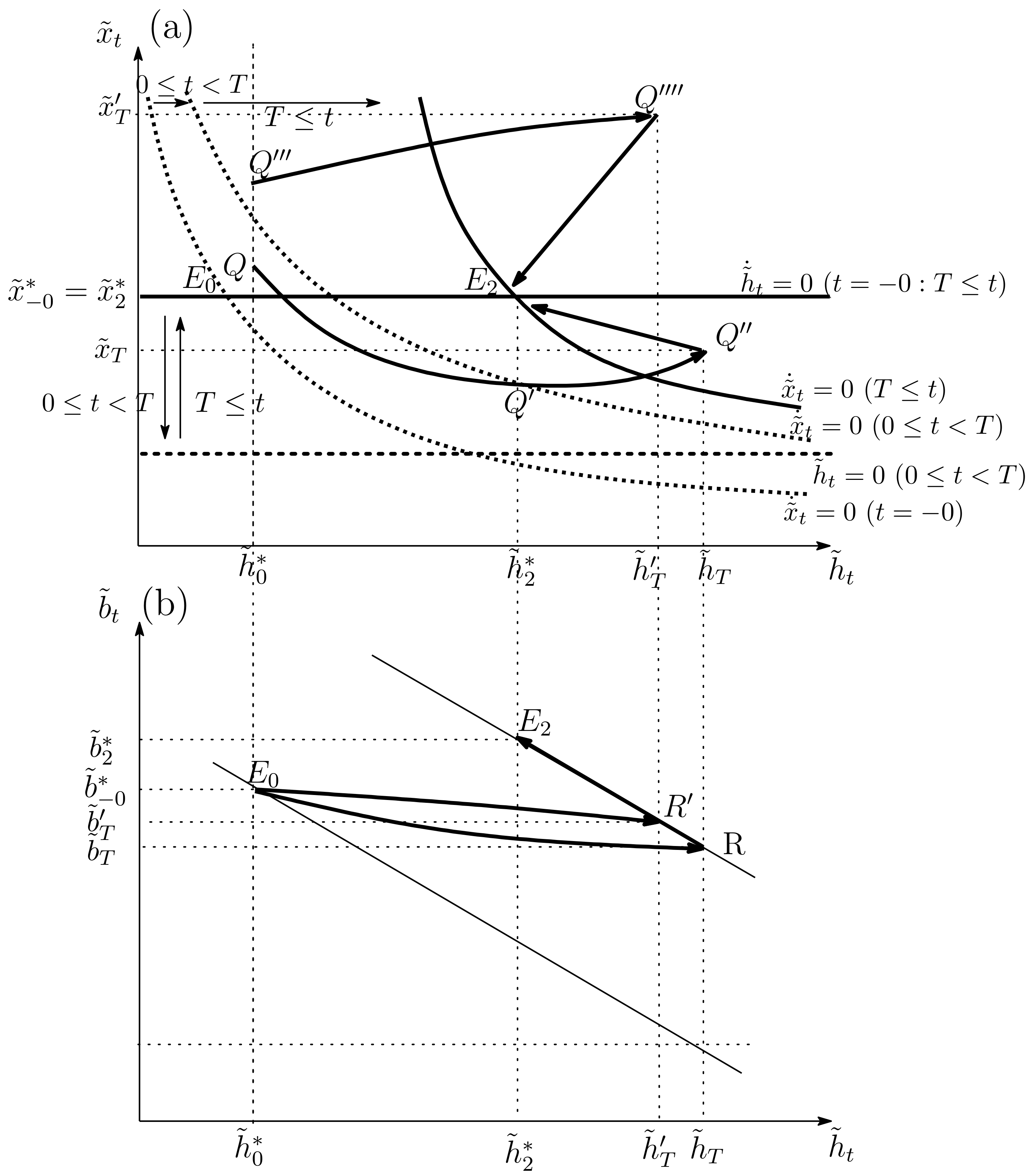
5. Direct Distribution of Health-Related Goods

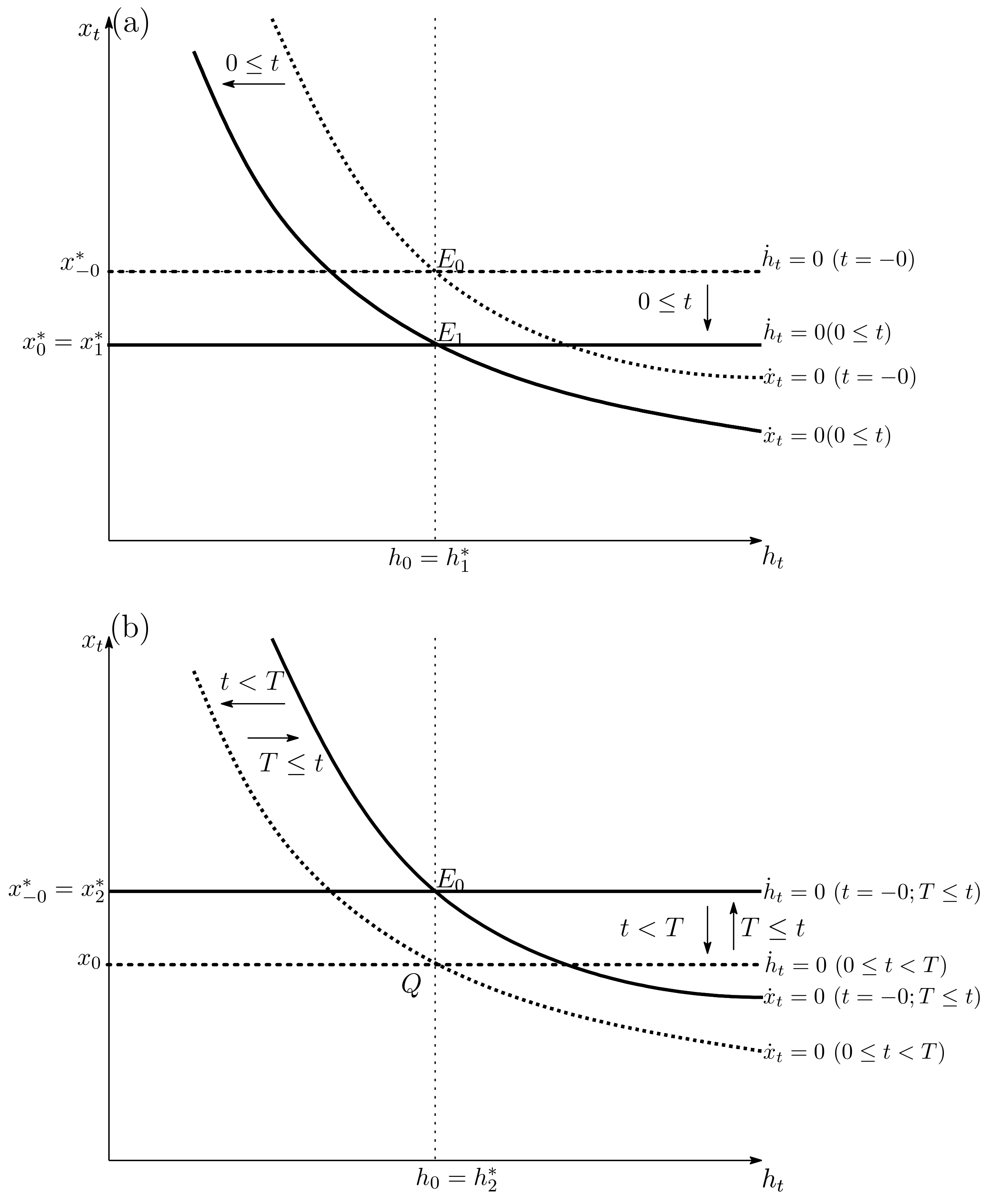
In this section, we consider the effects of the direct distribution of health-related goods (i.e., an increase in $\eta$). From Equation (17), we can see that $\frac{\partial x^{*}}{\partial \eta }=-1$ because $l_x=l_{\eta }$ in Equation (13a). In other words, since the relationship between health-related goods $x_t$ and the transfer $\eta$ is completely substitutable, a one-unit increase in the direct distribution of health-related goods causes a one-unit decrease in health-related goods. Therefore, public investment in HRQOL crowds out private spending on health-related goods. As shown in Figure 3a,b, the crowding out effect for health-related goods leads to downward shifts in the $\dot{x}=0$ and $\dot{h}=0$ loci:

$$\frac{\partial x}{\partial \eta }{|}_{\dot{x}=0,h^{*}=\mathrm{const}}=\frac{\partial x}{\partial \eta }{|}_{\dot{h}=0,h^{*}=\mathrm{const}}=-1.$$

(27)

Figure 3a shows that the permanent increase in $\eta$ alone makes spending on health-related goods decrease because the perfect substitution between health-related goods and the health policy does not change HRQOL. Alternatively, since the level of HRQOL does not move, the level of foreign assets does not move. We omit the dynamic motion of foreign assets because the dynamic behavior is trivial.

When the distribution of health-related goods is enforced temporarily, Figure 3b shows that the level of $x_2^{*}$ is the same as its original level $x_{-0}^{*}$. The crowding out effect does not affect private consumption. In addition, Appendix D shows the theoretical investigations. In sum, it holds that ${\overline{c}}_{-0}^{*}={\overline{c}}_t$ over time. Hence, a temporary increase in $\eta$ does not cause any changes in the long run as seen in Figure 3b.

Figure 3 illustrates that the crowding out effect of public investment in HRQOL gives insignificant results in this economy. In that regard, some researchers similarly argue that the crowding out effect makes government spending on health negligible [11,39,40,41]. For instance, the study in [40] writes, “Why does public expenditure on average have such a limited effect on health (and education) outcomes? … A large portion of public spending on health (and education) is devoted to private goods—ones where government spending is likely to crowd out private spending.” This is just the case that we show.

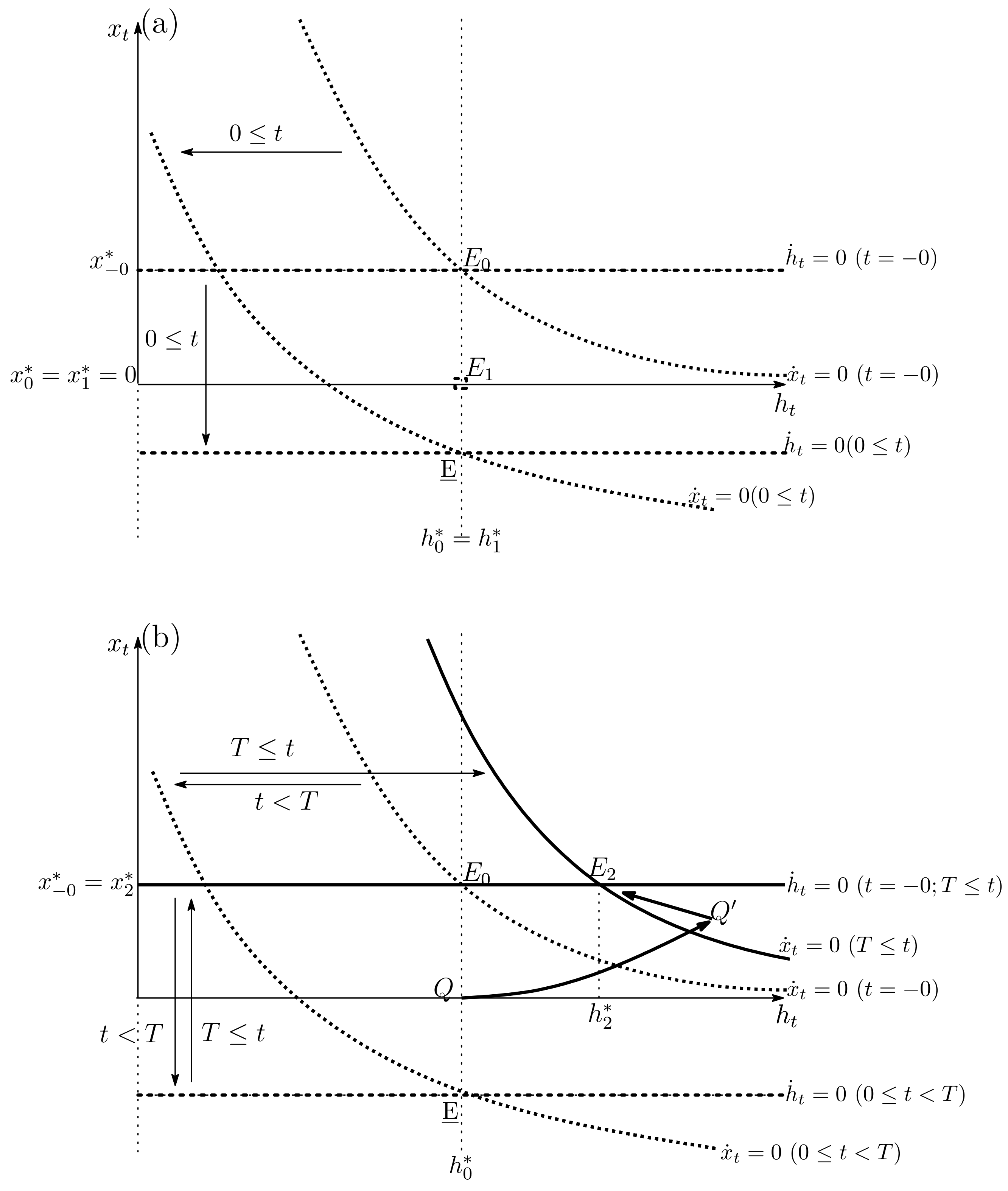
The abovementioned result arises only when the direct distribution of health-related goods does not offset all private spending on health-related goods. In other words, the above case can be seen only when $x_j^{*}>0$. On the contrary, if the government makes a large-scale distribution of health-related goods, such huge public investment may influence HRQOL. Now, we suppose that a huge amount of the distribution of health-related goods is enforced permanently, and hence that the ${\dot{h}}_t=0$ locus moves downward, so that the intersection between the ${\dot{h}}_t=0$ and ${\dot{x}}_t=0$ loci is given by $\underline{E}$ in Figure 4a. Then, a huge amount of public investment leads to $x_0=0$. Since this health policy continues permanently, the zero level of private spending on health-related goods is also kept (i.e., $x_t=0$ for all t). Then, if the economy moves around the long-run equilibrium, we can use Equation (22) under $x_t=x_1^{*}=0$. As a result, by integrating Equation (22), we can obtain $b_t=b_0^{*}=b_1^{*}$ for all t. Finally, noting that the solvency condition guarantees the existence of the long-run equilibrium, the solvency condition leads to $h_0^{*}=h_1^{*}$ because $b_0^{*}=b_1^{*}$. On the contrary, from Equation (20) under $b_1^{*}=b_0^{*}$, $l_1^{*}=l(0,{\eta }_j)$, and $x_1^{*}=0$, we can see that the large amount of public investment crowds out the level of consumption as follows:

$$\frac{\partial \overline{c}}{\partial \eta }=f\left(\overline{k}\right)l_{\eta }-1(<0).$$

(28)

Equations (16a) and (17) do not hold under $x^{*}=0$. We can conclude that $c_{-0}^{*}>c_0^{*}=c_1^{*}$.

As for the temporary enforcement of public investment in HRQOL, the downward jump in consumption remains in the long run. Therefore, after the repeal of the public health policy, the ${\dot{h}}_t=0$ locus returns to the original position, while the ${\dot{x}}_t=0$ locus moves towards the right compared with the original position. As a result, as in Figure 4b, the economy arrives at the new steady state $E_2$ that $h_0^{*}<h_2^{*}$. In sum, the temporary enforcement of public investment in HRQOL generates dynamic behavior in the economy because of a change in the constant level of consumption.

Finally, since one may consider that the assumption of the separability of the utility function is critical to obtain our main findings, we extend the formation of the utility function as a non-separable one to show that our findings are supported in a general form of the utility function as well. For the details, see Appendix E.

6. Discussion

For poor countries that cannot sustain a public health program steadily, it is important to examine the effects of a temporary public health program on HRQOL. In the comparative static analysis, we analytically found that when the price reduction of health-related goods is temporarily enforced, HRQOL deteriorates in the long run. On the contrary, the temporary enforcement of the direct distribution of health-related goods has an insignificant impact on the economy unless the government distributes a huge amount of health-related goods.

To investigate these public policies further, we consider the following three topics. First, we consider an alternative health program with respect to the direct distribution of health-related goods by foreign aid. The reason is that there is a health-related paradox between domestic policies and foreign aid in [41], showing that increased health aid from foreign countries is associated with a statistically significant reduction in infant and child mortality, while the crowding out effect allows the domestic government policy to have a negligible effect on health status. Furthermore, official development assistance from member countries of the Development Assistance Committee of the OECD peaked at $142.6 billion in 2016 and increased by 8.9% compared with 2015. In sum, considering that poor countries largely depend on the assistance of foreign countries, we clarify the role of foreign aid in the form that foreign countries distribute health-related goods. Second, based on our analytical findings, we examine the quantitative impacts of the public health program on HRQOL. Specifically, we are interested in the impacts of the enforcement duration in the policy on the economy, which cannot be investigated analytically. Finally, assuming that $g=g(x_t,\eta )$ with ${\partial }^{2}g(x_t,\eta )/(\partial x_t\partial \eta )>0$, not $g=g(x_t+\eta )$, we re-examine the effects of temporary increase in $\eta$.

6.1. Foreign Aid as an Alternative Way to Directly Distribute Health-Related Goods

We have found that the direct distribution of health-related goods in the form of Equation (4) has trivial impacts because of the crowding out effect unless the government distributes a huge amount of health-related goods. We now assume that the distribution of health-related goods is performed by foreign aid. Then, since residents in the recipient country do not have any tax burden, the budget constraint can be rewritten as

$$\begin{array}{c}\hfill {\dot{\tilde{b}}}_t=r{\tilde{b}}_t+{\tilde{l}}_{t}f\left(k\right)-{\tilde{c}}_t-{\tilde{x}}_t,\end{array}$$

(29a)

where this model is expressed by the variables with the tilde. On the contrary, the evolution of HRQOL is fundamentally the same as in the baseline model:

$$\begin{array}{c}\hfill {\dot{\tilde{h}}}_t=g({\tilde{x}}_t+m)-G\left({\tilde{l}}_t\right),\end{array}$$

(29b)

where m represents the direct distribution of health-related goods by foreign aid.

Following a similar analysis to that in Section 2.2 and Section 3, in the steady state we find that

$$\begin{array}{cc}\hfill & v^{\prime }\left({\tilde{h}}_j^{*}\right)g^{\prime }({\tilde{x}}_j^{*}+m_j)=r{u}^{\prime }\left({\overline{\tilde{c}}}_j^{*}\right),\hfill \end{array}$$

(30a)

$$\begin{array}{cc}\hfill & g({\tilde{x}}_j^{*}+m_j)=G\left(\tilde{l}({\tilde{x}}_j^{*},m_j)\right),\hfill \end{array}$$

(30b)

$$\begin{array}{cc}\hfill & r{\tilde{b}}_j^{*}+\tilde{l}({\tilde{x}}_j^{*},m_j)f\left(k\right)={\overline{\tilde{c}}}_j^{*}+{\tilde{x}}_j^{*},\hfill \end{array}$$

(30c)

$$\begin{array}{cc}\hfill & {\tilde{b}}_{t_0}={\tilde{b}}_j^{*}+{\tilde{\Omega }}_j\left(\frac{{\tilde{\Theta }}_j^s{\tilde{A}}_j^s}{{\tilde{a}}_j^s-r}+\frac{{\tilde{\Theta }}_j^u{\tilde{A}}_j^u}{{\tilde{a}}_j^u-r}\right),\hfill \end{array}$$

(30d)

where ${\tilde{x}}_j^{*}$ has a positive value. As for the function $\tilde{l}({\tilde{x}}_j^{*},m_j)$, we obtain the same signs of the partial derivative: ${\tilde{l}}_x\left(\equiv \frac{\partial {\tilde{l}}_t}{\partial {\tilde{x}}_t}\right)={\tilde{l}}_m\left(\equiv \frac{\partial {\tilde{l}}_t}{\partial m}\right)=\frac{g^{″}({\tilde{x}}_t+m)f\left(k\right)}{(1-\tau )G^{″}\left({\tilde{l}}_t\right)}<0.$

When the original steady state before $t_0=0$ is shown by $\{{\tilde{h}}_0^{*},{\tilde{x}}_{-0}^{*},{\tilde{b}}_0^{*},{\overline{\tilde{c}}}_{-0}^{*}\}$, we similarly denote the steady-state levels under a permanent increase in m by $\{{\tilde{h}}_1^{*},{\tilde{x}}_1^{*},{\tilde{b}}_1^{*},{\overline{\tilde{c}}}_1^{*}\}$ and those under a temporary increase in m by $\{{\tilde{h}}_2^{*},{\tilde{x}}_2^{*},{\tilde{b}}_2^{*},{\overline{\tilde{c}}}_2^{*}\}$. The results are summarized as follows.

Proposition 4.

(i) A permanent increase in m leads to

${\tilde{h}}_1^{*}>{\tilde{h}}_0^{*}$, ${\tilde{x}}_{-0}^{*}>{\tilde{x}}_1^{*}$, ${\tilde{x}}_0>{\tilde{x}}_1^{*}$, ${\overline{\tilde{c}}}_1^{*}={\overline{\tilde{c}}}_0>{\overline{\tilde{c}}}_{-0}^{*}$, and${\tilde{b}}_0^{*}>{\tilde{b}}_1^{*}$. (ii) A temporary increase in m leads to${\tilde{h}}_2^{*}>{\tilde{h}}_0^{*}$, ${\tilde{x}}_{-0}^{*}={\tilde{x}}_2^{*}$, ${\overline{\tilde{c}}}_2^{*}={\overline{\tilde{c}}}_0>{\overline{\tilde{c}}}_{-0}^{*}$, and${\tilde{b}}_0^{*}<{\tilde{b}}_2^{*}$.

Proof. 

See Appendix F. □

When expenditure on the distribution of health-related goods is funded by foreign aid, the government does not impose any tax burden upon residents in the domestic country. Because of the room for budget financing, residents can thus spend on more consumption. This means that ${\overline{\tilde{c}}}_1^{*}>{\overline{\tilde{c}}}_{-0}^{*}$ and ${\overline{\tilde{c}}}_2^{*}>{\overline{\tilde{c}}}_{-0}^{*}$ (i.e., ${\tilde{C}}_m>0$). See Appendix F. Then, the shift in the ${\dot{\tilde{x}}}_t=0$ locus is given by

$$\frac{\partial \tilde{x}}{\partial m}{|}_{{\dot{\tilde{x}}}_t=0,{\tilde{h}}^{*}=\mathrm{const}}=-1+\underset{(\#3)}{\underbrace{\frac{g^{\prime }({\tilde{x}}_j^{*}+m_j)u^{″}\left({\overline{\tilde{c}}}_j^{*}\right)}{g^{″}({\tilde{x}}_j^{*}+m_j)u^{\prime }\left({\overline{\tilde{c}}}_j^{*}\right)}{\tilde{C}}_m}}\gtrless 0,$$

(31a)

where $(\#3)$ has a positive sign. The shift in the ${\dot{\tilde{h}}}_t=0$ locus is

$$\frac{\partial \tilde{x}}{\partial m}{|}_{{\dot{\tilde{h}}}_t=0,{\tilde{h}}^{*}=\mathrm{const}}=-1.$$

(31b)

The comparison of (27) with (31a) and (31b) may be useful to understand the impacts of the crowding out effect. Returning to (27), we concluded that an increase in the direct distribution of health-related goods is perfectly substituted by a decrease in private spending on health-related goods. On the contrary, since external financing by foreign aid does not impose any burden on residents in the domestic country, the downward shift in ${\dot{\tilde{x}}}_t=0$ in (27) shrinks because of the term $(\#3)$ in (31a). As for the ${\dot{\tilde{h}}}_t=0$ locus, the downward shift is the same in (27) and (31b).

Private spending on health-related goods may increase or decrease at time 0 (i.e., ${\tilde{x}}_0\gtrless {\tilde{x}}_{-0}^{*}$) as the direct distribution of health-related goods under foreign aid has two effects on demand for health-related goods. First, there is a substitution effect: an increase in foreign aid leads to a decrease in private spending on health-related goods. Second, there is a wealth effect in the sense that no tax burden exists, which implies that residents can spend more on health-related goods. For instance, if the substitution effect is so large, it seems that they decrease spending on health-related goods; alternatively, if the wealth effect is sufficiently large, they spend more on health-related goods.

Based on Proposition 4, Figure 5a,b show the economic behavior under a permanent increase in m. Looking at Figure 5a, as mentioned above, the initial jump in spending on health-related goods may be downward at point Q or upward at point $Q^{\prime }$, where it holds that ${\tilde{x}}_0>{\tilde{x}}_1^{*}$. After the initial jump, the level of HRQOL monotonically increases towards the new steady state $E_1$ or $E_1^{\prime }$. Then, the level of foreign assets monotonically decreases towards the new steady state.

In what follows, we consider economic behavior under a temporary increase in m. We first analyze the case in which the substitution effect dominates the wealth one. Figure 6a,b correspond to this case, showing that the initial jump in spending on health-related goods is downward at point Q or $Q^{″}$. When private spending on health-related goods jumps from the initial steady state $E_0$ to point Q, its level increases until the removal of foreign aid and then decreases towards the new steady state $E_2$; on the contrary, the level of HRQOL continues to increase over time. Figure 6b shows the movement in foreign assets. Since the economy lies on the stable arm during $t\in [T,\infty ]$, we are concerned about the solvency condition. That is, it holds that sign $\{{\tilde{b}}_T-{\tilde{b}}_2^{*}\}=$ sign $\{{\tilde{h}}_2^{*}-{\tilde{h}}_T\}$. Based on the relationship and Proposition 4, we can thus conclude that after the level of foreign assets increases from $E_0$ to R at time T, it decreases until the new steady state $E_2$. Lastly, it holds that ${\tilde{b}}_2^{*}>{\tilde{b}}_{-0}^{*}$.

On the contrary, suppose that private spending on health-related goods is mostly crowded out from $E_0$ to point $Q^{″}$. Then, such spending decreases at the beginning and begins to increase after the economy goes through point $Q^{″\prime }$. Finally, when foreign aid is removed at time T, the economy arrives at point $Q^{″″}$. Hereafter, the level of HRQOL decreases along the stable path from point $Q^{″″}$ to $E_2$. Figure 6b shows that the level of foreign assets decreases from $E_0$ to $R^{\prime }$ and that after the removal of foreign aid, the level of foreign assets increases towards the new steady state $E_2$.

Next, we consider whether the wealth effect dominates the substitution one, so that private spending on health-related goods jumps upward as in Figure 7. When the initial jump arises from the initial steady state $E_0$ to point Q in Figure 7a, the level of HRQOL increases monotonically during the enforcement of foreign aid; alternatively, the level of spending on health-related goods decreases from points Q to $Q^{\prime }$ and then increases from $Q^{\prime }$ to $Q^{″}$. When foreign aid returns to its original level, the economy just arrives at point $Q^{″}$. After the removal of foreign aid, the level of HRQOL decreases from $Q^{″}$ to the new steady state $E_2$. As shown in Figure 7b, after the level of foreign assets decreases during the enforcement of foreign aid (from $E_0$ to R), it begins to increase from point R towards the new steady state $E_2$.

Suppose that the large jump in spending on health-related goods happens from $E_0$ to $Q^{″\prime }$ as a result of the large wealth effect. This effect raises private spending on health-related goods during time $t\in [0,T)$, and hence the level of HRQOL increases as well. After the removal of foreign aid, the direct impact of the wealth effect does not exist. Therefore, private spending on health-related goods decreases, and thus it holds that ${\tilde{x}}_{-0}^{*}={\tilde{x}}_2^{*}$ at the new steady state $E_2$. In this case, Figure 7b shows that the qualitative movement in foreign assets ($E_0\to R^{\prime }\to E_2$) is the same as that in the abovementioned case ($E_0\to R\to E_2$).

6.2. Numerical Examples

In the above subsection, we analyzed the policy effects on HRQOL theoretically. In this subsection, we check our theoretical findings by employing numerical examples. As seen in Section 5, because the direct distribution of health-related goods by the domestic government does not affect the economy significantly, we assume that ${\eta }_j=0$ over time to focus on the other policy effects. Notice that we omit tilde from each variable in Section 6.2 for viewability because we make use of the model of Section 2 in Section 6.2.1 and the model of Section 6.1 in Section 6.2.2

First, we specify the utility functions as $u\left(c_t\right)=c_t^{1-\sigma }/(1-\sigma )$ and $v\left(h_t\right)=h_t^{1-\varphi }/(1-\varphi )$, where $\sigma (>0)$ and $\varphi (>0)$ show the preference parameters. The production of a single homogeneous commodity is given by the production process $f\left(k_t\right)=A{k}_t^{\xi }$, where A and $\xi$ are the production parameters. While these types of utility and production functions are frequently used, we assume that the functions $g(·)$ and $G(·)$ relate to HRQOL as follows:

$$g(x_j+m_j)=\frac{{(x_j+m_j)}^{1-\alpha }}{1-\alpha },G\left(l_j\right)=\frac{l_j^{1+\beta }}{1+\beta },$$

(32)

where $(0<)\alpha (<1)$ and $\beta (>0)$ are the health parameters. Equation (11) leads to the level of labor supply:

$$l_j={\left(\frac{{\left(x_j+m_j\right)}^{-\alpha }f\left(\overline{k}\right)}{1-{\tau }_j}\right)}^{\frac{1}{\beta }}.$$

(33)

Furthermore, by substituting Equation (33) into Equation (17), we find that the steady-state level of private spending on health-related goods is given by

$$x_j^{*}={\left(\frac{1-\alpha }{1+\beta }\right)}^{\frac{\beta }{\alpha +\beta }}{\left(\frac{f\left(\overline{k}\right)}{1-{\tau }_j}\right)}^{\frac{1+\beta }{\alpha +\beta }}-m_j.$$

(34)

We assume that $x_j^{*}>0$ in the numerical simulation.

The parameter values used in our simulations are:

• The production parameters: $\xi =0.2,A=10,$
• Preference and health parameters: $\sigma =2.5,\varphi =5,\alpha =0.5,\beta =0.5,$
• Interest rate: $r=(\rho =)0.1,\mathrm{or}0.2,$
• Policy parameters: ${\tau }_{-0}=0,m_{-0}=0,$
• Initial values: $b_0=10,$
• The duration of the policy enforcement: $T=0.1,0.2\mathrm{or}0.5.$

Some of these parameters are standard ones: $\xi =0.3$ and $\sigma =1.5$. Because some poor countries have high interest rates to some extent, we assume that $r=0.1$ or $0.2$. In that case, setting $A=10$ yields the fixed values of the capital stock, $k=42.2949$ under $r=0.1$ and $k=17.7828$ under $r=0.2$. As for the health parameters, we assume that the elasticity of marginal utility with respect to consumption is lower than that with respect to HRQOL, $\varphi =3.5$, which supposes that the health-related good is a luxury good for people in developing countries. Next, we set the remaining parameters in the functions $g(·)$ and $G(·)$ as follows: $\alpha =\beta =0.5$. In the baseline, we assume that the duration of the policy enforcement, T, is 0.1, 0.2, or 0.5 in the case of temporary policy changes.

As for the initial values of the state variables $h_0^{*}$ and $b_0^{*}$, we provide the initially given value of foreign assets by $b_0^{*}=10$; however, we do not provide the initial level of HRQOL because the initial economy is at the steady state, namely it must satisfy Equations (16a), (17), (20), and (25). Considering that $b_0=b_0^{*}(=10)$, the value of left-hand side of Equation (25) is zero. If the initial level of HRQOL is freely given, the two values of ${\overline{c}}_{-0}^{*}$ and $x_{-0}^{*}$ at the initial economy must be determined by three Equations (16a), (17), and (20), given $b_0^{*}$ and $h_0^{*}$. Therefore, the number of equations is more than that of variables. Thus, by setting $(h_0^{*},x_{-0}^{*},b_0^{*})$ to satisfy the three Equations (16a), (17), and (20), we determine the initially unique values of $(h_0^{*},x_{-0}^{*},b_0^{*})$.

Table 1. The initial levels of the variables.

	${\mathit{x}}_{-0}^{*}$	${\mathit{l}}_{-0}^{*}$	${\mathit{h}}_0^{*}$	${\mathit{b}}_0^{*}$	${\mathit{c}}_{-0}^{*}$
$r=0.1$	56.147	7.9651	11.276	10	113.29
$r=0.2$	43.295	7.304	8.9093	10	88.59

shows the initial economy in our simulation. Taking account of the difference in the return to capital, we see that a higher interest rate leads to lower levels of the variables $x_{-0}^{*}$, $l_{-0}^{*}$, $h_0^{*}$, and $c_{-0}^{*}$. The reason is that because the return to capital equals the discount rate, future investment is substituted by current consumption. Hence, it is plausible that the long-run levels of spending on health-related goods and consumption are lower, thereby leading to a lower level of HRQOL.

We set the policy parameters $\tau$ and m as follows:

$$\tau =0.05,0.1,0.2,m=0.5,1,5.$$

We suppose that the price reduction is 5%, 10%, or 20%. As for foreign aid, we set $m=0.5$, 1, or 5. When the value of m is related to output $l_{-0}^{*}f\left(k\right)=168.4406$ under $r=0.1$, $m=0.5$ ($m=5$) means that the distribution of health-related goods corresponds to 0.3% ($3\%$) of output. For a detailed explanation of the determination in the steady state, see Appendix G.

6.2.1. Price Reduction

When the price reduction $\tau$ is permanently enforced,

Table 2. The permanent increase in $\tau$.

	$\mathit{r}=0.1$						$\mathit{r}=0.2$
	${\mathit{x}}_0$	${\mathit{x}}_1^{*}$	${\mathit{l}}_1^{*}$	${\mathit{h}}_1^{*}$	${\mathit{b}}_1^{*}$	${\mathit{c}}_1^{*}$	${\mathit{x}}_0$	${\mathit{x}}_1^{*}$	${\mathit{l}}_1^{*}$	${\mathit{h}}_1^{*}$	${\mathit{b}}_1^{*}$	${\mathit{c}}_1^{*}$
$\tau =0.05$	161.3	60.637	8.172	17.968	2.366	112.42	162.21	46.758	7.4937	18.582	2.5998	87.022
$\tau =0.1$	178.62	65.76	8.3959	18.151	2.9792	112.09	180.65	50.708	7.6991	19.16	2.8343	86.77
$\tau =0.2$	229.38	78.468	8.9052	19.226	3.3775	110.19	229.03	60.507	8.1661	20.799	3.0516	85.32

shows the long-run levels of the economic variables. First, as confirmed in Proposition 2, a permanent increase in $\tau$ leads to higher spending on health-related goods and a higher level of HRQOL in the new steady state, which decreases the long-run level of foreign assets. Since the price of consumption commodities increases relatively, a permanent price reduction of health-related goods decreases the level of private consumption. For instance, by setting $\tau =0.05$ under $r=0.1$, the level of HRQOL increases from 11.2764 to 17.968. In other words, when the price reduction of health-related goods falls permanently by 5%, the level of HRQOL increases by around 59%. Noting that $h_0^{*}<h_1^{*}$ leads to $b_0^{*}>b_1^{*}$, the level of foreign assets decreases largely by around 76%. Furthermore, when the rate of $\tau$ is 0.2, the level of HRQOL increases by about 71% (from 11.276 to 19.226) and the level of foreign assets decreases by around 66%. Looking at $r=0.2$ in Table 2, we obtain a consistent finding irrespective of the return to capital. In particular, when the rate of $\tau$ is 0.05, the level of HRQOL increases significantly by over 108% (from 8.9093 to 18.582) and the level of foreign assets decreases by around 74%.

Next, we turn to the temporary increase in $\tau$.

Table 3. (a) The temporary increase in $\tau$, where $r=0.1$; (b) The temporary increase in $\tau$, where $r=0.2$.

	(a)
	$\mathit{r}=0.1$:	${\mathit{x}}_0$	${\mathit{h}}_{\mathit{T}}$	${\mathit{b}}_{\mathit{T}}$	${\mathit{c}}_{\mathit{T}}={\mathit{c}}_2^{*}$	${\mathit{x}}_2^{*}$	${\mathit{l}}_2^{*}$	${\mathit{h}}_2^{*}$	${\mathit{b}}_2^{*}$
$T=0.1$	$\tau =0.05$	252.09	11.971	9.2073	113.28	56.147	7.9651	11.186	9.833
	$\tau =0.1$	280.91	11.999	9.2616	113.28	56.147	7.9651	11.213	9.8898
	$\tau =0.2$	367.02	12.123	9.2945	113.29	56.147	7.9651	11.266	9.9826
$T=0.2$	$\tau =0.05$	252.09	12.416	8.6996	113.27	56.147	7.9651	11.104	9.7378
	$\tau =0.1$	280.91	12.459	8.7922	113.28	56.147	7.9651	11.159	9.8254
	$\tau =0.2$	367.02	12.657	8.8495	113.29	56.147	7.9651	11.259	9.9713
$T=0.5$	$\tau =0.05$	252.09	12.862	8.1914	113.26	56.147	7.9651	11.023	9.6351
	$\tau =0.1$	280.91	12.907	8.3347	113.27	56.147	7.9651	11.117	9.7522
	$\tau =0.2$	367.02	13.164	8.4276	113.29	56.147	7.9651	11.249	9.9622
	(b)
	$\mathit{r}=0.2$:	${\mathit{x}}_0$	${\mathit{h}}_{\mathit{T}}$	${\mathit{b}}_{\mathit{T}}$	${\mathit{c}}_{\mathit{T}}={\mathit{c}}_2^{*}$	${\mathit{x}}_2^{*}$	${\mathit{l}}_2^{*}$	${\mathit{h}}_2^{*}$	${\mathit{b}}_2^{*}$
$T=0.1$	$\tau =0.05$	261.86	10.115	9.078	88.534	43.295	7.304	8.4821	9.7176
	$\tau =0.1$	293.21	10.192	9.1036	88.541	43.295	7.304	8.5421	9.7545
	$\tau =0.2$	375.83	10.4	9.1286	88.556	43.295	7.304	8.6536	9.8269
$T=0.2$	$\tau =0.05$	261.86	10.769	8.5775	88.502	43.295	7.304	8.1702	9.5582
	$\tau =0.1$	293.21	10.885	8.6188	88.516	43.295	7.304	8.2389	9.6259
	$\tau =0.2$	375.83	11.205	8.6584	88.538	43.295	7.304	8.4393	9.7366
$T=0.5$	$\tau =0.05$	261.86	11.071	8.3462	88.49	43.295	7.304	7.9248	9.498
	$\tau =0.1$	293.21	11.198	8.3999	88.503	43.295	7.304	8.072	9.5657
	$\tau =0.2$	375.83	11.563	8.4493	88.528	43.295	7.304	8.3591	9.6864

a shows the case in which $r=0.1$, while Table 3b presents the case in which $r=0.2$. At first, it holds that $x_2^{*}=x_{-0}^{*}$ from Table 1 and Table 3, which means that spending on health-related goods at the new steady state is the same as initially. Furthermore, the equality $x_2^{*}=x_{-0}^{*}$ leads to $l_2^{*}=l_{-0}^{*}$. See $l_{-0}^{*}$ in Table 1 and $l_2^{*}$ in Table 3. For instance, let us suppose that the duration of the policy enforcement, T, is 0.1 under $r=0.1$. Then, we find that the level of HRQOL is given by $h_{0.1}=11.971$ at time $T=0.1$, which increases by 6% relative to its initial level. After the price reduction of health-related goods is removed, the long-run level of HRQOL is lower than its initial level by around 0.8% (from 11.276 to 11.186). Furthermore, the levels of foreign assets at time T and at the new steady state $E_2$ are lower than the original level, as shown in Figure 2.

Table 3a shows that increasing the rate of $\tau$ leads to higher levels of HRQOL and foreign assets at time T and at the new steady state $E_2$. For example, under $T=0.1$, when the rate of $\tau$ increases from 0.05 to 0.2, the level of HRQOL at time T increases by around 1.2% (from 11.971 to 12.123) and the level of HRQOL at the new steady state increases by around 0.7% (from 11.186 to 11.266). Similarly, the level of foreign assets increases by around $0.95\%$ at $T=0.1$ and by around $1.5\%$ at the new steady state $E_2$.

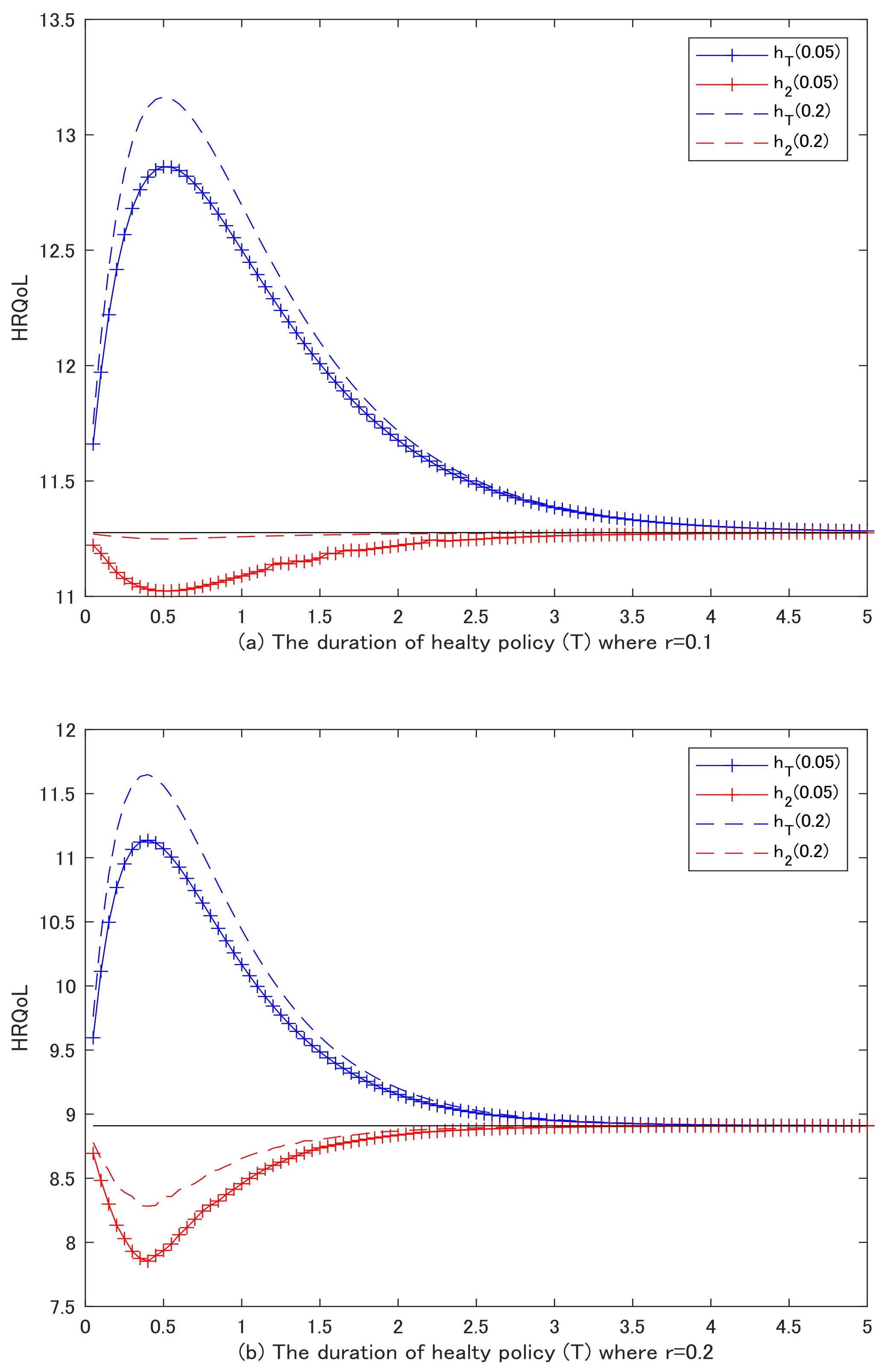
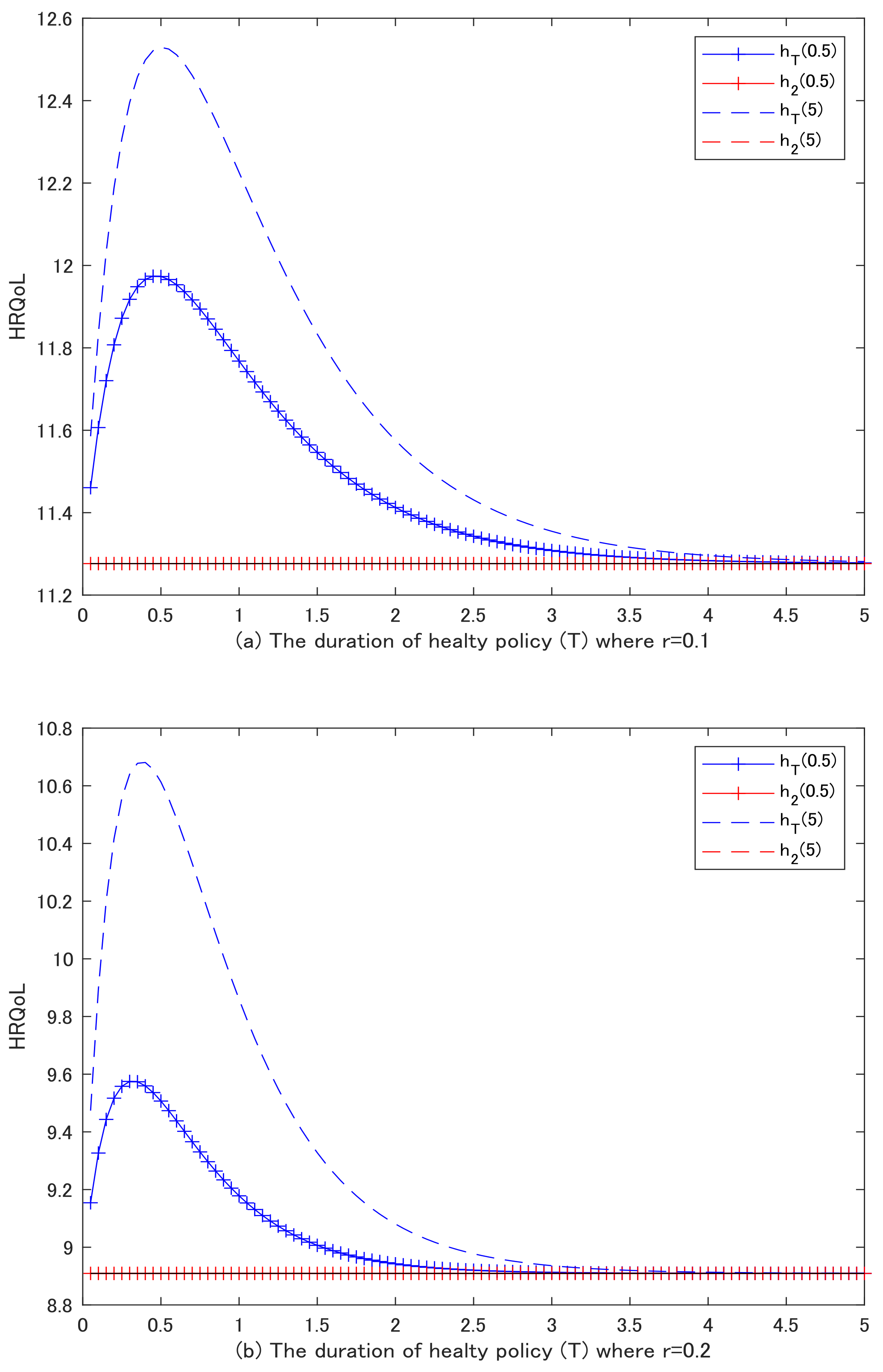
Finally, Figure 8a,b shows the relation between HRQOL and the enforcement duration of the health policy, where $r=0.1$ ($r=0.2$). The x-axis shows the duration of the policy enforcement and the y-axis the level of HRQOL. The blue curves correspond to the levels of HRQOL at time T and the red ones the levels of HRQOL at the new steady state. In addition, the dotted curve depicts the case in which $\tau =0.05$ and the curve with a plus sign depicts the case in which $r=0.2$. Noting that the black line shows the initial level of HRQOL, $h_0^{*}=11.276$, the blue curves are located above the black line, which implies that the levels of HRQOL at time T are more than its initial level. On the contrary, since the red curves are located below the black line, the levels of HRQOL at the new steady state are less than its initial level. Moreover, Figure 8a,b shows that the numerical finding is consistent irrespective of the return to capital.

There are four findings in Figure 8a,b. First, these curves are hump-shaped. As the value of T becomes larger, the extension of the duration has a large impact on the level of HRQOL; furthermore, when the value of T increases greatly, the impact weakens, and finally, it seems that the level of $h_T$ approaches that of $h_0^{*}$. For instance, in Figure 8a there is a mountain/valley peak when the duration of the policy enforcement, T, is around 0.5. In detail, the level of HRQOL at time T increases monotonically as the value of T increases from 0 to 0.5. Furthermore, when the duration of the policy enforcement increases from $T=0.5$, the level of HRQOL at time T becomes smaller. Finally, the blue curve approaches the black line, meaning that the level of HRQOL at time T is close to its initial level. Looking towards the red curves in Figure 8a, the level of HRQOL at the new steady state decreases as the duration of the policy enforcement increases until $T=0.5$, and it begins an upward tread when the duration further increases, approaching its initial level of HRQOL. Second, when the level of HRQOL takes a higher value at time T, it takes a lower value at the new steady state. For instance, when T is around 0.5, the level of HRQOL takes its highest value at time T; alternatively, it takes its lowest value at the new steady state. Remembering that the level of consumption does not return to the original level after the removal of the health policy, we can thus presume that the indirect impact of consumption has the largest impact around $T=0.5$ in Figure 8a. Third, comparing $\tau =0.05$ with $\tau =0.2$, a higher rate of $\tau$ leads to higher levels of HRQOL at time T and at the new steady state. For instance, the dotted curves are always above the curve with a plus sign. Finally, the red curves in Figure 8b move considerably, implying that when the interest rate is higher, the temporary price reduction has a large impact on HRQOL in the new steady state. In other words, since a higher interest rate means a higher discounting rate, future consumption is substituted by the current one. This impact of consumption is larger under a higher discounting rate, meaning that the level of HRQOL in Figure 8b decreases largely at the new steady state.

6.2.2. Foreign Aid

Figure 5 shows the permanent increase in foreign aid (the distribution of health-related goods by foreign aid). As mentioned in Section 5 and Section 6.1, foreign aid has crowding out effects on private spending on health-related goods. For instance,

Table 4. The permanent increase in m.

	$\mathit{r}=0.1$						$\mathit{r}=0.2$
	${\mathit{x}}_0$	${\mathit{x}}_1^{*}$	${\mathit{l}}_1^{*}$	${\mathit{h}}_1^{*}$	${\mathit{b}}_1^{*}$	${\mathit{c}}_1^{*}$	${\mathit{x}}_0$	${\mathit{x}}_1^{*}$	${\mathit{l}}_1^{*}$	${\mathit{h}}_1^{*}$	${\mathit{b}}_1^{*}$	${\mathit{c}}_1^{*}$
$m=0.5$	107.9934	55.6469	7.9651	14.2068	7.0341	113.4972	93.6203	42.7952	7.304	11.76	8.4513	88.7806
$m=1$	124.1375	55.1469	7.9651	15.555	5.2586	113.8196	113.2568	42.2952	7.304	13.5254	7.1158	89.0135
$m=5$	130.4297	51.1469	7.9651	16.5563	3.7724	117.671	132.7088	38.2952	7.304	16.5241	4.1875	92.4278

shows that under $r=0.1$, setting $m=0.5$ leads to a decrease of around 0.9% in private spending on health-related goods (from 56.147 to 55.547). Furthermore, when the value of m is set at 5, private spending on health-related goods further declines by around 8% (from 55.647 to 51.147). In what follows, the level of labor supply is constant under the functions of our simulation. Concretely, by using the first-order condition in labor supply and Equation (30b), we can derive $x_1^{*}={\left(\frac{1-\alpha }{1+\beta }\right)}^{\frac{\beta }{\alpha +\beta }}f{\left(\overline{k}\right)}^{\frac{1+\beta }{\alpha +\beta }}-m.$ In addition, labor supply can be derived by $l_1^{*}={\left(x_1^{*}+m\right)}^{-\frac{\alpha }{\beta }}f{\left(\overline{k}\right)}^{\frac{1}{\beta }}$. As a result, substituting $x_1^{*}$ into $l_1^{*}$ means that m does not affect labor supply. Furthermore, unlike the distribution of health-related goods by the domestic government, in the case of foreign aid, the domestic government does not impose any taxation on domestic residents. Hence, residents can spend to raise private consumption. In detail, when $m=0.5$ under $r=0.1$, the level of consumption increases by 0.2%. Finally, the level of HRQOL in the new steady state increases by around 26% (from 11.276 to 14.207); alternatively, the level of foreign assets decreases by around 30%. The qualitative impacts of foreign aid are thus the same irrespective of the interest rate.

Next,

Table 5. (a) The temporary increase in $\tau$, where $r=0.1$; (b) The temporary increase in $\tau$, where $r=0.2$.

	(a)
	$\mathit{r}=0.1$:	${\mathit{x}}_0$	${\mathit{h}}_{\mathit{T}}$	${\mathit{b}}_{\mathit{T}}$	${\mathit{c}}_{\mathit{T}}={\mathit{c}}_2^{*}$	${\mathit{x}}_2^{*}$	${\mathit{l}}_2^{*}$	${\mathit{h}}_2^{*}$	${\mathit{b}}_2^{*}$
$T=0.1$	$m=0.5$	155.8174	11.6065	9.6659	113.2938	56.1469	7.9651	11.2764	10.0000
	$m=1$	186.7466	11.7407	9.4854	113.2938	56.1469	7.9651	11.2764	10.0000
	$m=5$	202.0166	11.8347	9.3415	113.2938	56.1469	7.9651	11.2764	10.0000
$T=0.2$	$m=0.5$	155.8174	11.8073	9.4627	113.2938	56.1469	7.9651	11.2764	10.0000
	$m=1$	186.7466	12.0302	9.1646	113.2938	56.1469	7.9651	11.2764	10.0000
	$m=5$	202.0166	12.1885	8.9242	113.2938	56.1469	7.9651	11.2764	10.0000
$T=0.5$	$m=0.5$	155.8174	11.9732	9.2947	113.2938	56.1469	7.9651	11.2764	10.0000
	$m=1$	186.7466	12.2933	8.8731	113.2938	56.1469	7.9651	11.2764	10.0000
	$m=5$	202.0166	12.5293	8.5222	113.2938	56.1469	7.9651	11.2764	10.0000
	(b)
	$\mathit{r}=0.2$:	${\mathit{x}}_0$	${\mathit{h}}_{\mathit{T}}$	${\mathit{b}}_{\mathit{T}}$	${\mathit{c}}_{\mathit{T}}={\mathit{c}}_2^{*}$	${\mathit{x}}_2^{*}$	${\mathit{l}}_2^{*}$	${\mathit{h}}_2^{*}$	${\mathit{b}}_2^{*}$
$T=0.1$	$m=0.5$	139.0812	9.3266	9.7733	88.5904	43.2952	7.304	8.9093	10.0000
	$m=1$	176.0275	9.5507	9.5992	88.5904	43.2952	7.304	8.9093	10.0000
	$m=5$	214.6666	9.8884	9.2526	88.5904	43.2952	7.304	8.9093	10.0000
$T=0.2$	$m=0.5$	139.0812	9.5168	9.67	88.5904	43.2952	7.304	8.9093	10.0000
	$m=1$	176.0275	9.8626	9.4044	88.5904	43.2952	7.304	8.9093	10.0000
	$m=5$	214.6666	10.4047	8.8585	88.5904	43.2952	7.304	8.9093	10.0000
$T=0.5$	$m=0.5$	139.0812	9.5068	9.6754	88.5904	43.2952	7.304	8.9093	10.0000
	$m=1$	176.0275	9.9044	9.3783	88.5904	43.2952	7.304	8.9093	10.0000
	$m=5$	214.6666	10.5981	8.7109	88.5904	43.2952	7.304	8.9093	10.0000

shows the numerical results with respect to the effects of a temporary increase in m. Table 5a presents the case in which $r=0.1$ and Table 5b shows the case in which $r=0.2$. Spending on health-related goods at the new steady state is the same as at its original level, namely $x_2^{*}=x_{-0}^{*}$. Furthermore, this means that $l_2^{*}=l_{-0}^{*}$. The numerical results support the findings in Proposition 4. Alternatively, we turn to the new steady state after the removal of foreign aid. Looking at $h_2^{*}$ and $b_2^{*}$ in Table 5a, we find that foreign aid, m, has insignificant impacts on HRQOL and foreign assets at the new steady state because the upward jump in private consumption is very small. In other words, an increase in foreign aid can be substituted by a decrease in private spending on health-related goods. Hence, the level of consumption does not increase largely at time 0, which corresponds to Table 5a that $c_{-0}^{*}=c_T=c_2^{*}$; however, in fact, the level of consumption increases slightly below 0.1%. Therefore, after the removal of foreign aid, only a slight increase in consumption affects the long-run levels of HRQOL and foreign assets. As a result, the levels of $h_2^{*}$ and $b_2^{*}$ are similar to those of $h_0^{*}$ and $b_0^{*}$ in Table 1. These trends are the same even if the interest rate rises.

Finally, Figure 9a,b plots the level of HRQOL at time T and at the new steady state $E_2$ as in Figure 8a,b. They show that when the distribution of health-related goods is enforced until T, HRQOL at time T takes a high value. Alternatively, the long-run levels of HRQOL are almost all the same as the initial levels, which do not change regardless of the duration of the policy enforcement. In addition, this finding is consistent irrespective of the interest rate.

6.3. The Complementary Relationship between $x_t$ and $\eta$

Apart from the direct distribution of the health-related goods by government in the baseline set-up, we assume the complementary relationship between the public and the private health investment as follows:

$$g=g(x_t,\eta ),\mathrm{where}\frac{{\partial }^{2}g(x_t,\eta )}{\partial x_t\partial \eta }\equiv g_{x\eta }(x_t,\eta )>0.$$

(35)

The perfect substitution between the private and the public health investment, $g=g(x_t+\eta )$ represents the direct distribution of health-related goods by government, while Equation (35) means that the public health investment cannot be substituted, but it generates positive externalities such as sanitation, DDT sparying for malaria control etc. In sum, the content of government assistance differs substantially.

Since the perfect substitution of $x_t$ and $\eta$ is not held, Equation (13a) is not held. Concretely, they are given by:

$$l_x=\frac{g_{xx}(x_t,\eta )G^{\prime }\left(l_t\right)}{g_x(x_t,\eta )G^{″}\left(l_t\right)}(<0),l_{\eta }=\frac{g_{x\eta }(x_t,\eta )G^{\prime }\left(l_t\right)}{g_x(x_t,\eta )G^{″}\left(l_t\right)}(>0).$$

As a result, the temporary increase in $\eta$ have the different impact on HRQOL qualitatively. While the public health investment, $\eta$ does not have any impacts on the foreign asset under the perfect substitution in the baseline model, it impacts the foreign asset as follows:

$$\frac{\partial b^{*}}{\partial \eta }=\underset{(+)}{\underbrace{\frac{G^{\prime }{\left(l^{*}\right)}^2\left(\frac{G^{″}\left(l^{*}\right)G\left(l^{*}\right)}{G^{\prime }{\left(l^{*}\right)}^2}-\frac{g_{xx}(x^{*},\eta )g(x^{*},\eta )}{g_x{(x^{*},\eta )}^2}\right)}{r(g_x(x^{*},\eta )-G^{\prime }\left(l^{*}\right)l_x)G^{″}\left(l^{*}\right)}}}(g_x(x^{*},\eta )-g_{\eta }(x^{*},\eta )).$$

(36)

Importantly, the public health investment $\eta$ now has the indirect impact on the level of consumption by changing the foreign asset. In detail, if $g_x(x^{*},\eta )>g_{\eta }(x^{*},\eta )$, then the level of foreign asset increases in the long run, concluding that the level of private consumption increases. As a result, the temporary enforcement of $\eta$ makes the level of HRQOL increased. On the other hand, when $g_x(x^{*},\eta )<g_{\eta }(x^{*},\eta )$, the lower level of foreign asset leads to a lower level of consumption, thereby showing that the level of HRQOL is deteriorated in the long run.

7. Conclusions

In this study, we have analyzed the effects of public policies in health on HRQOL in a dynamic model of a small open economy. We have found that the temporary effects of public policies (a price reduction of health-related goods and the direct distribution of such goods) by the domestic government do not have any positive impacts on HRQOL in the long run. On the contrary, when the price reduction of health-related goods is permanently enforced, or when health-related goods are temporarily/permanently distributed by foreign aid, HRQOL increases over time and the long-run level of HRQOL is greater than its original level.

The findings of this study have some interesting policy implications. They show that the domestic government should not enforce health policies from a short-term perspective. To improve HRQOL, the domestic government should rather implement a permanent price reduction of health-related goods such as high-quality food and drink or medicine. Furthermore, if the domestic government tries to distribute health-related goods, it should ask for foreign aid because the domestic enforcement of the distribution of health-related goods does not influence HRQOL owing to the crowding out effect.

In analyzing the permanent and temporary effects of public policies, we have supposed the equilibrium path under the assumption of perfect foresight. Alternatively, because people in poor countries cannot accurately recognize the governance issues specific to poor countries, including such topics as democratization, corruption control, capacity-building, and electoral and judicial systems, we could improve our analysis by considering an economy where foresight is imperfect, which is left for future studies.