Article

Role of Farmers’ Risk and Ambiguity Preferences on Fertilization Decisions: An Experiment

by
Camille Tevenart
1,2 and
Marielle Brunette
1,2,*
1
Université de Lorraine, Université de Strasbourg, AgroParisTech, CNRS, INRAE, BETA, 54000 Nancy, France
2
Climate Economics Chair, 75002 Paris, France
*
Author to whom correspondence should be addressed.
Sustainability 2021, 13(17), 9802; https://doi.org/10.3390/su13179802
Submission received: 29 June 2021 / Revised: 10 August 2021 / Accepted: 27 August 2021 / Published: 31 August 2021

Abstract

:
In the context of climate change, the agricultural sector offers a large number of mitigation possibilities through diverse practices, such as the reduction of pollutant inputs. However, most farmers do not adopt the mitigation practices recommended, including the reduction of nitrogen fertilization. At the same time, various uncertainties characterize agricultural production, so that the farmer’s risk and ambiguity preferences may be potential determinants to the adoption of mitigation practices. In this context, the objective of the article is to determine if the farmer’s risk and ambiguity preferences explain (or not) the fertilization decision. A questionnaire was submitted to French farmers to elicit risk and ambiguity preferences through lottery choices, and ask questions about fertilization. Two regressions were realized, the first to explain the total fertilization and the second to identify the determinants of the first fertilization application. The results reveal that respondents were mostly risk-averse and ambiguity-neutral. In addition, risk and ambiguity aversion impact fertilization practices through diverse drivers in opposite directions. Indeed, being risk-averse is associated with a lower level of total fertilization, whereas ambiguity aversion has a positive and significant impact on the level of fertilization at the first application. This last result highlights the need to reduce the uncertainty farmers face.
JEL Classification:
D81; Q12

1. Introduction

Reducing greenhouse gas (GHG) emissions in the agricultural sector is a major environmental policy challenge in France, where the sector was responsible for 20.4% of the total GHG emissions in 2017 [1]. The agricultural sector, in association with the forest sector, is the main sector capable of sequestering atmospheric carbon and consequently representing a great potential for mitigation. Mitigation practices are proposed to farmers in the context of the European Common Agricultural Policy (CAP). They encourage farmers to diversify their activities, to integrate leguminous crop, to improve land rotation, to develop better links between effective livestock feeding and vegetable protein production, and, above all, to limit the use of pollutant inputs. In this context, reducing synthetic nitrogen fertilization or improving fertilization efficiency is an important mitigation strategy. Reducing the total fertilizer application on parcels and cutting back on the first application in the case of fertilization splitting are two important mitigation practices associated with synthetic nitrogen fertilization. A seminal study on French farmers’ practices and economic characteristics showed that these practices may be associated with negative abatement costs [2]. However, it is often difficult for farmers to implement these mitigation practices, even when they may benefit from them [2]. Several determinants of non-adoption have been identified in the literature. For example, the level of education and farm size are the most reliable variables that appear to significantly positively impact adoption. Hidden costs linked to the existence of uncertainty may be another determinant. Indeed, the adoption of new practices generates production uncertainty in relation to farmer’s profits. In addition to production uncertainty, a price uncertainty may also appear. However, as the mitigation practice considered (fertilization) does not imply a change of the agricultural product or a change of market, the article only focused on production uncertainty. The farmers are dubious of the efficiency of the practices, and the resulting outcome is uncertain. Changing farmers’ habits may be difficult, especially because the reduction of fertilization is associated with uncertain effects on the profit. As a consequence, farmers’ preferences toward risk and ambiguity should also play a role in this adoption process.
Following the modeling approaches of References [3,4,5], inter alia, the use of an input by a producer can be impacted by risk if the input is risk-increasing or decreasing (in yields). The impact depends on the producer’s risk preferences. In other words, a risk-averse agent will use less of a risk-increasing input than a risk neutral one, and vice versa. This result has been specifically extended in the case of input use and agricultural policies by Leathers and Quiggin [6]. These authors show that a policy can be partly inefficient if the risks associated with the input and producers’ preferences toward risk are not taken into account. For instance, taxing a risk-increasing polluting input in order to discourage its use by farmers can lead to disappointing results because risk-averse farmers can try to maintain a sufficiently high level of its use to avoid risk. This phenomenon can explain why yield risk and risk preferences are hidden costs of pollution policies, especially for agricultural policies, leading to low levels of participation.
The relationships between nitrogen fertilization and risk are well-documented in empirical studies that especially use revealed preference methods or agronomic simulations. Stuart et al. [7] show that applying more nitrogen fertilizer is a risk-decreasing activity, and depends on farmers’ perceptions about risk and their trust in the information provided about fertilization reduction. Financial insertion and background risks, as well as the level of competition and the dependency toward contractors, create risks that prevent farmers from reducing their use of nitrogen fertilizer to maintain a sufficient level of yields. Sheriff [8] shows that all farmers set a nitrogen fertilizer rate according to yield expectation, independently of risk preferences, meaning that uncertainty impacts this rate. Moreover, risk aversion and risk perception impact fertilizer use by farmers, as observed by Pope and Kramer [3], i.e., it depends on the risk-decreasing or risk-increasing nature of the input. Bontems and Thomas [9] studied the role of risk aversion and additional information about nitrogen fertilizer applications. They found that a large proportion of their sample of farmers was risk-averse, as well as that risk aversion led to an over-fertilization that accounted for an average of 7.1% of total fertilizer costs per hectare. The value of information, associated with the practice of fertilization splitting and observation of nitrogen availability between splits, accounts for 23.53% of fertilizer costs per hectare. Dequiedt and Servonnat [10] developed the mathematical conditions in which risk aversion would lead to higher rates of fertilization. They empirically tested their results and found that large proportion of French farmers was risk-averse and that these preferences led to 29.4% more nitrogen applications per hectare. This accounts for approximately €75.8/ha and increases the marginal abatement costs of fertilization reduction. Gandorfer et al. [11] studied the gains that farmers would receive if extension agents’ application recommendations took risk and risk aversion into account. Taking different risk measures into consideration, they computed the optimal level of nitrogen rates in different scenarios (in regard to risk aversion) in order to calculate certainty equivalents in the same way as objective yields. Among their results, they found that fertilization, in particular, decreases the probability of negative profits and, in the case of high-risk aversion scenarios, the consideration of risk premiums leads to an average gain per hectare for the farmers. Monjardino et al. [12] also show that risk and risk preferences significantly modify the level of optimal nitrogen fertilization to be applied in order to close the gap between certain yield goals and actual yields. More recently, Meyer-Aurich and Karatay [13] concludes that, in most of their experimental sites, farmer’s risk aversion do not seem to be a strong argument to apply less N fertilizer. The same conclusion is obtained in another article testing the effectivity and cost efficiency of a tax on nitrogen fertilizer [14]. Finally, two recent papers dealing with this problematic in China [15,16] show that the farmer’s risk aversion is associated with a higher level of fertilization. Globally, the theoretical results of the modeling approaches are often validated by empirical studies that show that the level of nitrogen fertilization is impacted by risk perception, risk preferences and arbitrage between yield means and variance. This relationship depends on natural conditions but is relatively robust in one direction: risk aversion seems to encourage farmers to apply more fertilizers on their crops, consequently increasing the cost of reducing applications.
More recently, another category of literature has emerged, based on experimental economics, and proposes to elicit risk and ambiguity aversion parameters through simple lottery choices. By directly measuring risk and ambiguity preferences through experiments, it is possible to isolate these attitudes from other behavioral parameters in a controlled environment. This, therefore, prevents some endogeneity biases related to the simultaneous contribution of perceptions, context and individual preferences to the final decision. Binswanger [17] was the first to submit lotteries to a sample of farmers in order to elicit their risk preferences. The experiment presents a comparison of lotteries from the less to the riskier, and asks farmers to choose their preferred lotteries. The more they akin to risky lotteries, the more risk-loving they are, and vice versa. This Ordered Lottery Selection (OLS) procedure was later generalized by Eckel and Grossman [18]. Binswanger found that Indian farmers were generally risk-averse, as well as that this can have an influence on many different aspects (investment, credit, innovation adoption, etc.). This initial research served as an impulse in the literature, with the subsequent appearance of several elicitation procedures. One of the best-known procedures, the Multiple Price List (MPL) method, was popularized by Holt and Laury [19]. The idea is to submit ten paired-lottery choices to the subjects, and to observe the switching point, i.e., the choice for which they switch from the safe option to the risky one. This switching point then makes it possible to infer a coefficient of relative risk aversion according to the specification of the utility function adopted. This MPL method has already been used to elicit the farmers’ risk preferences. Reynaud and Couture [20] implemented an experiment with 30 French farmers whose aim was to compare three different elicitation procedures, including the MPL. They show that the estimate of risk aversion is dependent on the procedure and the context. Bocquého et al. [21] conducted an experiment on a sample of 100 French farmers and showed that they exhibited attitudes in accordance with expected utility preference assumptions, as well as that they were risk-averse. This MPL procedure was then extended to ambiguity aversion elicitation by Chakravarty and Roy [22]. Their respondents were risk-averse but ambiguity-neutral in the gain domain, and risk-seeking and ambiguity-seeking in the loss domain. Bougherara et al. [23] elicited the risk and ambiguity preferences of 197 French farmers and showed that they are, on average, risk- and ambiguity-averse. The same result was obtained for farmers from other countries, such as Ethiopia, for example [24].
The estimates provided by experimental economics are often used to explain real agricultural decisions. These studies provided divergent results. Ghadim et al. [25] showed that Australian farmers adopt new crops depending on their risk aversion, risk perceptions, and the perceived covariance between the yields of the different crops. Le Cotty et al. [26] found that impatient farmers tend to secure their current consumption by fertilizing more if they are risk-averse, while patient farmers do the reverse if they are risk-averse because they need to smooth their consumption over time. Using a Holt and Laury experiment, Hellerstein et al. [27] found that more risk aversion led to less diversification and less likelihood to adopt an insurance contract. Liu [28] showed that risk aversion can lead to significant delay in adoption of new varieties of crops. Engle-Warnick et al. [29] and Barham et al. [30] both observed with experiments (in Peru and in the U.S., respectively) that ambiguity aversion decreases the probability to adopt a new crop variety if farmers are not sure of the associated distribution of yields or if the new variety increases the level of ambiguity concerning yields. In the latter, the authors even show that risk aversion has no impact on the adoption of risk-decreasing crops, suggesting that ambiguity alone can sometimes have an effect per se.
In this context, the addressed question is the following: What is the impact of farmers’ preferences towards risk and ambiguity on fertilization choices? To answer to this question, risk and ambiguity aversion parameters were elicited through simple lottery choices (MPL method) and then used as potential explanatory variables for farmers’ fertilization choices. The idea is that hidden costs linked to the existence of uncertainty may (partially) explain the non-adoption of fertilization reduction to mitigate climate change. Finally, experimental data on risk and ambiguity aversion are combined with real data on the fertilization decisions. The results of the lottery choices experiment reveal that the respondents are mostly risk-averse and ambiguity-neutral. In addition, the results of the regressions indicate that risk aversion has a significant and negative impact on total fertilization, whereas ambiguity aversion has a significant and positive impact on the level of fertilization, at the first application.
The rest of the paper is organized as follows. Section 2 presents the questionnaire and the methods. The results are presented in Section 3. Section 4 is devoted to a discussion, and Section 5 provides a conclusion of the paper.

2. Materials and Methods

The questionnaire was divided into three parts (see Appendix A). The first part consists of lottery choices to elicit risk aversion and ambiguity aversion parameters. The second part is related to the farmers’ practices in terms of fertilization, and it also contains some information about their property. The last part is dedicated to socio-demographic characteristics.
The questionnaire was submitted to a sample of 45 French farmers from four French agricultural cooperatives. The size of the sample is often small when dealing with “real subjects”. It may be compared with the sample of 30 French farmers of Reynaud and Couture [20] and to the sample of 42 French private forest owners of Brunette et al. [31]. Before diffusion, the questionnaire was tested among different populations: farmers, agronomic engineers and researchers. The questionnaire was completed during meetings organized by the cooperatives, between November 2018 and March 2019. The meetings took place in six different departments: Drôme, Meuse, Tarn, Charente-Maritime, Isère, and Meurthe-et-Moselle. The researchers were present during the meeting to present the questionnaire and answer to any potential questions from the farmers.

2.1. Part 1 of the Questionnaire: Elicitation of Preferences

The preferences are elicited through a MPL method, as proposed by Holt and Laury [19] for risk, and Chakravarty and Roy [22] for ambiguity. Appendix B presents the lottery choices under risk and ambiguity. For each task, individuals are presented with ten decisions between two lotteries (Option A and Option B). For each decision, the subject has to choose between a safe option (Option A) and a risky one (Option B) for risk, and between a risky option (Option A) and an ambiguous one (Option B) for ambiguity. The number of safe choices makes it possible to infer a coefficient for the relative risk aversion coefficient assuming a power utility function, such as: U ( x ) = x r , where r is the relative risk aversion coefficient, and x is the wealth. The expected utility is given by E u ( x ) = p U ( x ) , where p is the objective probability associated with a set of risky outcomes. Table 1 presents this classification. Under the same assumption, Table 2 presents the classification for ambiguity aversion consistent with Chakravarty and Roy [22]. The KMM model [32] was used to represent ambiguity preferences through a ϕ function representing the distortion of the value function according to ambiguity preferences. Given s, the subjective probability belief over a set of ambiguous outcomes, the total expected value function over outcomes can be written as V ( x ) = s ϕ [ E u ( x ) ] , with ϕ ( z ) = z a . The concavity of U gives the level of risk aversion, while the concavity of ϕ gives the level of ambiguity aversion.
Two indicators may be extracted from these tables. The first one is the number of safe choices to represent risk aversion and the number of risky choices to represent ambiguity aversion. In both cases, the higher the number is, the higher the strength of the aversion will be. The second indicator that may be computed is an individual’s average risk and ambiguity coefficient. Indeed, using the center of the interval allows to attribute the corresponding coefficient to each subject. These two indicators are then used as a farmer’s characteristic and considered as a potential explanatory variable for fertilization choices.

2.2. Order Effect and Incentives

The first part of the questionnaire used methodology from experimental economics to elicit farmer’s preferences. In this part, financial incentives are not allowed as is traditionally done in such tasks in experimental economics, especially in lab experiments. However, the farmers were informed that they would receive the results of the study. In the literature, References [33,34] showed that, since questions are related to simple lottery choices, monetary incentives do not seem to significantly affect the decisions. In the same vein, some papers show the absence of differences in terms of decisions between lottery choices using hypothetical or real payoffs [35,36]. Finally, as indicated by Dohmen et al. [37], hypothetical choices still represent good predictors of risk preferences. In this context, a bias resulting from not using financial incentives is not expected.
Another concern when using elicitation tasks from experimental economics is the order effect, i.e., the order in which the subjects respond to the various tasks. In order to control for order effect, half of the distributed questionnaire first began with the elicitation of preferences towards risk, followed by the elicitation of ambiguity preferences, and the opposite for the other half.

2.3. Parts 2 and 3 of the Questionnaire: Fertilization and Socio-Demographic Characteristics

The survey specifically focuses on the biggest parcel of the farm (except grasslands). The biggest parcel is most likely to host the farm’s main crop during the agricultural season and is the crop from which the farmer expects to earn the majority of his/her profits (scale effect, intensity effect). Specific questions associated with parameters that can explain nitrogen needs and nitrogen fertilization decisions are asked in order to provide relevant control variables: spreadable area on the parcel, type of previous crop, soil type, potential organic fertilizer use, and fertilizer tillage. Questions concerning parcel location (department, municipality), the farmer’s status (owner, tenant), and the potential cropping contract are also asked.
The actual and expected yields are crucial for the farmers since the risk they would face relative to fertilization is related to how they intend to reach their yield objective. Since actual yields give us vague general information about the level of efficiency of fertilization decisions, the yield goal before the end of the season is a proxy of what yields could have been expected at the beginning, and the difference between both is a proxy of the actual impacts that farmers face with respect to their crops. This proxy is expected as a potential explanatory variable of the fertilization level, in interaction with risk and ambiguity preferences.
Synthetic nitrogen fertilization and its potential N 2 O emission depends on multiple parameters: the quantity of fertilizer applied, the spreading method used, and the way spreading is broken down according to plant needs, where all of these elements are related to the current regulation on nitrogen fertilization. All these elements are explored in order to have a complete view of how synthetic nitrogen can be used. These elements are associated with the recommendations that farmers received about them from their cooperative agent. This last part was of particular importance for the cooperative partners in terms of monitoring and evaluating their activities. This section on fertilization can, therefore, be summed up as follows. In order to test the way that risk and ambiguity preferences can impact N 2 O emissions from synthetic nitrogen fertilization and the capacity to follow the official recommendations about fertilization, the questionnaire attempted to identify quantity and quality variables related to actual fertilization and recommendations in order to construct different variables.
In order to gather more control variables, farmers were asked about the amount of money they receive from CAP subsidies (and the specific part associated with “green” behaviors), if they had opted for an optional yield insurance contract, the total area of their farm and their possible participation in a farmer’s union.
In the last part, classical questions were asked about socio-demographic variables that can impact risk and ambiguity preferences, as well as the global economic behaviors of the farmers. Age, marital status, education, and revenues (inter alia) were also recorded. The survey is totally anonymous, in order to ensure farmers that their response concerning fertilization (a sensitive topic) will not be associated with them.

3. Results

3.1. Elicitation of Risk and Ambiguity Preferences

In the sample (N = 35), the average Number of Safe Choices (NSC-risk) is 6, while the average Number of Risky Choices (NRC-ambiguity) is around 5. The majority of the respondents are risk-averse (70.27%), whereas 14.86% of farmers are risk-neutral, and the remaining 14.86% are risk-loving. The majority of the respondents are ambiguity-neutral (38.24%) and ambiguity-loving (38.24), and 23.5% are ambiguity-averse (34 non-responses). Each number of safe (risky) choices corresponds to a range of coefficients of risk (ambiguity) aversion. A coefficient is attributed to each number of safe (risky) choices by taking the midpoint of each class, so that each respondent has a coefficient. For the extreme categories, 2 and −2 are assumed under risk, such as Reynaud and Couture [20], which correspond to 2.55 and −0.75 under ambiguity if the same computation method is considered. The average coefficient of risk aversion is 0.615 (prevalence of risk aversion), and the average coefficient of ambiguity aversion is 0.91 (close to ambiguity neutrality).
These results are in line with the findings of Bougherara et al. [23] for French farmers’ risk aversion (0.614), but not for ambiguity aversion (0.722), where the respondents were more ambiguity-averse. The results are very close from those of Barham et al. [30] that found a prevalence of risk aversion preferences in terms of population proportion, and 38% of ambiguity neutrality, 38% of ambiguity-loving, and 24% of ambiguity aversion on a sample of Midwestern (U.S.) farmers. More generally, risk aversion and ambiguity neutrality is in line with the results of Chakravarty and Roy [22] on a sample of Indian students. The good fit of the measures with some results from this previous research is an important outcome in terms of repeatability and external validity of the elicitation methodology.
A categorical variable is constructed with three modalities: if the respondent is risk(ambiguity)-loving, it takes the value of 1; if the respondent is risk(ambiguity)-neutral, it takes the value of 2; if the respondent is risk(ambiguity)-averse, it takes the value of 3. The modality 2 is attributed if the farmer made four safe choices in the risk experiment and five risky choices in the ambiguity experiment. If the answer is below this neutrality number, the farmer is assumed to be risk(ambiguity)-loving, and the farmer is assumed to be risk(ambiguity)-averse if the answer is above this neutrality number. Below is the cross table (Table 3) of risk and ambiguity preferences according to these categories (N = 45).
The proportion (frequencies and percent) in each crossed modality may be observed. It seems that being risk-averse and ambiguity-averse is linked. Independence tests are performed that all failed to reject the independence hypothesis: both variables cannot be considered as significantly dependent. Pairwise Pearson correlations estimations are proposed in Appendix C that reinforce the conclusions about correlation between risk and ambiguity measures.

3.2. Descriptive Statistics

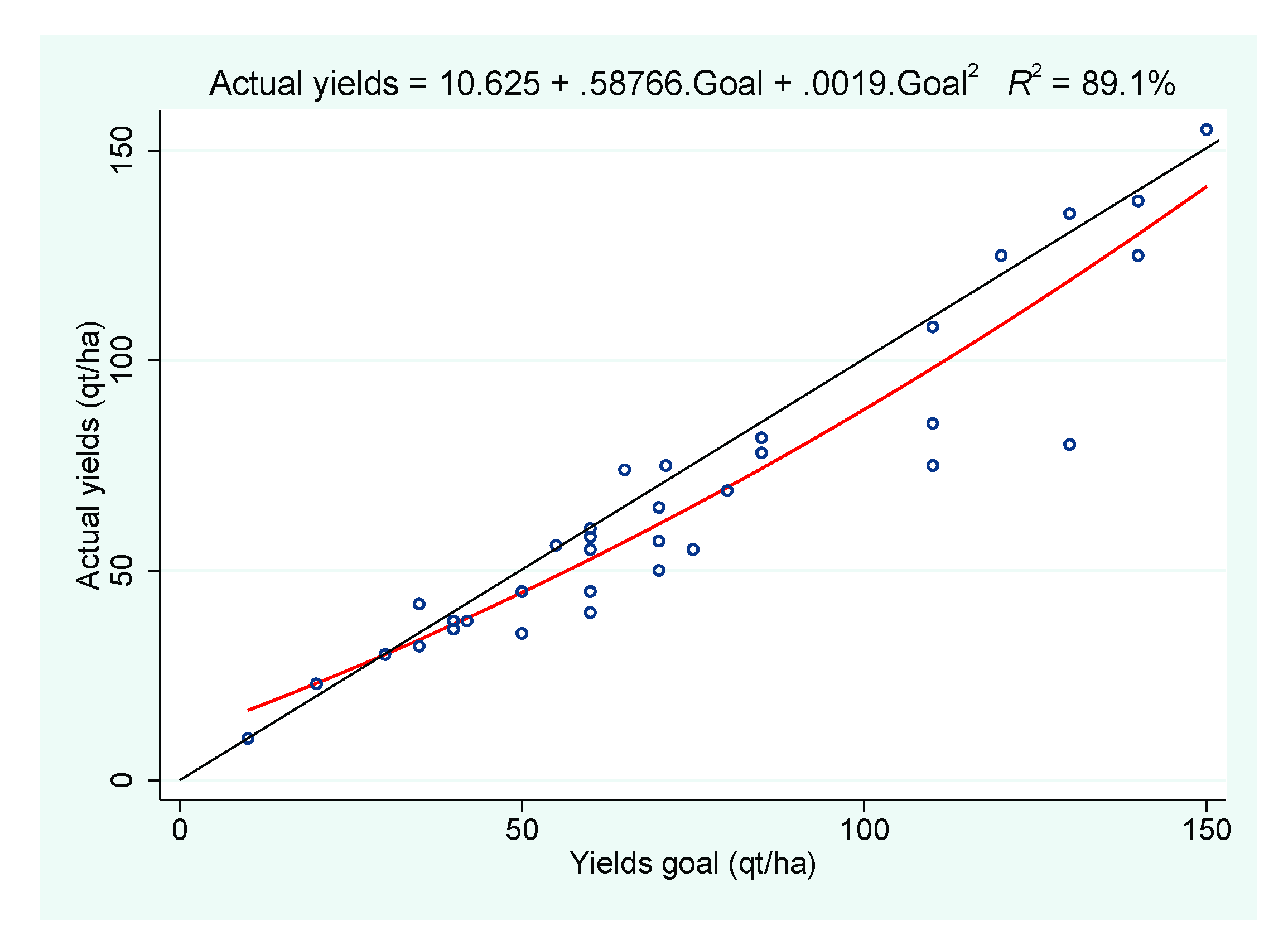
3.2.1. Crops and Yields

The sample consists of farmers whose main crops are cereals (75.72%), followed by oilseed (10%), and miscellaneous other crops (vineyards, chestnuts, etc.). In France, 2% of arable lands are planted with vineyards, 34.56% with cereals (including seed production), 1.1% with oilseeds, 0.73% with fruit trees, and 5.47% with annual forages (especially ensilage maize) [38]. Consequently, in the sample, the crop composition deviated from the national figures. However, a common point may be highlighted: cereals dominate. This difference with the national figures is directly associated with the accessible cooperatives. The BANCO report [2], which is at the origin of the MACC estimation, was focused on annual crops that are essentially represented by cereals in France. The work of Dequiedt and Servonnat [10] concerning risk and fertilization reduction only dealt with cereals and oilseed. In addition, the sample of farmers came from the same group of cooperatives (the benefit is based on the replication potential of the sample selection). The composition bias is, thus, limited to the fact that the perimeter of the abatement potential and cost estimation study corresponds in large part to these crops, and it does not apply to all the crops that can be found in France. However, it still has to be taken into account in the regressions if it leads to an estimation bias.
The descriptive statistics concerning yields for the main crops in the sample are presented: wheat (15 answers) and maize (7 answers). The average level of actual harvested yields for wheat is 61.16 qt/ha (std 15.12 qt/ha), and the average level of yield objectives is 67.16 qt/ha (std 14 qt/ha). The average level of actual harvested yields for maize is 118.7 qt/ha (std 35.5 qt/ha), and the average level of yield objectives is 123.43 qt/ha (std 30.24 qt/ha). The rate of difference between actual yields and objectives is −5% for wheat, and −4% for maize. Farmers are asked the reason for the difference according to their perception. They said that meteorological conditions were the main explanation, especially the quantity of rain that was too low or too high (71% of the cases for maize and wheat farmers).
Appendix D presents the relationship between actual yields and what was the objective at the beginning of the agricultural season. The results show that, in the sample the higher the goals are, the more difficult they are to achieve, with a better match for the highest goals. In addition, a rate of deviation is constructed in the form a c t u a l y i e l d s g o a l s g o a l s in order to observe the level of deviation on a normalized basis, which makes it possible to compare volumes. Results are presented in Appendix E. The average rate is −8.24% (std 0.14%, 37 answers). The average rate of yield objective achievement for crops is generally negative, strong for some crops (especially ensilage maize), and positive for two crops (maize seeds and sunflower).

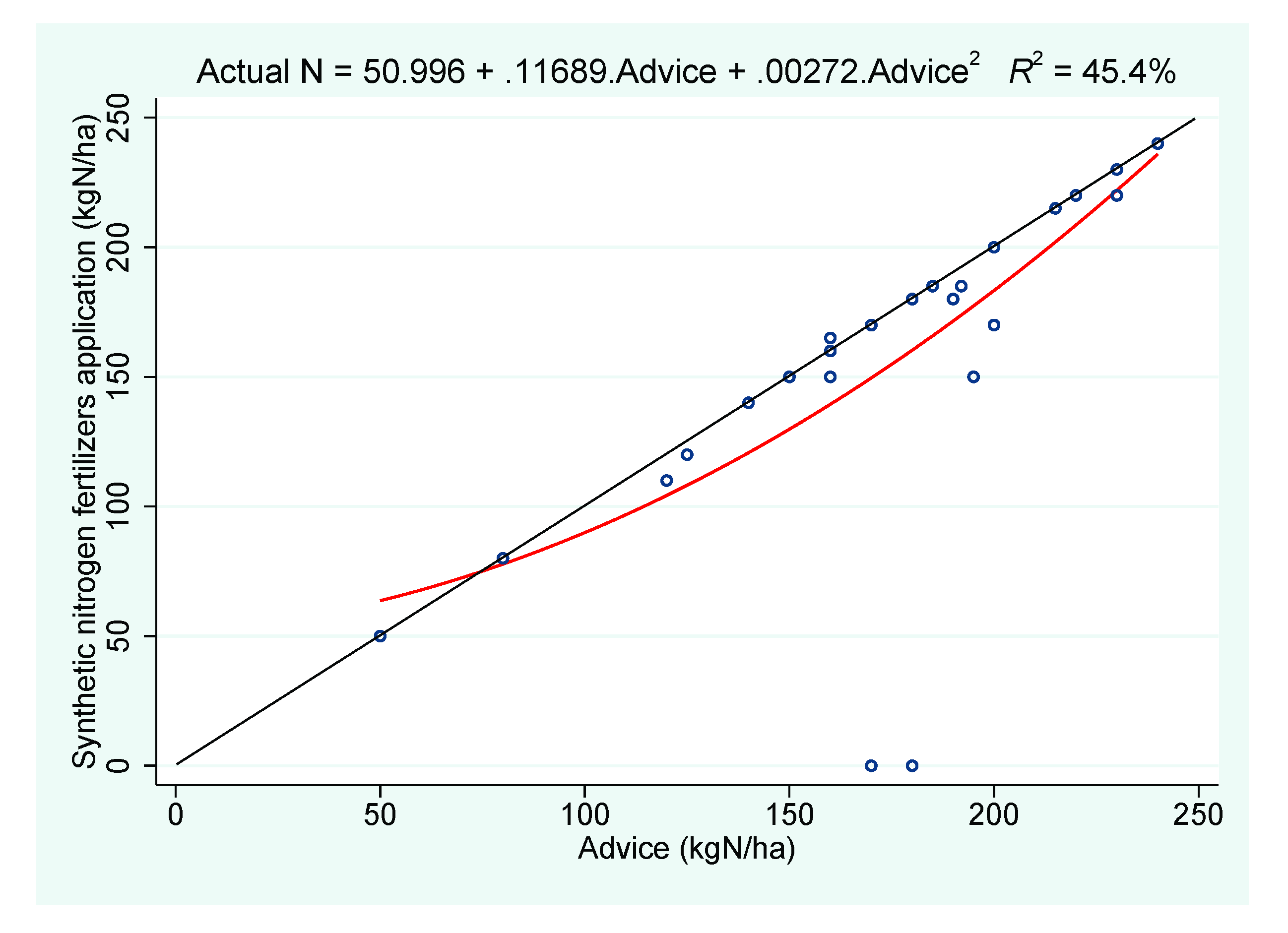
3.2.2. Synthetic Nitrogen Fertilization

A total of 95.6% of the respondents applied synthetic nitrogen fertilizers on their parcels. The share of operational costs associated with synthetic nitrogen fertilizer use on the declared parcels is 26% on average. This is important considering that, in general, labor (wage), mechanical soil work (fuel, etc.), seeds, other fertilizers, phytosanitary products, and potential irrigation might be contingent operational costs on the same parcel.
The nitrogen balance sheets give the total nitrogen fertilizer application on the parcel during the agricultural season (in kgN/ha). It does not make a lot of sense to observe the general statistics for this variable because it highly depends on the crop, and inter-crop comparisons are of no actual interest to the subject. The average level of fertilization is around 151 kgN/ha (std 72.5 kgN/ha, 37 answers), as indicated on Figure 1. This figure shows how farmers tend to follow recommendations from their cooperative agent in terms of fertilization for annual cropping. Farmers generally apply the recommended amount of fertilizers, except for some outliers. However, there are more deviations when the recommendations are higher.
Reducing the global synthetic nitrogen application balance sheet is an important mitigation practice. However, it relies on the actual nitrogen rates in the soils and depends on the alternative option in the event of an insufficient nitrogen rate. While alternatives (such as using legume crops in intermediary cropping) are not always applicable or efficient enough, another approach is to split the applications and to modulate each application in order to make the leaching by crops according to their needs over time more efficient, thus reducing the loss by non-absorption and the emission of N 2 O by volatilization. This is especially true for the first application at the beginning of the season (during the crop growth cycle) that can be a source of modulation, and advisers try to encourage farmers to apply less nitrogen fertilizers at the beginning of the season and, if necessary, to compensate with more fertilizer at the next application (side dressing). Moreover, the first application is associated with larger emissions [8]. Technically, the reduction of fertilization at the first splitting relies on the fact that nitrogen might still remain from the previous season and the prior crop if soils are correctly managed between seasons. In another vein, the first application is crucial and a source of uncertainty if poorly implemented: the beginning of the growth cycle is very important for the remainder of the campaign and for the yield goals (as well as quality goals) to be reached. Moreover, it may be impossible to apply side dressing in the advanced stages of the growing-blooming cycle depending on uncertain water access and field work conditions, so that risk-averse farmers would tend to apply more nitrogen than risk-neutral farmers at the first application [8,9,39]. However, the assumption that farmers associate clear and objective profit distribution with their fertilization practices is weak. This is because there may be more uncertainty about the future states-of-nature due to the embeddedness of several uncertain bio-physical factors in the prognostics related to side dressing possibilities. How splitting is implemented by the farmers in the sample is important to observe, and how it deviates from the recommendations of the cooperative agents in relation to farmers’ risk and ambiguity preferences is important, too. The average level of fertilization at the first application is around 50.5 kgN/ha (std 24.7 kgN/ha, 37 answers). Once again, it considerably depends on crops, and inter-crop comparisons are not within the scope of the current study. The same graph as in Figure 1 is computed for the first application of fertilizer. The results are presented in Appendix E, and the same kind of behaviors are observed.
Indicators were developed about the degree to which farmers tend to follow advice in terms of total synthetic nitrogen fertilizer application, fertilizer application for the first application, and the number of splitting. Farmers’ preferences under uncertainty may impact the willingness to follow advice, if the assumption of uncertainty associated with their consequences is valid. The two first indicators share the same structure: a c t u a l p r a c t i c e a d v i c e a d v i c e . They are a normalized rate of matching that is negative if farmers put less than recommended, positive if they put more, and null if they perfectly match the recommendations. The farther they go from 0, the more the farmer deviates from the recommendation. The average rate of matching for total fertilization is −0.08 (std 0.21, 33 answers), and it is −0.043 for the first application (std 0.28, 23 answers). For the number of splittings and related recommendations, which is a relative integer, the indicator is just the difference between the actual number and the recommended number. 0.5 means a semi-split: it is a situation where two different splittings were possible for the adviser (e.g., 2 or 3, or 4 or 5), and the farmer had the choice. The average difference between recommendations and actual practices is 0.1 (std 0.5, 29 answers). A total of 79% of the farmers applied exactly what they were told to do in terms of splitting.
Seventeen respondents were placed in a “vulnerable zone” for the questioned parcel, a specific recognition of environmental quality on the parcel and the risk in terms of ecological destruction if certain farming practices are used (approximately 37%, but there are many missing answers). This official zoning implies obligation and forbidden practices, especially in terms of nitrogen fertilization. In the sample, the average maximum authorized quantity of nitrogen fertilization is 154.6 kgN/ha (16 answers). A total of 20.6% declared having a mandatory fertilization method, such as using only organic fertilizer, a liquid product, or bovine manure (34 answers). These statistics give an idea of the weight of regulation on respondents, despite the regular lack of answers to these questions.

3.2.3. Other Practices and Characteristics

Farmers who applied organic fertilizer (e.g., manure) on the parcel were asked how they take the amount of nitrogen contained in this product into account. Among the 34 answers collected, only 35.56% used the reference table (very generalist in terms of information), only 20% used an analysis of the product (the most precise source of information), and 4.4% used both, while 15.56% did not take the amount of nitrogen into account. This application of organic-based nitrogen was taken into account for the synthetic nitrogen application by 90.32% of the respondents (31 answers). Thus, the precise level of nitrogen that is applied is not always known by farmers before they apply fertilizer on their parcels. Some 59.38% of farmers that applied organic fertilizer buried it through tillage (32 answers). Only 4.9% of farmers did not apply any nitrogen fertilizer. Some 56% applied both on their parcel, while 39% applied only synthetic fertilizer, and none of the farmers applied only organic fertilizers (41 answers).
Respondents were from the Drôme (31.71%), Meuse (21.95%), Tarn (21.95%), Charente-Maritime (12.20%), Isère (7.32%), and Meurthe-et-Moselle (4.88%) departments, revealing a wide geographic dispersion with a non-homogeneous composition. This presents the advantage of providing a control for some fixed local characteristics that can be captured through department of origin (or the town). The disadvantage is that crucial heterogeneous unobservable variables that diversely impacted the locations and that can explain individual farming choices cannot be controlled for. A total of 43.9% of the respondents own the parcel, and 66.1% are tenants. Approximately 36.59% of the farmers cropped their parcel under a contract that mainly concerned seed production, product quality, and industry-related sales. This characteristic can be important, especially in the case of quality contracts, because good quality in terms of product protein in some cases (especially for wheat) requires specific amounts of nitrogen (less than for the “quantity-focused” cases). Some 32.5% of the respondents held a crop insurance contract during the season (40 answers), which is close to the national level. The average size of the parcel was 15.34 ha. The average total area of the farms was 149.7 ha, which is more than twice the national average of approximately 58 ha in 2013, according to Eurostat. The composition in terms of crops, as well as location specificities and selection effects associated with the cooperative (InVivo group and its affiliations), may partly explain this difference. The average perceived CAP annual subsidy was €34,276 in the sample, and the average subsidy specifically related to environment was €3524 (10.3% of the total).

3.2.4. Socio-Demographic Statistics

The socio-demographic characteristics of the sample are presented in Appendix F. A total of 97.6% of the sample is composed by males (41 answers). The average age is 45.3 years old, ranging from 16 to 66 years of age. In France, the average age of male farmers is 49 years (53 years for females), and 61% of the farmers are aged between 40 and 60 years old [40]. According to the data, 82% of the respondents are between 40 and 60 years old. The sample is more concentrated in terms of age, which may be related to the fact that belonging to a cooperative and being motivated about meetings creates a selection of farmers. Some 45% of the respondents are married, 42.5% are single, 10% are in a Civil Solidarity Pact, and 2.5% are divorced (40 answers). In terms of education level, 77% of the respondents have a Baccalaureate (39 answers). At least 41% are Bac+2 and not beyond, which may correspond to an agricultural post-Bac technical diploma. A total of 23% dropped out of school after the Bac. Only 18% have a middle school certificate. In France, 17% of farmers went beyond the Baccalaureate, and 44% of French farmers dropped out after middle school [38]. This shows that the sample consists of farmers better educated than the general population of farmers at the country level. This is partly due to the composition in terms of age of the sample (32% are less than 40 years old, compared to 23% for France) because younger farmers have access to a better education than the former generations [38]. Some 41% of the households in the sample consist of at least four people, 30.8% consist of the farmer alone, and the remaining part is two or three people in the household (39 answers). The average number of people in the household is 1.652. A total of 52% of respondents have two children, 20% have no children, 12% have three children, and the rest have either one or more than three children (25 answers). The average number of children in the household is 1.88. The statistics concerning the farmers’ revenues show that 8.11% of farmers earn less than €1000/month, whereas 24.32% earn more than €3000.

3.3. Pairwise Correlations and Marginal Impact Estimations

3.3.1. Correlations

Pairwise correlation estimations (Pearson or Spearman) between all the measures of risk and ambiguity attitudes with interest variables were performed: the total level of nitrogen fertilization, the level of fertilization at the first application, the number of splittings in fertilizer applications, the difference between the total recommended application and what was actually applied, the difference between the actual and recommended first application, and the difference between the number of recommended and actual splittings. No significant correlations were found with the Pearson coefficient applied on continuous variables. The Pearson coefficient fails to estimate correlation coefficients for ordinal or categorical variables. The Spearman rank-order coefficient is suited to estimate correlation coefficients with categorical variables. Only one almost significant (p-value = 0.13) positive Spearman correlation was found between the NRC (ambiguity) and the level of fertilization at the first application (Spearman = 0.28). This would be the sign that farmer applies more nitrogen at the first fertilization splitting when they are ambiguity-averse. Bontems and Thomas [9] and Sheriff [8] show that side dressing nitrogen fertilization can be cost-efficient (better use of input) but depends on the propensity of farmers to take the risk that future natural conditions may prevent them from making other applications after the first splitting. A negative relationship was found between the categorical variable of risk aversion and the number of fertilization splittings, but the coefficient is not significant. The main result with the Spearman rank-order coefficient shows a new relationship: ambiguity aversion leads farmers who agreed to split applications to apply more at the first stage in a situation where they are totally uncertain about what the future conditions will be. This may be the sign that when the risk of splitting is taken, ambiguity aversion encourages farmers to hedge against the probabilistic uncertainty that they are exposed to. However, many other factors can explain this phenomenon and cannot be tested since ceteris paribus is not respected.

3.3.2. Taking Sampling Design in Regressions into Account

The observations in the sample were not individually selected: the experiment was performed randomly on the available farmers in regular meetings that took place in the cooperatives. However, the probability of being “selected” in the sample directly depended on the individual characteristics of the respondents (crop, soil, etc.) that led them to be part of these experiment groups and simultaneously impacted individuals’ decisions. These characteristics are heterogeneously repeated in the sample, so that the composition of the sample is not the same as for the total population. Any regression that would be run without correcting for these sampling selections would attribute false phenomena to the whole population of farmers, whereas the results would be only accurate for the sample at stake. Ignoring selection weight can, thus, lead to biases in estimation, and it is possible to fix this issue by attributing a probability weight to each observation. Finding the proper variables that can be used to make good sampling weights depends on the available data and on the assumption concerning the probability of selection. The crop that the farmers choose for their parcel appears to us to be a good weighting variable since the composition of the sample is widely determined by crops, and targeting cooperatives that work with annual non-perennial crops was one of the selection criteria. The composition bias can be important, since two main crops compose the sample and bear specific agronomic and economic characteristics (wheat and maize). Moreover, respondents generally responded well to this question. Adding probability weighting is feasible with Stata: the dependent and independent variables of each row are multiplied by a weight that corresponds to the opposite of the probability of having planted each crop on the parcel, and the variance-covariance matrix is estimated through a robust sandwich estimator. The more a crop represents a big proportion in the sample, the smallest the multiplied factor will be.
The observations were collected per group (local cooperatives), meaning that there may be correlations between error terms between observations within the same group, leading to a failure of the homoskedasticity assumption. These clustering can be taken into account in the regressions by applying adjustment weighting coefficients to subgroup standard error covariance matrices in order to correct heteroskedasticity. The local cooperative groups that the farmers belong to are assumed to be natural clusters among which respondents are concentrated, and some unobservable phenomena may uniformly affect the group. This subgroup captures correlation between behaviors, as well as a part of the exogenous natural hazards. A White [41] heteroskedasticity test may be used that is consistent with standard error estimation in order to fix for heteroskedasticity issues, but it does not allow clustered variability to be corrected, and the adjustment is at the individual level. Both will be compared.

3.3.3. Regressions Results

Twelve OLS regressions were carried out to try to explain the total fertilization and the fertilization at the first splitting. These regressions differ in several ways. They take weighting and/or clustering into account and they consider either the categorical variable (risk-loving/averse, ambiguity-loving/averse) or the number of safe (NSC) and risky (NRC) choice. Table 4 and Table 5 present the most robust regressions, i.e., considering weighting and clustering. Other results are presented in Appendix G. Only regression with significant coefficients are commented. Given the limited number of observations, most of the relevant regressions were the ones with at least 30 observations. This is the highest average number of observations obtained. Given the low number of degrees of freedom, the regressions are limited to one independent variable.
Table 4 shows that being in the risk-averse category leads to a significantly lower level of total fertilization compared to the reference category of risk-neutral farmers (coeff. = −48.84 significant at the 1% level). In contrast, Table 5 shows that being more ambiguity-averse (NRC) has a positive marginal impact on the quantity of nitrogen fertilizers applied at the first split (coeff. = 1.422 significant at the 10% level). These results have to be interpreted simultaneously.
The first one indicates a phenomenon that is consistent with numerous common assumptions about the positive impact of risk aversion on nitrogen fertilization. In the literature review, the role of risk aversion on fertilization is not clear-cut and depends on the risk-increasing or decreasing nature of the input (and, therefore, on the natural states-of-nature in terms of meteorological conditions and complementarity with water and pesticide uses). In the sample, nitrogen fertilizers do not appear to be considered as a risk-decreasing input. This lowers the assumption that risk aversion can be a barrier to the adoption of practices that reduce the total quantity of fertilizers used because it, instead, looks like a driver of reduction. However, it is notable that the risk aversion variable at stake is the categorical one: the reference category chosen for comparison is category 2, for risk neutrality. The coefficient is, therefore, the average level of fertilizers used by risk-averse farmers in general, compared to risk-neutral farmers in general.
The second result is the most original. Ambiguity aversion leads to using more fertilizers at the first application split (see Table 5), which is equivalent to saying that having an aversion for making bets on outcomes whose probabilistic distribution is uncertain encourages farmers to hedge against future possible nitrogen lacks. This result is interpreted as follows: if cooperative agents ask farmers to split their application, the first application is the most crucial, not only because it takes place at the beginning of the growing stage for the crop, but especially because the farmer does not know if it will be possible for her/him to fertilize again in the future because future states-of-nature are deeply uncertain. The possibility to make future splittings is dependent on this inability to make complete forecasts about entangled natural conditions. In order to extend more the interpretation to the lottery experiment, it is possible to say that the ambiguity-averse farmers insure themselves by applying more fertilizer at the first splitting, which is exactly what the cooperative agents do not want them to do because they prefer to bet on a risky practice rather than on an ambiguous one. However, this impact is much smaller than the negative impact of risk aversion on total fertilization. Moreover, splitting practices induce a dynamic evaluation of profits and optimal input uses, as shown in Bontems and Thomas [9], which implies other potential explanations, such as information value. This was not tested in this study. The benefit from splitting is, according to Bontems and Thomas [9], to allow the farmers to gather information about the true nitrogen needs of the crops and to be more efficient in their first and side dressing application, thus reducing production costs. This study shows that ambiguity aversion may impact the total benefits from information value and is a complementary driver of fertilization decisions.
The low number of observations for each regression (31) nuances the results. Adding control variables for crops (17 modalities), soil quality (21 modalities), previous crops (22 modalities), interactions between risk and ambiguity preferences, differences between actual yields and yield goals, and the perception of experienced risks at the last season by farmers, as well as several controls for agricultural practices and socio-economic and demographic variables, would produce more robust results and limit the biases that may be experienced. Because each modality of the categorical variables represents a covariate, the necessary number of observations would have to be significantly higher. Since the dependent variables related to fertilization are directly explained by obvious variables, such as the crop that has been planted on the parcel by the farmer or the soil quality, which is information asked in the questionnaire, it would be crucial to make the regression with these controls. This is an important limit of the econometric analysis.
The indicators about the degree to which farmers tend to follow advice in terms of total synthetic nitrogen fertilizer application, fertilizer application for the first application, and the number of splittings were not sufficiently matched with answers about risk and ambiguity preferences. This limits the number of observations that could be gathered and makes it impossible to make proper regressions with these variables.

4. Discussion

The respondents were found mostly risk-averse and ambiguity-neutral. This result is consistent with the conclusions of Barham et al. [30] for U.S. farmers and Chakravarty and Roy [22] for Indian students. The representativeness of the sample in terms of crops is low (when compared to French farmers) but is similar to previous studies about nitrogen fertilization reduction, which often test the same kind of crops: cereals and oilseeds [10]. The previous year was rather bad for the respondents since they generally fell short of their yield goals. The respondents did not fully follow what was recommended in terms of fertilization. In addition, many of them had to comply with fertilization regulatory rules on their parcel. They also considerably statistically differ from the national farmer population in terms of size of farm (bigger), age (younger), and education (more educated).
OLS regressions were performed with consideration of sampling design in order to produce the most robust estimations possible. Significant marginal impacts were found for only two dependent variables (when sample weights and clustering are introduced): the total quantity of nitrogen fertilizer used and the quantity of fertilizer used at the first splitting.
Being risk-averse is associated with a lower level of total fertilization (−48.8 kgN/ha on average) with respect to the reference category (risk neutrality). This result is not in accordance with the main conclusion in the literature [9,10,13,14,15]: risk aversion leads to an over-fertilization. Nevertheless, this result is interesting but difficult to analyze because it can be an indication that nitrogen fertilizers are perceived as being either risk-increasing or risk-decreasing (or neutral) by farmers, whereas the global levels of risk were perceived as being very low by farmers who self-insure with fertilizers. This could be an indication of diverse water and fertilizer use characteristics [39] and interactions between pest invasion risk with good growing conditions and crop growth level related to fertilizer use [42]. However, the total level of fertilization will always be associated with yield goals and the farmers’ agricultural knowledge for which they might have an objective probabilistic “mapping” and a clear ex ante stochastic production plan for the whole season.
The second main result is the positive marginal impact of ambiguity aversion (NRC variable) on the level of fertilization at the first splitting (+1.42 kg/ha for each higher level of risky choice). While this result seems to us unique, it echoes some previous research that highlighted the deep uncertainty that lay behind the splitting practice. For example, References [8,9] deal with the cost-effectiveness of side dressing fertilization. As future natural conditions are uncertain, the authors show that the farmer may not be able to perform other applications after the first splitting. Indeed, splitting fertilization is a good way to adapt fertilizer application to crop needs, but it relies on technical feasibility of postponed applications, which itself directly depends on unpredictable pedo-meteorological conditions and their deeply uncertain short-term fluctuations. Uncertain evolution of states-of-nature cannot be forecasted ex ante at the time of the first application, but the farmer may have subjective expectations and be more or less pessimistic about what can be expected. Within this scope, ambiguity aversion positively impacts the level of fertilization at the first application. However, the marginal impact is low, implying that even the global effect is negligible compared to the first result. The net total estimated impact of the preferences measured on the overall fertilization is negative. Moreover, the first result is significant because of sampling weight, while the second is significant because of clustered heteroskedastic-robust standard errors. The first case is not surprising, whereas the second one indicates that the significance of the result depends on the consideration of specific cluster-dependent unobservable variables, such as very local fluctuations and characteristics. This is interesting because it confirms the interpretation about the NRC result. Indeed, ambiguity associated with the first splitting is embedded in the individual deep uncertainty about the technical and natural feasibility of postponed splittings. This feasibility may be essentially local-specific and, consequently, partly shared by farmers from a given cooperative. In another vein, it is possible that the cluster-corrected standard errors account for unobserved impacts on group-variations that are directly related to the differences that could have occurred in the measurement processes between cooperatives. Even though the exact same experiment was reproduced on each farmer, there may have been slight differences that could have led to group-specific measurement errors (day, time of day, context, etc.), a phenomenon specific to field experiments compared to laboratory experiments.
Some limitations linked to internal and external validity may be identified. The estimations are limited by the number of respondents and the subsequent number of valid answers. This limits the external validity of the results. This experiment may be seen as a pilot for a wider experiment, and allows us to observe if the current results are robust or not to all the necessary controls. In terms of internal validity, it would be interesting to test for the impact of time preferences in a subsequent study. Time preferences explain choices at each step of production, as well as decisions in terms of practices and production goals. Secondly, the use of the MPL procedure entails advantages and disadvantages. The specific versions of the lotteries used rely on calibrations associated with the widely accepted assumption of a CRRA (power) utility function, and its form (chained lotteries with switching points) allows for the precise measurement of the level of risk aversion on the continuous distribution of gains. Moreover, its wide use in the literature makes it possible for us to effectively compare the results. The main problem is to identify the actual preferences of the respondent. First, if the preferences of the agent do not follow a CRRA utility function or, more generally, if the individual has preferences that are not in line with the expected utility framework, then the method is not relevant. This would lead to the risk that the subsequent regressions would have a limited internal invalidity and, consequently, limited results. Second, as mentioned in the literature review, some criticisms have been put forward by Drichoutis and Lusk [43]. However, these disadvantages did not prevent several studies from producing credible results (see literature review in the introduction).

5. Conclusions

An experiment on farmers was implemented in partnership with their cooperative group (InVivo) in order to test the main assumption using real data: uncertainty may be a barrier to nitrogen fertilization reduction. Two levels of preferences toward uncertainty were tested: risk attitudes (known probability) and ambiguity attitudes (unknown probability). The goal was to estimate the interactions between those measures and the mitigation potential associated with fertilizer reduction. The role of these individual behavioral attitudes was tested in terms of different practices related to fertilization, fertilization practices per se (global level of fertilizer, level of fertilization at the first splitting, number of splittings), and farmers’ willingness to follow recommendations from their cooperative agents who encourage them to adopt more environmentally-friendly practices. The role of several agricultural, regulatory, and socio-economic characteristics was also tested, as well as their preferences, embedded with uncertainty, on fertilization practices and the propensity to follow recommendations. The results show that, in the sample, French farmers are mostly risk-averse and ambiguity-neutral. The major conclusion is the following one: risk aversion reduces the global level of fertilization, whereas ambiguity aversion increases the level of fertilization, at the first application.
These results have several implications in terms of public policies. First, this study shows that risk and ambiguity attitudes impact abatement costs associated with nitrogen fertilization reduction to some degree. While ambiguity aversion is a hidden cost of innovative fertilization practices, such as splitting, risk aversion can be a “hidden abatement benefit” for global reduction of nitrogen application. These phenomena question then the optimality of flat rate subsidies. Fluctuations in production conditions can cause the abatement costs to fluctuate mechanically, and subsidies aimed at offsetting potential losses from reduction can become a windfall for farmers, the majority of whom would adjust their use of fertilizer by themselves. This leads us to question the usual recommendations when considering risks, such as subsidized crop insurance that would cover yield risk and, in this way, encourage farmers to lower their fertilization rate. Since this depends on the interaction between nitrogen fertilizers and the environment in which they are applied, as well as the crop, it can even have counter-productive effects on N 2 O mitigation. The literature shows that fertilization splitting has a huge benefit in terms of information value. This explains why farmers would not be so reluctant to adopt this practice. However, if ambiguity aversion increases the level of application at the first splitting and, therefore, increases emissions, it could be good to instead reduce uncertainty through generalized soil testing in order to secure information while developing new methods to ensure that side dressing will be possible later in the season. Other varied types of options can also be proposed to improve farmers’ knowledge about the reaction of crops to these new forms of nitrogen management over the growing period. In addition, 8.5% of the French farming surface area is now certified organic, with some 47,000 farms. Given the ambitious objectives of the Ambition Bio 2022 plan to convert 15% of the farmed agricultural surface area to organic farming by 2022 and increase organic food consumption in the country, it seems relevant to question the multiple private costs that can prevent farmers from entirely eliminating nitrogen inputs. Indeed, the transition from conventional to organic farming means that farmers are willing to operate under uncertain conditions and to rely far more on the interactions between crops and their environment. The paper shows that considerations, such as ambiguity aversion and related costs (information, testing, and trials), would allow farmers to modify their production habits more rapidly than with only classic compensation subsidies.
Several future research directions may be considered in relation with the limitations evoked at the end of the discussion. First, the measurement of the time preferences, in addition to the preferences towards risk and ambiguity, may be an interesting direction. Second, some papers [21,23,44] demonstrate that farmers, among them the French ones, do not conform with the expected utility framework and that they rather align their behaviors with Prospect Theory [45]. Consequently, it may be interesting to suppose such a new framework and to use the Multiple Price List method proposed by Tanaka et al. [44] to elicit the different parameters of the utility function. This approach will allow us to go one step further by considering loss aversion, too.

Author Contributions

Both authors designed the questionnaire and collected the answers in the field. C.T. was responsible for the data analysis and wrote the first draft of the article. M.B. supervised the work of C.T., read and commented on the different versions of the article. M.B. realized the revisions required by the reviewers. Both authors have read and agreed to the published version of the manuscript.

Funding

This research received no external funding.

Institutional Review Board Statement

Not applicable.

Informed Consent Statement

Informed consent was obtained from all subjects involved in the study.

Data Availability Statement

Not applicable.

Acknowledgments

This work is part of the Agriculture and Forestry research program of the Climate Economics Chair. The authors would like to thank the Climate Economics Chair for their financial support. The authors are also very grateful to AgroSolutions (InVivo group) for their support of this work. The UMR BETA is supported by a grant overseen by the French National Research Agency (ANR) as part of the “Investissements d’Avenir” program (ANR-11-LABX-0002-01, Lab of Excellence ARBRE). Finally, the authors gratefully acknowledge the editors and the anonymous reviewers for their valuable comments.

Conflicts of Interest

The authors declare no conflict of interest.

Appendix A. Survey on the Use of Synthetic Nitrogen Fertilizers

The survey you are going to participate in aims at studying the climate change mitigation measures of the French agricultural sector. In particular, the survey focuses on farmers’ fertilization decisions. Nitrogen fertilization is one of the main greenhouse gas emissions in the agricultural sector. The aim is to improve the understanding and determinants of fertilization decisions, particularly by focusing on an economic parameter that reflects individual preferences for risky choices.
This survey is conducted as part of a joint project between the INRAE (National Research Institute for Agriculture, Food, and the Environment), the Climate Economics Chair (CEC), and InVivo. More specifically, this work is part of a thesis in economics, conducted within INRAE.
The questionnaire will consist of three parts. In the first part, it will be necessary to make hypothetical choices between two options. These choices will help measure your individual attitude towards risk. This method is widely used in economics to reveal to individuals their preferences for more or less risky situations. The second part will be composed of questions relating to your management decisions and, more particularly, fertilization. The final part of the survey will focus on your socio-economic characteristics.
There are no good or bad answers during the survey, just different behaviors to observe. For the purposes of the survey, you must answer all the questions. The confidentiality of the information contained in this questionnaire is ensured by the anonymity of the respondent. Your answers will remain confidential. The results will be presented in synthetic form in scientific publications with scrupulous respect for the anonymity of the respondents. Once the data is processed, it will be returned to you individually and you can compare your results to the average of our sample and your cooperative.
The lack of communication between participants is a guarantee of success. We ask you not to discuss with other participants during the survey.
Part 1: Choice between Two Options
This first part is composed of two series of 10 decisions represented by two tables.
All questions correspond to fictitious situations for which we ask you to answer as if you were facing a real situation, taking the necessary time to choose the answers that best correspond to your preferences.
First table:
For each of the 10 decisions (lines), you must choose which of the two options (A or B) you prefer. Let’s take an example. Decision 1 of the table reads as follows:
-
Option A: obtain €7 with 10% chance or €5 with 90% chance.
-
Option B: obtain €13 with 10% chance or €0 with 90% chance.
Decision 1 can also be represented in the form of a circular graph:
Sustainability 13 09802 i001
The following decisions read in the same way; only the probabilities associated with earnings change. Please complete the boxes below the table.
DecisionsOption AOption B
Proba.PayoffProba.PayoffProba.PayoffProba.Payoff
110%€790%€510%€1390%€0
220%€780%€520%€1380%€0
330%€770%€530%€1370%€0
440%€760%€540%€1360%€0
550%€750%€550%€1350%€0
660%€740%€560%€1340%€0
770%€730%€570%€1330%€0
880%€720%€580%€1320%€0
990%€710%€590%€1310%€0
10100%€70%€5100%€130%€0
-
I choose option A for decisions 1 to □.
You can answer with a number between 1 and 10. If you choose 3, it implies that option A is chosen for the first three lines, then B for the following ones. If you choose 1, it implies that you choose A only for the first line, and B for the others. If you do not choose anything, it implies that you choose B for all lines: you will have to answer 1 in the next question.
-
I choose option B for decisions □ at 10.
Second table:
For each of the 10 decisions (lines), you must choose which of the two options (A or B) you prefer. This time, both options are likened to a draw in an urn composed of 10 balls of black or white colors. Option A corresponds to an urn composed of 5 black balls and 5 white balls. If you choose this option, you know that you have 5 chances out of 10 (or 1 chance out of 2) to win. In other words, the probability of winning is equal to 50%.
Option B corresponds to an urn whose exact composition is not known. If you choose this option you do not exactly know your chance to win. This varies between 0 chance out of 10 (for example, you choose the white ball, and the urn contains only black balls) and 10 chances out of 10 (for example, you choose the white ball and the urn contain only white balls). In other words, the probability of winning is between 0% and 100%.
Prior to the 10 decisions, you will have to choose the color that you consider as winning, black or white.
Choose a color: BLACK □ or WHITE □
Let’s take an example. Decision 1 of the table reads as follows:
-
Option A: obtain €13 with 1 chance out of 2 (50%) or €0 with 1 chance out of 2 (50%).
-
Option B: obtain €9 or €0, but you do not know the associated chances of winning.
Decision 1 can also be represented in the form of an urn as illustrated below:
Sustainability 13 09802 i002
The following decisions read in the same way, only the potential gains for Option A change. Please complete the boxes below the table.
DecisionsOption A: urn AOption B: urn B
In urn A, the Distribution ofIn urn B, the Distribution
BALLS Is 5 Black and 5 Whiteof Balls Is Not Known
Chosen ColorChosen ColorChosen ColorChosen Color
ObtainedNot ObtainedObtainedNotObtained
1€13€0€9€0
2€12€0€9€0
3€11€0€9€0
4€10€0€9€0
5€9€0€9€0
6€8€0€9€0
7€7€0€9€0
8€6€0€9€0
9€4€0€9€0
10€2€0€9€0
-
I choose option A for decisions 1 to □.
You can answer with a number between 1 and 10. If you choose 3, it implies that option A is chosen for the first three lines, then B for the following ones. If you choose 1, it implies that you choose A only for the first line, and B for the others. If you do not choose anything, it implies that you choose B for all lines: you will have to answer 1 in the next question.
-
I choose option B for decisions □ at 10.
Part 2: Management decisions on the largest plot of your farm, excluding pasture
We wish to remind you that all the answers to this questionnaire will be totally anonymous and will not be treated in any way outside the scientific publication for which they are intended.
For this part of the questionnaire, we will refer to the largest plot of your farm, excluding pasture. We would like to know more about your farming practices on this plot during the last crop year.
  • Location:
    Which department?
    On which commune is your parcel located?
  • What is your status vis-à-vis the parcel in question? □ Owner □ Tenant
  • What is the main crop?
  • Is it a contract crop? □ No □ Yes
    If yes, what kind of contract?
  • What is the smallest area on the plot (in hectares)?
  • What is the type of previous crop on the plot?
  • What is the type of soil on the plot?
  • What was your target for early returns (in qt/ha)?
  • What were your real yields after harvest (in qt/ha)?
    If objective and real returns were different, please explain why:
  • Have you applied one (or more) organic nitrogen fertilizers on this plot? □ No □ Yes
    If yes, how much (in kg/ha)?
    How was the amount of nitrogen contained in this (these) input (s) taken into account? □ Analysis □ Reference table □ It was not taken into account
    Do mineral nitrogen fertilizer recommendations take this quantity into account? □ No □ Yes
  • Did you bury the fertilizer? □ No □ Yes
In terms of mineral nitrogen fertilization:
  • Please indicate the amount of mineral nitrogen recommended by your nitrogen advisory agency on this plot (in kgN/ha)?
  • Were there any recommendations on the first nitrogen input? □ No □ Yes
    If yes, how much (in kg/ha)?
  • Have you been advised to split contributions? □ No □ Yes
    If yes, how much?
  • Did you split the contributions? □ No □ Yes
    If yes, how much?
Regulatory Doses:
  • Is there a maximum that you should not exceed on this parcel? □ No □ Yes.
    If yes, how much (in kg/ha)?
  • Is there a type of spreading method that you must follow? □ No □ Yes
    If yes, which one?
    If yes, what is this regulatory constraint related to? □ Vulnerable area □ MAE □ Other
Actual decisions of mineral nitrogen fertilization:
  • How much did you actually apply to this parcel in total (in kgN/ha)?
  • And at the first intake (in kgN/ha)?
    Explain the reasons for your choice:
  • What is the share of synthetic nitrogen fertilizer costs in your total expenses for this parcel (in %)?
Some additional questions about your farm:
  • How much PAC assistance do you receive in total (in €/year)?
    Of this total amount, how much corresponds to specific environmental aids and reduction of the chemical spreading (MAE or other) (in €/year)?
  • Have you taken out a voluntary agricultural yield insurance contract this year?
    □ No □ Yes
  • What is the total area of your farm (in hectares)?
  • Are you part of an operator’s union? □ No □ Yes
    If yes, which one?
Part 3: Socio-economic characteristics
Answers to these questions are essential to properly analyze your decisions. We remind you that your answers will be treated anonymously.
  • What is your age in years ?
  • Sex: □ Man □ Woman
  • Marital status: □ Single □ Married □ Civil Solidarity Pact
  • Level of studies:
    □ Without diploma □ Brevet □ Bac
    □ Baccalaureate + (specify the number of years of study after the Baccalaureate: …)
  • Number of people in the household: □ 1 □ 2 □ 3 □ 4 and more Among them, how much children ?
  • In what interval are the total monthly incomes of your household (net of taxes)?
    □<€1000/net/month □ from 1000 to €1500/net/month
    □ from 1500 to €2000/net/month □ from 2000 to €2500/net/month
    □ from 2500 to €3000/net/month □> €3000/net/month
  • Please express your opinion of synthetic nitrogen fertilizers and policies to regulate their use:
  • Please give us your opinion of the survey (strengths, possible difficulties encountered, etc.):
Email address for the return of the results:
Thanks for your help; we will transmit your individual results after they are processed.

Appendix B. The Ten-Paired Lottery Choice

Table A1. The ten-paired lottery choice decisions under risk.
DecisionsOption AOption B
Proba.PayoffProba.PayoffProba.PayoffProba.Payoff
110%€790%€510%€1390%€0
220%€780%€520%€1380%€0
330%€770%€530%€1370%€0
440%€760%€540%€1360%€0
550%€750%€550%€1350%€0
660%€740%€560%€1340%€0
770%€730%€570%€1330%€0
880%€720%€580%€1320%€0
990%€710%€590%€1310%€0
10100%€70%€5100%€130%€0
Table A2. The ten-paired lottery choice decisions under ambiguity.
DecisionsOption A: urn AOption B: urn B
In urn A, the Distribution ofIn urn B, the Distribution
Balls Is 5 Black and 5 Whiteof Balls Is Not Known
Chosen ColorChosen ColorChosen ColorChosen Color
ObtainedNot ObtainedObtainedNot Obtained
1€13€0€9€0
2€12€0€9€0
3€11€0€9€0
4€10€0€9€0
5€9€0€9€0
6€8€0€9€0
7€7€0€9€0
8€6€0€9€0
9€4€0€9€0
10€2€0€9€0

Appendix C. Pairwise Pearson Correlations Estimations

In order to reinforce the conclusions about correlation between risk and ambiguity measures, pairwise Pearson correlations estimations were proposed. Three variables of preferences were linked: the categorical variable, the initial variable of NSC and NRC, and the coefficients associated with the midpoint of each class. The associated results are presented in Table A3.
Table A3. Pearson correlation coefficients (* p < 0.1).
Categ.Categ.MidpointMidpointNSCNRC
(Risk)(amb.)(Risk)(amb.)
Categ. (risk)1.000
Categ. (amb)0.2361.000
Midpoint (risk)0.679 *0.0471.000
Midpoint (amb.)−0.753 *−0.033−0.989 *1.000
NSC0.711 *0.0480.977 *−0.989 *1.000
NRC0.1000.851 *0.089−0.0850.1341.000
The positive significant correlations in the case of risk are not surprising because they always correspond to variables that covariate by construction. The interesting thing to note is the significant and strong negative correlation between the midpoint variable for ambiguity and all the variables related to risk. Since the coefficient of ambiguity aversion is a descending variable, this result shows that more risk aversion is correlated with more ambiguity aversion. This result is in line with previous ones indicating a significant and positive correlation between risk and ambiguity preferences [22,46,47].

Appendix D. Additional Results for Crops and Yields

Figure A1 plots the relationship between actual yields and what was the objective at the beginning of the agricultural season. The bisectrix (dark line) shows a hypothetical situation where there would be a perfect match between the ex ante objective and the actual level of yields. A positive and slightly convex relationship between both (red line) may be observed, which is a sign that, in the sample, the higher the goals are, the more difficult they are to achieve, with a better match for the highest goals.
Figure A1. Relationship between actual and objective yields. Red curve is the quadratic relationship between y and x; dark line is the bisectrix.
Sustainability 13 09802 g0a1
A rate of deviation was constructed in the form a c t u a l y i e l d s g o a l s g o a l s that makes it possible to compare volumes. Results are presented in Figure A2. The average rate is −8.24% (std 0.14%, 37 answers). The average rate of yield objective achievement for crops is generally negative, strong for some crops (especially ensilage maize), and positive for two crops (maize seeds and sunflower).
Figure A2. Deviation rate between actual and objective yields.
Sustainability 13 09802 g0a2

Appendix E. Additional Results for Synthetic Nitrogen Fertilization

Figure A3. Relationship between actual and recommended first applications. Red curve is the quadratic relationship between y and x; dark line is the bisectrix.
Sustainability 13 09802 g0a3

Appendix F. Socio-Demographic Characteristics

Table A4. Socio-demographic characteristics.
Variables% of Respondents
Gender
Male97.6%
Marital status
Divorced2.5%
Married45%
PACS10%
Single42.5%
Education level
Middle school certificate17.95%
Agricultural school certificate2.56%
Agricultural technic diploma2.56%
Bac23.08%
Bac +241.03%
Bac +37.69%
Bac +42.56%
Bac +52.56%
Revenue ranges (/month)
<10008.11%
[1000, 1500[24.32%
[1500, 2000[10.81%
[2000, 2500[21.62%
[2500, 3000[10.81%
>300024.32%
Average age (year)
45.3
Average number of people in the household
1.652
Average number of children
1.88

Appendix G. Additional Results for the Regressions

Table A5. Total fertilization.
VARIABLES
Risk-loving−28.25 50.60
(54.07)(41.58)
Risk-averse−58.16−48.84 **
(41.43)(19.57)
Ambiguity-loving −12.2518.80
(32.17)(28.91)
Ambiguity-averse −30.70−14.52
(37.48)(40.08)
NSC 3.7546.827
(6.278)(4.775)
NRC −3.424−6.235
(6.794)(6.461)
Constant191.2 ***186.9 ***157.4 ***142.4 ***122.7 ***103.5 ***162.6 ***177.0 ***
(38.24)(8.863)(22.75)(25.72)(39.03)(34.51)(36.34)(33.83)
Weighting (crop)NoYesNoYesNoYesNoYes
Clustering (cooperative)NoNoNoNoNoNoNoNo
Observations3131313131313131
R-squared0.0740.0470.0230.0310.0120.0420.0090.030
F1.1213.5950.3360.6100.3572.0450.2540.931
p-Fisher0.3400.04080.7170.5500.5550.1630.6180.342
Standard errors in parentheses; *** p < 0.01, ** p < 0.05.
Table A6. Fertilization at the first splitting.
VARIABLES
Risk-loving1.7501.825
(19.35)(6.614)
Risk-averse 0.207 −4.310
(14.82)(6.873)
Ambiguity-loving 3.667 6.471
(8.682)(8.172)
Ambiguity-averse 3.7624.886
(10.11)(12.61)
NSC 0.7321.529
(2.171)(1.567)
NRC 2.0941.422
(1.796)(2.005)
Constant51.2 5 ***53.14 ***48.67 ***45.44 ***47.07 ***41.02 ***37.76 ***41.08 ***
(13.68)(3.747)(6.139)(6.655)(13.50)(10.77)(9.606)(10.03)
Weighting (crop)NoYesNoYesNoYesNoYes
Clustering (cooperative)NoNoNoNoNoNoNoNo
Observations3131313131313131
R-squared0.0010.0090.0190.0190.0040.0200.0450.018
F0.008730.3180.2770.3150.1140.9531.3600.503
p-Fisher0.9910.7300.7600.7320.7380.3370.2530.484
Standard errors in parentheses; *** p < 0.01.

References

  1. CITEPA. Inventaire SECTEN; CITEPA: Paris, France, 2019. [Google Scholar]
  2. Pellerin, S.; Bamière, L.; Angers, D.; Béline, F.; Benoit, M.; Butault, J.; Chenu, C.; Colnenne-David, C.; de Cara, S.; Delame, N.; et al. Quelle Contribution de L’agriculture Française à la Réduction des émissions de gaz à Effet de Serre? Potentiel d’atténuation et coût de dix Actions Techniques; Technical Report hal-01186943; INRA: Paris, France, 2013. [Google Scholar]
  3. Pope, R.; Kramer, R. Production uncertainty and factor demands for the competitive firm. South. Econ. J. 1979, 46, 489–502. [Google Scholar] [CrossRef] [Green Version]
  4. Moschini, G.; Hennessy, D. Uncertainty, risk aversion, and risk management for agricultural producers. In Handbook of Agricultural Economics, 1st ed.; Gardner, B.L., Rausser, G.C., Eds.; Elsevier: Amsterdam, The Netherlands, 2001; Volume 1, pp. 88–153. [Google Scholar]
  5. Roosen, J.; Hennessy, D. Tests for the role of risk aversion on input use. Am. J. Agric. Econ. 2003, 85, 30–43. [Google Scholar] [CrossRef] [Green Version]
  6. Leathers, H.; Quiggin, J. Interactions between agricultural and resource policy: The Importance of attitudes toward risk. Am. J. Agric. Econ. 1991, 73, 757–764. [Google Scholar] [CrossRef]
  7. Stuart, D.; Schewe, R.; McDermott, M. Reducing nitrogen fertilizer application as a climate change mitigation strategy: Understanding farmer decision-making and potential barriers to change in the US. Land Use Policy 2014, 36, 210–218. [Google Scholar] [CrossRef]
  8. Sheriff, G. Efficient waste? Why farmers over-apply nutrients and the implications for policy design. Appl. Econ. Perspect. Policy 2005, 27, 542–557. [Google Scholar] [CrossRef]
  9. Bontems, P.; Thomas, A. Information value and risk premium in agricultural production: The case of split nitrogen application for corn. Am. J. Agric. Econ. 2000, 82, 59–70. [Google Scholar] [CrossRef]
  10. Dequiedt, B.; Servonnat, E. Risk as a Limit or an Opportunity to Mitigate GHG Emissions? The Case of Fertilisation in Agriculture; Working Papers 1606; Chaire Economie du Climat: Paris, France, 2016; pp. 1–48. [Google Scholar]
  11. Gandorfer, M.; Pannell, D.; Meyer-Aurich, A. Analyzing the effects of risk and uncertainty on optimal tillage and nitrogen fertilizer intensity for field crops in Germany. Agric. Syst. 2011, 104, 615–622. [Google Scholar] [CrossRef]
  12. Monjardino, M.; McBeath, T.; Ouzman, J.; Llewellyn, R.; Jones, B. Farmer risk-aversion limits closure of yield and profit gaps: A study of nitrogen management in the southern Australian wheatbelt. Agric. Syst. 2015, 137, 108–118. [Google Scholar] [CrossRef]
  13. Meyer-Aurich, A.; Karatay, Y.N. Effects of uncertainty and farmer’s risk aversion on optimal N fertilizer supply in wheat production in Germany. Agric. Syst. 2019, 173, 130–139. [Google Scholar] [CrossRef]
  14. Meyer-Aurich, A.; Karatay, Y.N.; Nausediene, A.; Kirschke, D. Effectivity and cost-efficiency of a tax on nitrogen fertilizer to reduce GHG emissions from agriculture. Atmosphere 2020, 11, 607. [Google Scholar] [CrossRef]
  15. Wu, H.; Hao, H.; Lei, H.; Ge, Y.; Shi, H.; Song, Y. Farm size, risk aversion and overuse of fertilizer: The heterogeneity of large-scale and small-scale wheat farmers in Northern China. Land 2021, 10, 111. [Google Scholar] [CrossRef]
  16. Qiao, F.; Huang, J. Farmer’s risk preference and fertilizer use. J. Integr. Agric. 2021, 20, 1987–1995. [Google Scholar] [CrossRef]
  17. Binswanger, H. Attitudes toward risk: Experimental measurement in rural India. Am. J. Agric. Econ. 1980, 62, 395–407. [Google Scholar] [CrossRef] [Green Version]
  18. Eckel, C.; Grossman, P. Forecasting risk attitudes: An experimental study using actual and forecast gamble choices. J. Econ. Behav. Organ. 2008, 68, 1–7. [Google Scholar] [CrossRef]
  19. Holt, C.; Laury, S. Risk aversion and incentive effects. Am. Econ. Rev. 2002, 92, 1644–1655. [Google Scholar] [CrossRef] [Green Version]
  20. Reynaud, A.; Couture, S. Stability of risk preference measures: Results from a field experiment on French farmers. Theory Decis. 2012, 73, 203–221. [Google Scholar] [CrossRef] [Green Version]
  21. Bocquého, G.; Jacquet, F.; Reynaud, A. Expected utility or prospect theory maximisers? Assessing farmers’ risk behaviour from field-experiment data. Eur. Rev. Agric. Econ. 2014, 41, 135–172. [Google Scholar] [CrossRef]
  22. Chakravarty, S.; Roy, J. Recursive expected utility and the separation of attitudes towards risk and ambiguity: An experimental study. Theory Decis. 2009, 66, 199–228. [Google Scholar] [CrossRef]
  23. Bougherara, D.; Gassmann, X.; Piet, L.; Reynaud, A. Structural estimation of farmers’ risk and ambiguity preferences: A field experiment. Eur. Rev. Agric. Econ. 2017, 44, 782–808. [Google Scholar] [CrossRef]
  24. Akay, A.; Martinsson, P.; Medhin, H.; Trautmann, S. Attitudes toward uncertainty among the poor: An experiment in rural Ethiopia. Theory Decis. 2012, 73, 453–464. [Google Scholar] [CrossRef] [Green Version]
  25. Ghadim, A.; Pannell, D.; Burton, M. Risk, uncertainty, and learning in adoption of a crop innovation. Agric. Econ. 2005, 33, 1–9. [Google Scholar] [CrossRef]
  26. Cotty, T.L.; d’Hôtel, E.M.; Soubeyran, R.; Subervie, J. Linking risk aversion, time preference and fertiliser use in Burkina Faso. J. Dev. Stud. 2018, 54, 1991–2006. [Google Scholar] [CrossRef]
  27. Hellerstein, D.; Higgins, N.; Horowitz, J. The predictive power of risk preference measures for farming decisions. Eur. Rev. Agric. Econ. 2013, 40, 807–833. [Google Scholar] [CrossRef]
  28. Liu, E. Time to change what to sow: Risk preferences and technology adoption decisions of cotton farmers in China. Rev. Econ. Stat. 2013, 95, 1386–1403. [Google Scholar] [CrossRef] [Green Version]
  29. Engle-Warnick, J.; Escobal, J.; Laszlo, S. Ambiguity Aversion as a Predictor of Technology Choice: Experimental Evidence from Peru; Scientific Publications 2007s-01; CIRANO: Montreal, QC, Canada, 2007; pp. 1–41. [Google Scholar]
  30. Barham, B.; Chavas, J.; Fitz, D.; Salas, V.; Schechter, L. The roles of risk and ambiguity in technology adoption. J. Econ. Behav. Organ. 2014, 97, 204–218. [Google Scholar] [CrossRef]
  31. Brunette, M.; Cabantous, L.; Couture, S.; Stenger, A. The impact of governmental assistance on insurance demand under ambiguity: A theoretical model and an experimental test. Theory Decis. 2013, 75, 153–174. [Google Scholar] [CrossRef]
  32. Klibanoff, P.; Marinaci, M.; Mukerji, S. A smooth model of decision making under ambiguity. Econometrica 2005, 73, 1849–1892. [Google Scholar] [CrossRef] [Green Version]
  33. Beattie, J.; Loomes, G. The impact of incentives upon risky choice experiments. J. Risk Uncertain. 1997, 14, 155–168. [Google Scholar] [CrossRef]
  34. Camerer, C.; Hogarth, R. The effects of financial incentives in experiments: A review and capital-labor-production framework. J. Risk Uncertain. 1999, 1, 7–42. [Google Scholar] [CrossRef]
  35. Battalio, R.; Kagel, J.; Jiranyakul, K. Testing between alternative models of choice under uncertainty: Some initial results. J. Risk Uncertain. 1990, 3, 25–50. [Google Scholar] [CrossRef]
  36. Wik, M.; Kebede, T.; Bergland, O.; Holden, S. On the measurement of risk aversion from experimental data. Appl. Econ. 2004, 36, 2443–2451. [Google Scholar] [CrossRef]
  37. Dohmen, T.; Falk, A.; Huffman, D.; Sunde, U.; Schupp, J.; Wagner, G. Individual risk attitudes: Measurement, determinants, and behavioral consequences. J. Eur. Econ. Assoc. 2011, 9, 522–550. [Google Scholar] [CrossRef] [Green Version]
  38. Ministère de l’Agriculture et de l’Alimentation (MAA). Agreste, La Statistique, l’Evaluation et la Prospective Agricole; MAA: Paris, France, 2019.
  39. Feinerman, E.; Choi, E.; Johnson, S. Uncertainty and split nitrogen application in corn production. Am. J. Agric. Econ. 1990, 72, 975–985. [Google Scholar] [CrossRef]
  40. INSEE. Tableaux de l’economie Francaise; INSEE: Paris, France, 2018. [Google Scholar]
  41. White, H. A heteroskedasticity-consistent covariance matrix estimator and a direct test for heteroskedasticity. Econometrica 1980, 48, 817–838. [Google Scholar] [CrossRef]
  42. Horowitz, J.; Lichtenberg, E. Risk-reducing and risk-increasing effects of pesticides. J. Agric. Econ. 1994, 45, 82–89. [Google Scholar] [CrossRef]
  43. Drichoutis, A.; Lusk, J. What can multiple price lists really tell us about risk preferences? J. Risk Uncertain. 2016, 53, 89–106. [Google Scholar] [CrossRef] [Green Version]
  44. Tanaka, T.; Camerer, C.; Nguyen, Q. Risk and time preferences: Linking experimental and household survey data from Vietnam. Am. Econ. Rev. 2010, 100, 557–571. [Google Scholar] [CrossRef] [Green Version]
  45. Kahneman, D.; Tversky, A. Prospect theory: An analysis of decision under risk. Econometrica 1979, 47, 263–291. [Google Scholar] [CrossRef] [Green Version]
  46. Lauriola, M.; Levin, I. Relating individual differences in attitude toward ambiguity and risky choices. J. Behav. Decis. Mak. 2001, 14, 107–122. [Google Scholar] [CrossRef]
  47. Brunette, M.; Cabantous, L.; Couture, S. Are individuals more risk and ambiguity averse in a group environment or alone? Results from an experimental study. Theory Decis. 2015, 78, 357–376. [Google Scholar] [CrossRef]
Figure 1. Relationship between actual and recommended fertilization. Red curve is the quadratic relationship between y and x; dark line is the bisectrix.
Sustainability 13 09802 g001
Table 1. Risk aversion classification based on lottery choices.
Number of Safe ChoicesBounds for Relative Risk AversionClassification
0 and 1 r < 0.95 Highly risk-loving
2 0.95 < r < 0.49 Very risk-loving
3 0.49 < r < 0.15 Risk-loving
4 0.15 < r < 0.15 Risk-neutral
5 0.15 < r < 0.41 Slightly risk-averse
6 0.41 < r < 0.68 Risk-averse
7 0.68 < r < 0.97 Very risk-averse
8 0.97 < r < 1.37 Highly risk-averse
9 and 10 1.37 < r Stay in bed
Table 2. Ambiguity aversion classification based on lottery choices.
Number of Risky ChoicesBounds for Relative Ambiguity AversionClassification
0 s > 1.92 Extremely ambiguity-loving
1 1.92 < s < 1.59 Highly ambiguity-loving
2 1.59 < s < 1.35 Very ambiguity-loving
3 1.35 < s < 1.15 Ambiguity-loving
4 1.15 < s < 1 Slightly ambiguity-loving
5 1 < s < 0.86 Ambiguity-neutral
6 0.86 < s < 0.75 Slightly ambiguity-averse
7 0.75 < s < 0.66 Ambiguity-averse
8 0.66 < s < 0.43 Very ambiguity-averse
9 0.43 < s < 0.30 Highly ambiguity-averse
10 s 0.30 Extremely ambiguity-averse
Table 3. Cross table function of the modality.
Ambiguity
RiskInclinationNeutralityAversionTotal
Inclination2114
% row502525100
% column15.387.6912.5011.76
Neutrality2204
% row50500100
% column15.3815.38011.76
Aversion910726
% row34.6238.4626.92100
% column69.2376.9287.5076.47
Total1313834
% row38.2438.2423.53100
% column100100100100
Table 4. Total fertilization.
VARIABLES
Risk-loving−50.60
(49.03)
Risk-averse−48.84 ***
(5.471)
Ambiguity-loving 18.80
(14.96)
Ambiguity-averse −14.52
(21.10)
NSC 6.827
(5.393)
NRC −6.235
(4.430)
Constant186.9 ***142.4 ***103.5 *177.0 ***
(4.501)(8.803)(35.30)(22.89)
Weighting (crop)YesYesYesYes
Clustering (cooperative)YesYesYesYes
Observations31313131
R-squared0.0470.0310.0420.030
F117.51.5901.6031.982
p-Fisher0.001420.3380.2950.254
Standard errors in parentheses; *** p < 0.01, * p < 0.1.
Table 5. Fertilization at the first splitting.
VARIABLES
Risk-loving1.825
(7.242)
Risk-averse−4.310
(5.037)
Ambiguity-loving 6.471
(6.882)
Ambiguity-averse 4.886
(2.738)
NSC 1.529
(1.198)
NRC 1.422 *
(0.527)
Constant53.14 ***45.44 ***41.02 ***41.08 ***
(4.580)(2.332)(6.668)(4.301)
Weighting (crop)YesYesYesYes
Clustering (cooperative)YesYesYesYes
Observations31313131
R-squared0.0090.0190.0200.018
F0.5378.6851.6287.282
p-Fisher0.6320.05650.2920.0739
Standard errors in parentheses; *** p < 0.01, * p < 0.1.
Publisher’s Note: MDPI stays neutral with regard to jurisdictional claims in published maps and institutional affiliations.

