Abstract
This study focuses on the decisions of picking, inventory, ripening, delivering, and selling mangoes in a harvesting season. Demand, supply, and prices are uncertain, and their probability density functions are fitted based on actual trading data collected from the largest spot market in Taiwan. A stochastic programming model is formulated to minimize the expected cost under the considerations of labor, storage space, shelf life, and transportation restrictions. We implement the sample-average approximation to obtain a high-quality solution of the stochastic program. The analysis compares deterministic and stochastic solutions to assess the uncertain effect on the harvest decisions. Finally, the optimal harvest schedule of each mango variety is suggested based on the stochastic program solution.
1. Introduction
This study considers the integrated decisions to determine the volume and timing for picking, storing, transporting, and selling different varieties of mangoes. The objective is to develop a systematic analysis that can be used for mango harvest planning. The decision-maker is challenged by the uncertain and fluctuating price, uncertain yields, and uncertain demand [1], and we address these issues to make the decision more robust. Additionally, mangoes are usually kept in cold temperatures to extend shelf life [2,3]. Because the farmer we considered does not use refrigeration equipment and the mangoes are kept at room temperature, the schedule of post-harvest operations must align with the picking decision, which highlights the need for our study. Finally, the harvest season is very short in Taiwan, and there is often a shortage of personnel throughout the season [1]. We tackle these challenges with the considerations of labor availabilities, transporter capacity, and storage spaces. The objective is to maximize the overall profit for multiple mango varieties during a harvest season. A stochastic program (SP) is formulated with the considerations of uncertain yield, demand, and prices. The distributions of uncertain parameters are estimated by using historical data collected from a spot market.
The processes for harvesting mangoes are depicted in Figure 1. The first variety is the naturally matured mangoes, which include Mangifera indica Linn and Irwin. The harvesting operations start from picking, stocking, delivering to trading. We assume that the farmer does not use refrigerators. Thus naturally matured mangoes must be shipped to the market directly or stocked in the warehouse at room temperature and sold within two days of picking. The second variety is artificially matured mangoes, including Jin-Hwang, Yu-Wen, Sensation, and Keitt. These mangoes must be harvested before they are fully matured. The calcium carbide is applied to reduce the maturation time, and the average duration of the artificial maturation process is three days [4]. Once the artificial maturation operation is complete, mangoes need to be kept for another day to ensure that their skin color and taste are ready for consumers [2].
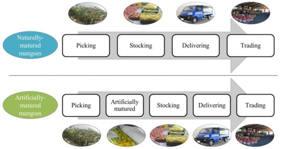
Figure 1.
The harvesting processes of naturally and artificially matured mangoes.
There are different ways to trade mangoes. The first mode is to sell mangoes in a spot market, where buyers negotiate mangoes prices with farmers according to mango qualities and overall supply quantities in the market [5]. The transaction is confirmed whenever the farmer accepts the offer. Since mango demand and supply in Taiwan fluctuate highly, the selling prices usually vary from day to day. The second mode to trade mangoes is the price contract, in which the wholesaler and farmer negotiate a fixed price prior to the harvest season [6]. The contracted price can reduce price variation but is Tless favorable for farmers in Taiwan. This is because the mango qualities differ between different ranches and the contracted price is usually much lower than the selling price in the spot market.
Prior work has considered uncertain factors for making agricultural decisions. For example, scholars analyzed land allocation decisions under uncertain demand [7]. They developed a stochastic programming model with the objective to maximize the probability of satisfying demand. There is a strong correlation between demand and prices for selling mangoes in a spot market. The price of mangoes tends to be lower on days with higher quantities and higher when the trading volume is low. Figure 2 illustrates the selling price and trading quantity on each day for different mango varieties during the harvest season. We found that few papers have developed models to cooperate the inter-effect between demand and supply. This study uses the actual data collected from the Agriculture and Food Agency in Taiwan [8] along with forecasting models to construct the relationship between demand and prices.
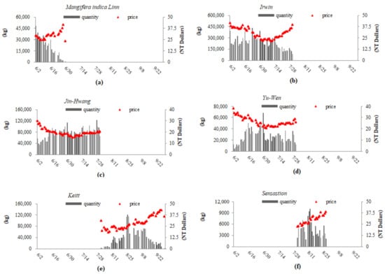
Figure 2.
Trading volumes and selling prices for each mango variety in the spot market. (a), Mangifera indica Linn; (b), Irwin; (c), Jin-Hwang; (d), Yu-Wen; (e), Keitt; (f), Sensation.
During the harvesting season, mango farmers determine how many mangoes to be picked on each day, when to start the artificial maturation operation, and how many mangoes to be sold. These decisions are usually made according to farmers’ experiences. To tackle the increasing uncertainties of price and yield, scholars have suggested risk-sharing strategies, such as insurance [6]. Since this conclusion is based on a questionnaire survey result among farmers in Dutch, these suggested strategies may not be available in our case. In the area of mathematical models, a survey paper highlighted the applications of stochastic programming in supply chain planning under uncertain demands [9]. The authors found that this method can obtain a more realistic cost assessment and can be used to reduce risks in supply chain planning. Other fields’ applications, such as finance, manufacturing, telecommunication, transportation, and energy can be found in another review paper [10]. Among these applications, a common assumption of the stochastic programming model is that the uncertain parameter’s distribution function must be given in order to formulate the deterministic equivalent program and thus the problem becomes computationally trackable. Interested readers may refer to the textbook for a comprehensive review of stochastic programming models and solution approaches for solving each of them [11]. Another approach to model uncertain considerations is robust optimization. Such a model assumes that the variances of uncertain parameters are bounded. Instead of considering the expected performance, the goal is to find the optimal solution considering the worst-case scenario [12]. The drawback of robust optimization is that its decisions may be over-conservative when parameter values are high variance. An application of robust optimization models in agriculture may refer to the wine grape harvest scheduling problem done by Bohle et al. [13].
This study applies the stochastic programming model to explore the operational decisions for mango farmers. Both demand and production yields are predicted via the bass models. The forecast error of each mango variety is assumed to be distributed, where mean and variance are estimated according to the forecast errors. Additionally, we assume that the forecast error distribution is identical and independent on each day during the harvesting season. Uncertain parameters are constructed based on the time-series forecast and forecast error distribution. The stochastic programming model’s objective function minimize the expected cost and constraints capture the precedent operations in a harvesting process as well as resource capacities.
The remainder of this paper organizes as follows. Section 2 provides a review of the related literature in agriculture operational decisions. Section 3 describes the data and models developed for making the mango decision. Section 4 presents the results and optimal strategy. Section 5 provides discussion and conclusions.
2. Literature Review
Harvesting and processing planning have been studied broadly over past decades. An early work analyzed the production schedule for a fresh tomato packing house [14]. Higgins developed models to determine a harvesting schedule to minimize the variability of the daily supply of sugar cane to the mill and variability in daily transportation resource usage [15]. Caixeta-Filho et al. considered the production plan of lily flowers that maximizes net revenue for the farm by taking into account the planting week and expected harvest week [16]. Another work by Caixeta-Filho focused on the orange harvesting scheduling in the juice processing industry [17]. Recently, Vizvári et al. analyzed crop planting decisions with the development of stochastic programs [18]. The crop yield was assumed to be uncertain and cyclic due to the crop’s memory of drought. A chance constraint was formulated to ensure that a certain level of demand is satisfied. Their results suggested that planting crops in a smaller area can provide an extra supply to cover requirements during the low yield season. Another related work studied the crop rotation decision where both yield and demand are fluctuated and uncertain [7]. The objective function is to maximize the probability of demand satisfaction. In the livestock industry, Guan and Philpot analyzed the milk distribution decision in an arborescent supply chain. They developed models to predict milk supplies and used random forecast errors for modeling uncertain parameters in the multi-stage stochastic program [19]. Other researchers assessed the productivity risk under different levels of price settings. A dynamic stochastic programming model was proposed to evaluate both the long-term and short-term rotation strategies for planting crops [20].
Recently, attention has turned to the question about freshness and shelf life effects on agricultural decisions. Ahumada and Villalobos analyzed both harvesting and inventory decisions simultaneously with the consideration of shelf life, where the selling price was assumed to decrease over time for the decaying in the quality of agriculture products [21,22]. The objective maximized the profit under labor force capacity limits. A related work by Ferrer et al. developed a mixed-integer program (MIP) model for grape planting decisions. Their model determined laborer and machine allocations and the sequence of fields to be harvested [23]. The grape quality was formulated as a non-increasing function in time. Similar considerations were studied in another paper by Zhang and Wilhelm [24]. In the area of inventory models, Lodree and Uzochukwu developed a two-period inventory model for fresh products to consider product deterioration, uncertain demand, lead times, and consumer preferences [25]. Additionally, Noparumpa et al. developed models to determine production allocation decisions for a winemaker. They considered both the expected profit and risks of quality rating degradation [26].
We found that prior studies focused on specific operational decisions in the agriculture industry. Yet, none of them have considered the end-to-end process. This study aims to coalesce data analysis and decision models to assess interactions between decisions in different operations. Furthermore, the agriculture product price is strongly correlated with yields. The difference between this study and the related literature is that the relationship between prices and yields is considered in the proposed model, which makes the harvesting decision more realistic. Finally, uncertainties significantly affect agriculture decisions. This study develops stochastic programming model of mango harvesting that explicitly considered uncertain demand, yields, and prices. The next section will explain the detailed procedure of modeling uncertain parameters and the mathematical formulas in stochastic programming.
3. Methods
The harvesting planning comprises a sequence of operational decisions for different varieties of mangoes from June to September. To model uncertain yields and demand, we first apply forecasting to the Bass diffusion model and use time-series trading data in previous years to estimate model parameters. Forecasting errors are calculated using another data set of the testing data. For each mango variety, the forecasting error is assumed to be an independent and identical normal distribution, where its mean value and variance are estimated using forecasting errors obtained beforehand. To model the selling price, a regression model is used to explore the relationship between the price and demand. The contents of this section firstly describe key features and parameters for each mango variety. Then, we explain the data collection approach and how the uncertain parameters are set up using fitting results. The last subsection presents the stochastic programming model.
3.1. Data and Assumptions
This study considers the common varieties of mangoes in Taiwan, and each of them has a different maturation process, picking schedule, and inventory time limit. The naturally matured mangoes (including Mangifera indica Linn and Irwin) have a short shelf life at room temperature, and the farmer must sell the mangoes within two days. Artificially matured mangoes (including Jin-Hwang, Yu-Wen, Sensation, and Keitt) can be stored for a long time at ambient temperature before being artificially ripened. The harvest timing varies from year to year. Figure 3 displays the sales data collected from Tainan County between June and September 2015. The line chart shows the weekly sales volume for each mango variety, and the pie chart depicts the proportion of sales volume. The harvest season starts in June and ends by the end of September. The highest volume occurs in the fourth week of June. Additionally, most trading takes place in June and July, and August and September contain less than one-fifth of the entire volume. Irwin has the most trading volume among the six mango varieties, which accounts for more than 60% of the overall volume. In comparison, Jin-Hwang is the second-highest product with a 20% market share.
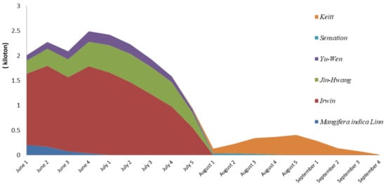
Figure 3.
The weekly trading volume and market share of each mango variety during a harvesting season.
Table 1 summarizes the major characteristics of mangoes considered in this study. Mangifera indica Linn and Irwin are naturally matured mangoes. The other mango varieties must perform artificial maturation, which will take 48 to 72 h to have about 90% of mangoes matured under ambient temperature, and the duration depends on mango varieties and sizes [2]. In the case study, we assume all artificially matured mangoes will be matured for three days. The season for picking Mangifera indica Linn starts from the beginning of June until the end of July, and for Irwin, Jin-Hwang, and Yu-Wen it starts between June and August. The Sensation and Keitt picking seasons are between August and September.

Table 1.
Maturing varieties and picking time windows for different mango varieties.
3.2. Time-Series Forecasts and Forecast Error Analysis
This section describes how the distributions of uncertain parameters for the stochastic programming model are constructed. Mango demand will grow rapidly with the increase in productivity at the beginning of the season. Once the peak is passed, the demand will begin to shrink exponentially. Such a pattern can well fit by the use of the Bass diffusion model [27]. We segregate trading data by mango varieties and use each of them to estimate model parameters separately.
Let f (t) be the density of adopters at time period t with an associated cumulative distribution F (t). Notation p represents the coefficient of innovation (or external influence) and q is the coefficient of imitation (or internal influence). Thus, the proportion of demand not being at time period t is equal to the portion of new innovator and new imitator as the following equation We further denote m as the total demand of adopters, as the number of adopters at time t defined as , and the cumulative demand of adopters at period t as . Hence, the number of new adopters can be determined by . Let be the cumulative adopters and be the new ones observed at time t. The estimation of new adopters is as the following equation: The objective of the estimation is to find the parameter values of p and q such that the total error is minimal. The actual trading volume is aggregated on a weekly basis for fitting the forecasting models.
Table 2 shows the estimated parameters in the Bass model for each mango variety. As a result, all ratios are greater than one (the smallest value is 2.0 for Mangifera indica Linn and the largest ratio is 28.1 for Keitt). It implies that the demand increases or decreases exponentially over time. Additionally, the sales volume in the previous time period has positive effects (i.e., ).
Table 2.
The fitting results of internal influence and external influence factors.
The Bass models perform well in capturing demand trends during the harvesting season. Figure 4 shows the actual and forecast trading volumes for different mango varieties. As one can tell, the model can precisely predict the start time, peak time, and end time of each mango variety. Except for Jin-Hwang, Sensation, and Keitt mangoes, the predicted peak volume is very close to the actual situation. We further analyze the accuracy of the Bass model. Table 3 shows the Mean Absolute Percentage Error (MAPE) and Mean Square Error (MSE) of each mango variety, where MAPE is defined as the ratio of the expectation of absolute errors divided by actual demand and MSE is defined as . The MAPEs of Mangifera indica Linn, Jin-Hwang, and Yu-Wen are less than 20%, Irwin and Keitt are about 30%, and Sensation performed the worst at 40%. The ranking of the MSE of the six mango varieties is opposite to that of MAPE, in which Sensation has the smallest value, and Irwin has the largest value. Because Sensation has the least actual demand, the denominator of MAPE is small, resulting in the worst MAPE. In fact, the forecasts for all mango varieties performed well and are close to actual demand.
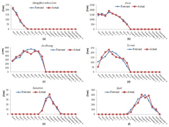
Figure 4.
Comparing the trading volumes of actual and forecast in a time series. (a), Mangifera indica Linn; (b), Irwin; (c), Jin-Hwang; (d), Yu-Wen; (e), Sensation; (f), Keitt.
Table 3.
The Bass model MAPE performances.
3.3. Stochastic Programming Model
Stochastic programming has been widely applied for analyzing the optimal decision under uncertain environments [10]. In this study, demand, yield, and price are considered as random variables, the probability distribution of which has been explained in the foregoing subsection. The objective is to minimize the expected cost, which includes inventory cost, shipping cost, artificial maturing cost, and sales revenue across all mango varieties during the multi-month harvest season. The decision variables involve picking quantity, inventorying quantity, artificial maturation quantity, shipping quantity, and sales volume on each time period. Table 4 summarizes notations used in the stochastic programming model.
Table 4.
Notations.
Figure 5 illustrates our ideas to formulate the MIP model, where the flow chart at the top represents the harvesting process for naturally matured mangoes, and another one is for artificially matured mangoes. Each rectangular block represents either picking, artificially maturing, shipping, or trading operation in both flow charts, while trapezoid blocks represent stocking mangoes with various statuses. The directed edge represents the sequence to perform two consecutive operations. Most blocks are connected by less than or equal to one incoming and outgoing arc, except for the operations of picking and stocking matured-and-unsold artificially matured mangoes. Since the farmer can defer artificial maturing decisions, two outgoing arcs depart from the picking operation. Another block with multiple outgoing arcs is the matured-and-unsold stocking, in which the solid outgoing arc represents the first attempt of farmers to deliver and sell the one-day-old mangoes, and the dashed outgoing arc is the second attempt for dealing with the two-day-old mangoes. Additionally, two incoming arcs connect to the matured and unsold stocks, where the sold arc represents the influx of one-day-old mango, and the dashed arc is the returning unsold mangoes.
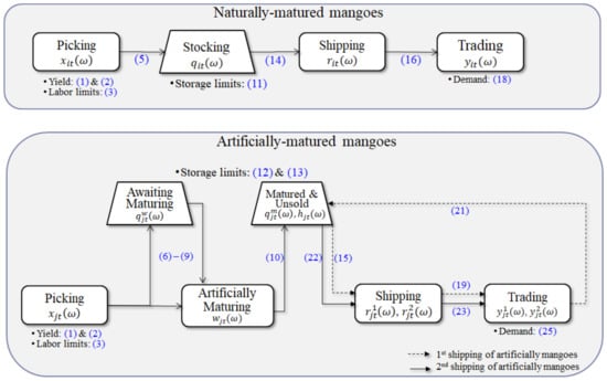
Figure 5.
Illustrating the relationship between constraints and decision variables in the proposed stochastic programming model.
The stochastic programming model of mango harvest and distribution is as follows:
Subject to
| (1) | ||
| (2) | ||
| (3) | ||
| (4) | ||
| (5) | ||
| , | (6) | |
| (7) | ||
| (8) | ||
| (9) | ||
| (10) | ||
| (11) | ||
| (12) | ||
| (13) | ||
| (14) | ||
| (15) | ||
| (16) | ||
| (17) | ||
| (18) | ||
| (19) | ||
| (20) | ||
| (21) | ||
| (22) | ||
| (23) | ||
| (24) | ||
| (25) | ||
| (26) | ||
| All decision variables are nonnegative. | (27) | |
The objective function is to minimize the expected costs, where the first and second terms represent the inventory cost and transportation cost of artificially matured mangoes, respectively. The third term accounts for the inventory cost of one-day-old artificially matured mangoes. The fourth term represents the inventory cost of two-day-old artificially matured mangoes. Since the freshness will decay over time, we set a higher inventory cost of artificially matured mangoes than mangoes waiting artificially matured (i.e., ). The fourth term accounts for the shipping cost of one-day-old artificially matured mangoes. The fifth term is the inventory cost of unsold mangoes. These mangoes must return to the farmer and then ship to the market on another day. Additionally, a third trip may need for returning the unsold two-day-old mangoes, and therefore, the total shipping cost of two-day-old artificially matured mangoes is modeled as three times of per-unit shipping cost . The terms and account for the total sales incomes of selling naturally matured mangoes and artificially matured mangoes, respectively.
In Constraints (1) and (2), the picking quantity must be less than or equal to the number of mangoes ready to be harvested. Since the picking decision can delay for one day, the right hand side of constraints (2) includes both yield and unpicked mangoes in the previous time period. Constraint (3) considers the capacity limit of picking mangoes at each time period. Constraint (4) is used to compute the number of unpicked mangoes , which is equal to yield minus picking quantity. Constraint (5) ensures that the inventory quantity of naturally matured mangoes is equal to the picking quantity .
The artificially matured mango can be preserved for a long time before maturity. Constraints (6) and (7) determine the inventory quantity of mangoes waiting for artificial maturation , equal to the previous inventory plus picking quantity , and then minus artificially matured quantity . Constraints (8) and (9) ensure that the ripening quantity cannot exceed inventory and picking. Constraints (10) and (11) compute inventory of mangoes that have artificially matured. Since the maturing process takes three days, the inventory levels in the first three time periods are zeros (. In Constraint (11), the is equal to the artificially matured quantity three days ago, plus previous inventory, and then minus the shipping quantity of one-day-old matured mangoes .
The artificially and naturally matured mangoes are kept separately. Constraint (12) ensures that the total inventory of naturally matured mangoes is less than or equal to the warehouse capacity . In Constraint (13), the inventory level of artificially matured mangoes in the first three days, equal to mangoes waiting to be matured plus the total amount of ripening from the first day to the present, cannot exceed the maximal capacity . Similarly, the left-hand side in Constraint (14) determines the inventory levels on the fourth day and after cannot exceed the capacity limit, where the mango inventory is equal to the mangoes waiting to be mature, the mangoes in ripening, the mangoes that have matured, and minus unsold one-day-old mangoes. Figure 6 is a numerical example to explain the left-hand-side formulations in Constraints (13) and (14). Suppose that seven mangoes are picked on the first day, and two of them are ripening. Therefore, there are five unripened mangoes and the total inventory at the end of the day is seven. Five mangoes are harvested on the second day, and thus the total inventory is twelve, including the first day’s harvest. Additionally, assuming that two mangoes are beginning to ripen, and therefore the total ripening mangoes are four, two of which are one day old matured and two are two days old matured. On day five, the inventory level includes mangoes picked from day one to day four, and then subtracts two mangoes ripened on day one and sold on day five.
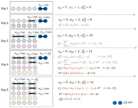
Figure 6.
The numerical example to illustrate the inventory levels of artificially matured mangoes defined at the left-hand-sides in Constraints (13) and (14).
Constraint (15) ensures that the shipping quantity of naturally matured mangoes is less than or equal to the inventory in the previous time period to account for lead-time of inventory and transportation operations. Constraint (16) ensures that the quantity to deliver one-day-old artificially matured mangoes cannot exceed the ripened mangoes. Constraint (17) ensures that the naturally matured mango selling quantity is less than or equal to the shipping quantity. Constraints (18) ensures the naturally matured mangoes selling quantities are less than or equal to the demand. Constraints (19) ensure that the selling quantity of one-day-old artificially matured mangoes is less than or equal to the shipping quantity. Constraints (20) and (21) determine the number of unsold one-day-old mangoes, which is zero in the first three days, and then defined as shipments minus sales. In Constraints (22) and (23), the number of two-day-old mangoes is zero in the first four days or no more than stocks after the fourth day. Similarly, Constraints (24) and (25) specify the boundary of selling two-day-old mangoes each day. In Constraint (26), the total sales of one-day-old and two-day-old mangoes cannot exceed the demand.
4. Results
We use the forecasts and forecast error distributions to construct the probability distribution of the uncertain parameters of the stochastic programming model. The forecast error at each time period follows an independent and identical normal distribution, where the mean and standard deviation are estimated from the testing data set. The demand and yield at each time period are generated using forecasts and forecast error distributions, both of which are sampled from the same probability distribution but sampled separately. In addition, the mango price is generated by a linear function of mango demand, where its parameters are fitted by the same data set used to build the forecast model. It is worth mentioning that the fitting results show an opposite relationship between the sales price and trading volume of all mango varieties, and this trend is the same as that of most fresh products.
4.1. Convergence Analysis of SAA
The sampling sizes of uncertain parameters affect both the model accuracy and the runtime to solve stochastic programs. Models using larger sample sizes provide a better approximation, but they are usually more difficult to solve. There is no clear way to determine the best sampling size. We implement the sample average approximation (SAA) to obtain a good quality solution in time for the proposed stochastic programming model [10]. The algorithm samples coefficients in both objective function and constraints and then resolves the new sampled problems iteratively. The optimal objective value will stabilize once the sample size increased to a sufficient number. We stop the algorithm when the gap of objective values in two consecutive iterations is less than a tolerated value. Figure 7 displays the expected profit (that is, the objective value multiplied by −1) of stochastic programs in different sample sizes. The objective value decreases as the sample size increases, and when the same size increases to forty, it will stabilize at about five million.
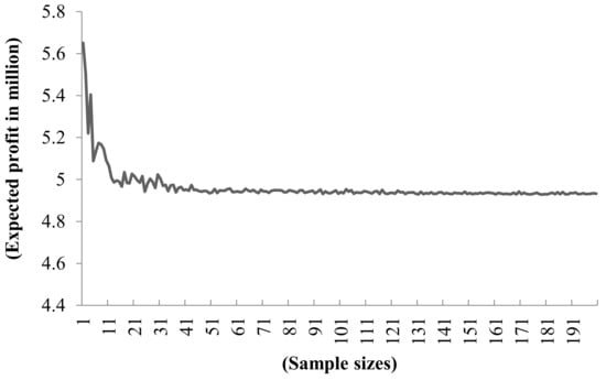
Figure 7.
The expected profits of stochastic program solutions with different sample sizes.
In the following analysis, we use a sample size of two hundred. We believe that such a sample size would provide relatively robust results, and similar findings would be concluded even using larger sample sizes.
4.2. Comparing Deterministic and Stochastic Solutions
This section compares the deterministic and stochastic models to assess the value of stochastic solutions and understand the impact of uncertain forecast errors on profits. The benchmark model, known as the expected value (EV) model, is formulated as a deterministic mathematical program using the expected values of uncertain parameters. The EV solution is then applied to each sampled problem instance to obtain the expectation of expected value solution (EEV). For minimization problems, the stochastic program solution is less than or equal to EEV. This is because the EV solution is suboptimal (or even infeasible) for each sampled problem instance. The value of stochastic solution (VSS), defined as EEV–SP, represents the potential loss of profit for mango farmers using the expected value to make harvest decisions. Another implication is the impact of uncertain forecast errors on profits. Our analysis uses two hundred randomly generated scenarios, and the results are shown in Table 5. The objective function is to minimize the total cost. Thus, a smaller objective value means a more profitable solution. The EV objective value (approximately minus 5.8 million) is less than SP, but when the EV solution applies to all other scenarios, the expected objective value is −4,911,662. Therefore, EV is about 20% higher than EEV (from −5,816,137 to −4,911,662). This implies that the EV objective value is too optimistic and may mislead decision-makers. In contrast, if decision-makers adopt the SP solution rather than EV, they can increase profit by USD 50,252.
Table 5.
Comparing expected-value model and stochastic program model solutions.
4.3. The Optimal Harvest Planning
The SP solution provides abundant information about the timing and quantities of each operational decision. Table 6 is the color code of each operation that will be used for presenting the optimal harvest planning in Table 7. Due to the limitation of manuscript length, Table 7 only contains the optimal quantity for picking, stocking, delivery, and sales in June. In these tables, each cell shows the lower and upper limits of the best solution in all scenarios. For example, the picking quantities of Mangifera indica Linn on 5 June are between 11 and 13 tons. If there is only a single value in a cell, it means that all scenarios obtain the same solution.
Table 6.
Color coding for different operations.
Table 7.
The optimal harvest decision for the stochastic program in June. Different color codes indicate different operations, as defined in Table 6. The numbers in each cell refer to the minimal and maximal solutions in all scenarios (unit: ton).
In Table 7, the Mangifera indica Linn is the earliest harvested mango, and its season starts at the beginning of June. All mangoes are delivered and sold on the next day after they are harvest. Another naturally matured mango, Irwin, is harvested from the end of June. Similar to Mangifera indica Linn, they are sold one day after harvest. For artificially matured mangoes, Yu-Wen mangoes are picked in early June, and Jin Hwang mangoes are harvested from 18–21 June Both mango varieties are ripened on the harvest day. Additionally, all mangoes are sold when the ripening process is complete.
5. Discussion and Conclusions
This study integrated forecasting and mathematical programming models for making mango harvest decisions in Taiwan. We addressed important concerns in the agriculture industry where demand and supply are highly uncertain. A time-series model was developed to forecast the demand and supply of different mango varieties using actual trading data in Taiwan. Additionally, a stochastic programming model was developed to determine the optimal picking, ripening, stocking, shipping, and selling decisions. The SAA was implemented for solving the stochastic program, and the computational result showed that the algorithm could obtain a quality solution in time. We conducted a case study to assess the value of stochastic solutions, where the stochastic programming model obtained more profitable solutions than the deterministic model used expected values. Finally, we organized the overall harvest plan according to the optimal solution to help farmers prepare resources in advance. Using our approaches would benefit growers to better arrange labor resources by balancing workloads during the harvesting season and better utilize resources for stocking picked mangos. Additionally, the model can be used for what-if analysis over different marketing situations to maximize the grower’s revenue. As a result, the farm operations will be more efficient and reduce the risk due to climate or demand changes.
Our findings and suggestions are as follows. The workforce requirement to pick mangoes in June is higher than July and August. This is because the harvest time of naturally matured mangoes is in June, and the harvest time cannot be changed. Thus, it is recommended to plant more mango varieties to alleviate peak labor requirements. The naturally matured mangoes require less storage space because they are sold immediately after harvest. In contrast, more storage space should be planned for stocking artificially matured mangoes to increase operational flexibility.
The limitation of this study is that we only consider operational decisions during a harvest season. Agriculture decisions in the early stage can have impacts. For example, mango yield quantity and timing are related to fruit bagging and pollination decisions made before the harvest season. A potential extension of our work is to include the above considerations to provide fruit farmers with more comprehensive planning. Additionally, we have considered the operational decisions of individual farmers, but incorporating competition among different decision-makers into the model is still an open issue. In our model, the price is an uncertain parameter whose trend is opposite to the total trading volume in the market. This approach may only capture competition among farmers to a certain extent. Considering the interaction between decision-makers will be an important direction for future research. Finally, using model-based approaches can more accurately capture the relationship between input and out variables to analyze a complex system, and their applications improve the efficiency of agricultural operations [28]. Our attempt to apply model-based methods for predicting yields coupled with mathematical programming models offers advantages to allow agriculture preparation. However, the choice of model-based models may depend on the type and extent of data that are available for use in forecasting.
Author Contributions
Conceptualization, S.-I.C. and W.-F.C.; methodology, S.-I.C. and W.-F.C.; software, S.-I.C. and W.-F.C.; validation, S.-I.C.; formal analysis, S.-I.C. and W.-F.C.; investigation, S.-I.C. and W.-F.C.; resources, S.-I.C.; data curation, S.-I.C. and W.-F.C.; writing—original draft preparation, S.-I.C. and W.-F.C.; writing—review and editing, S.-I.C.; visualization, S.-I.C. and W.-F.C.; supervision, S.-I.C.; project administration, S.-I.C.; funding acquisition, S.-I.C. Both authors have read and agreed to the published version of the manuscript.
Funding
This research was funded by Ministry of Science and Technology, Taiwan (https://www.most.gov.tw/), grant 109-2221-E-009-065.
Institutional Review Board Statement
Not applicable.
Informed Consent Statement
Not applicable.
Data Availability Statement
Not applicable.
Acknowledgments
The authors would like to thank Yu-Chen Cheng for reformatting the final version of the manuscript.
Conflicts of Interest
The authors declare no conflict of interest.
References
- Analysis of the Competitiveness of Domestic Mango Industry. 2002. Available online: https://www.coa.gov.tw/ws.php?id=4299 (accessed on 18 August 2021).
- Mango Management Technical Report. 2013. Available online: https://book.tndais.gov.tw/Brochure/tech156.pdf (accessed on 18 August 2021).
- Cantwell, M.; Suslow, T. Lettuce, Crisphead: Recommendations for Maintaining Postharvest Quality. 2002. Available online: http://postharvest.ucdavis.edu/Commodity_Resources/Fact_Sheets/Datastores/Fruit_English/?uid=37&ds=798 (accessed on 18 August 2021).
- Agricultural Knowledge Portal. Mango Processing after Harvest. Agriculture and Food Agency, Council of Agriculture, Executive Yuan, Taiwan. Available online: https://kmweb.coa.gov.tw/subject/index.php?id=19 (accessed on 19 April 2017).
- Mendelson, H.; Tunca, T. Strategic spot trading in supply chains. Manag. Sci. 2007, 53, 742–759. [Google Scholar] [CrossRef]
- Meuwissen, M.; Hardaker, J.; Huirne, R.; Dijkhuizen, A. Sharing risks in agriculture; principles and empirical results. NJAS-Wagening. J. Life Sci. 2001, 49, 343–356. [Google Scholar] [CrossRef]
- Vizvári, B.; Lakner, Z. A stochastic programming based analysis of the field use in a farm. Ann. Oper. Res. 2014, 219, 231–242. [Google Scholar] [CrossRef][Green Version]
- The wholesale trading market of agricultural products. Agriculture and Food Agency, Council of Agriculture, Executive Yuan, Taiwan. Available online: http://amis.afa.gov.tw/ (accessed on 19 April 2017).
- Gupta, A.; Maranas, C.D. Managing demand uncertainty in supply chain planning. Comput. Chem. Eng. 2003, 27, 1219–1227. [Google Scholar] [CrossRef]
- Birge, J.R. Stochastic programming: Computation and applications. INFORMS J. Comput. 1997, 9, 111–133. [Google Scholar] [CrossRef]
- Birge, J.R.; Louveaux, F. Introduction to Stochastic Programming, 2nd ed.; Springer Science & Business Media: New York, NY, USA, 2011. [Google Scholar]
- Ben-Tal, A.; El Ghaoui, L.; Nemirovski, A. Robust Optimization; Princeton University Press: Princeton, NJ, USA, 2009. [Google Scholar]
- Bohle, C.; Maturana, S.; Vera, J. A robust optimization approach to wine grape harvesting scheduling. Eur. J. Oper. Res. 2010, 200, 245–252. [Google Scholar] [CrossRef]
- Miller, W.A.; Leung, L.C.; Azhar, T.M.; Sargent, S. Fuzzy production planning model for fresh tomato packing. Int. J. Prod. Econ. 1997, 53, 227–238. [Google Scholar] [CrossRef]
- Higgins, A.J. Australian sugar mills optimize harvester rosters to improve production. Interfaces 2002, 32, 15–25. [Google Scholar] [CrossRef]
- Caixeta-Filho, J.V.; van Swaay-Neto, J.M.; Wagemaker, A.D.P. Optimization of the production planning and trade of lily flowers at Jan de Wit Company. Interfaces 2002, 32, 35–46. [Google Scholar] [CrossRef]
- Caixeta-Filho, J.V. Orange harvesting scheduling management: A case study. J. Oper. Res. Soc. 2006, 57, 637–642. [Google Scholar] [CrossRef]
- Vizvári, B.; Lakner, Z.; Csizmadia, Z.; Kovács, G. A stochastic programming and simulation based analysis of the structure of production on the arable land. Ann. Oper. Res. 2011, 190, 325–337. [Google Scholar] [CrossRef]
- Guan, Z.; Philpott, A.B. A multistage stochastic programming model for the New Zealand dairy industry. Int. J. Prod. Econ. 2011, 134, 289–299. [Google Scholar] [CrossRef]
- Ridier, A.; Chaib, K.; Roussy, C. A dynamic stochastic programming model of crop rotation choice to test the adoption of long rotation under price and production risks. Eur. J. Oper. Res. 2016, 252, 270–279. [Google Scholar] [CrossRef]
- Ahumada, O.; Villalobos, J.R. Operational model for planning the harvest and distribution of perishable agricultural products. Int. J. Prod. Econ. 2011, 133, 677–687. [Google Scholar] [CrossRef]
- Ahumada, O.; Villalobos, J.R.; Mason, A.N. Tactical planning of the production and distribution of fresh agricultural products under uncertainty. Agric. Syst. 2012, 112, 17–26. [Google Scholar] [CrossRef]
- Ferrer, J.C.; Cawley, A.M.; Maturana, S.; Toloza, S.; Vera, J. An optimization approach for scheduling wine grape harvest operations. Int. J. Prod. Econ. 2008, 112, 985–999. [Google Scholar] [CrossRef]
- Zhang, W.; Wilhelm, W.E. OR/MS decision support models for the specialty crops industry: A literature review. Ann. Oper. Res. 2011, 190, 131–148. [Google Scholar] [CrossRef]
- Lodree, E.J., Jr.; Uzochukwu, B.M. Production planning for a deteriorating item with stochastic demand and consumer choice. Int. J. Prod. Econ. 2008, 116, 219–232. [Google Scholar] [CrossRef]
- Noparumpa, T.; Kazaz, B.; Webster, S. Wine futures and advance selling under quality uncertainty. Manuf. Serv. Oper. Manag. 2015, 17, 411–426. [Google Scholar] [CrossRef]
- Bass, F.M. A new product growth for model consumer durables. Manag. Sci. 1969, 15, 215–227. [Google Scholar] [CrossRef]
- Cook, S.E.; Bramley, R.G.V. Precision agriculture: Opportunities, benefits and pitfalls of site specific crop management in Australia. Aust. J. Exp. Agric. 1998, 38, 753–763. [Google Scholar] [CrossRef]
Publisher’s Note: MDPI stays neutral with regard to jurisdictional claims in published maps and institutional affiliations. |
© 2021 by the authors. Licensee MDPI, Basel, Switzerland. This article is an open access article distributed under the terms and conditions of the Creative Commons Attribution (CC BY) license (https://creativecommons.org/licenses/by/4.0/).