1. Introduction
Air pollution is one of the major issues plaguing the world today, which highly correlates with vast industrialization, in addition to the already existing particulate matter pollutants [
1,
2,
3]. There are a variety of air pollution compositions, but the majority contain PM2.5 and PM10 particulate matter. PM2.5 in particular (with a diameter of 2.5 μm), has been shown to be harmful to humans based on several epidemiological studies [
3,
4,
5,
6]. Due to this, experts put an emphasis on PM2.5 when performing air quality monitoring.
In general, particulate concentration measurements are done by dedicated monitoring stations that are geographically dispersed [
7,
8,
9]. Jumaah et al. [
10] found such dispersions to be problematic as insufficient samples might be collected to come up with any meaningful analysis. This is supported by Zhao et al. [
11] and Hsu et al. [
12], where both assert the importance of more comprehensive area coverage to allow reliable and continuous sampling.
In addition to location, gauging pollution levels in the chronological structure of a particular pollutant, such as PM2.5, is highly influenced by atmospheric factors and noise. Studying the influence or correlation of such variables on particulate matter can provide insights for better pollution monitoring [
13]. The work in [
14], for instance, asserts that the correlation between particulate matter and traffic noise should be looked into for better air pollution insights. This is supported by [
15], where their work demonstrated how various air contaminants along with noise led to worsened air quality. In addition to traffic (as the main cause of noise pollution), weather can be an influential periodic factor that produces seasonal variations of noise [
16].
1.1. Noise Pollution Mapping
Chandrappa and Das [
17] define noise as undesired sound. As of 2016, the World Health Organization (WHO) puts noise contamination as the third greatest environmental contamination after air and water [
18]. Studies have shown the adverse impacts of noise on human health, such as being destructive to human hearing [
19]. Therefore, it is sensible to reduce (or even eliminate) unnecessary noise for the overall well-being of humanity [
20,
21].
Advancements in noise pollution mapping has facilitated in noise pollution assessment. Since such maps display the spatial distributions of noise, one can map noise at different times of the day such as in the morning, mid-day, evening, and night [
22]. This allows researchers and authorities to evaluate locations containing possible noise pollutions and decide on necessary actions. One practical application is the analysis and assessment of traffic noise contamination [
23]. In other research, noise mapping is performed through interpolating data from different monitoring stations where noise pollution can then be assessed through equivalent sound pressure data [
24]. An example of such work was done by Harman et al. [
25] where the noise map of Isparta city was generated using inverse distance weighted (IDW), Kriging, and multiquadric interpolation methods using various parameters. Location-wise noise analysis was then assessed based on national environmental noise thresholds. The most applied methodology has always been getting information on the features of various sample points as much as possible in the particular geographic region, as well as predicting the value of the unobserved point from the value of the known point over spatial interpolation [
26].
1.2. Geographical Information Systems (GIS)
Environmental modeling possesses significant history and progress, and has many applications in problems related to ecology [
27]. Urban ecological problems relate to studying wide areas that take advantage of geographical information systems (GISs) [
28]. GISs are able to incorporate various information sources allowing data interpretation through various modeling and visualization techniques [
29]. Hence, GISs can be considered decision support systems for the relevant authorities to perform assessments and decision making [
30,
31,
32,
33]. The use of spatial modeling and statistics has risen up-to-date [
34]. Multiple new techniques for the statistical assessment and model patterns have been developed currently [
35]. For example, modeling air quality is helpful in air pollution problems controlling [
36].
In this study, we evaluate air quality and determine noise distributions in silent zones inside Tikrit University, Tikrit, Iraq. Building upon GIS techniques, we apply the least-square model to investigate the impact of noise and meteorological factors on air pollution and PM2.5 prediction. Specifically, the correlation between noise with climatic parameters (i.e., as independent variables) is examined in a multivariate regression model for the PM2.5 particulate quantity estimation. Our data consist of daily manually measured data around Tikrit University (during July 2019) as well as NASA satellite remotely sensed data of PM2.5. The month of July is characterized by high temperatures throughout Iraq, and the university is devoid of students. Therefore, it is possible to determine the extent of noise pollution with the least amount of sound and the extent of the impact of atmospheric factors at peak times. Moreover, we can determine the extent of noise from the university’s surroundings. We expect this study to offer insights for the proposal of future air quality management protocols in the study area and the city of Tikrit.
2. Materials and Methods
2.1. Study Area
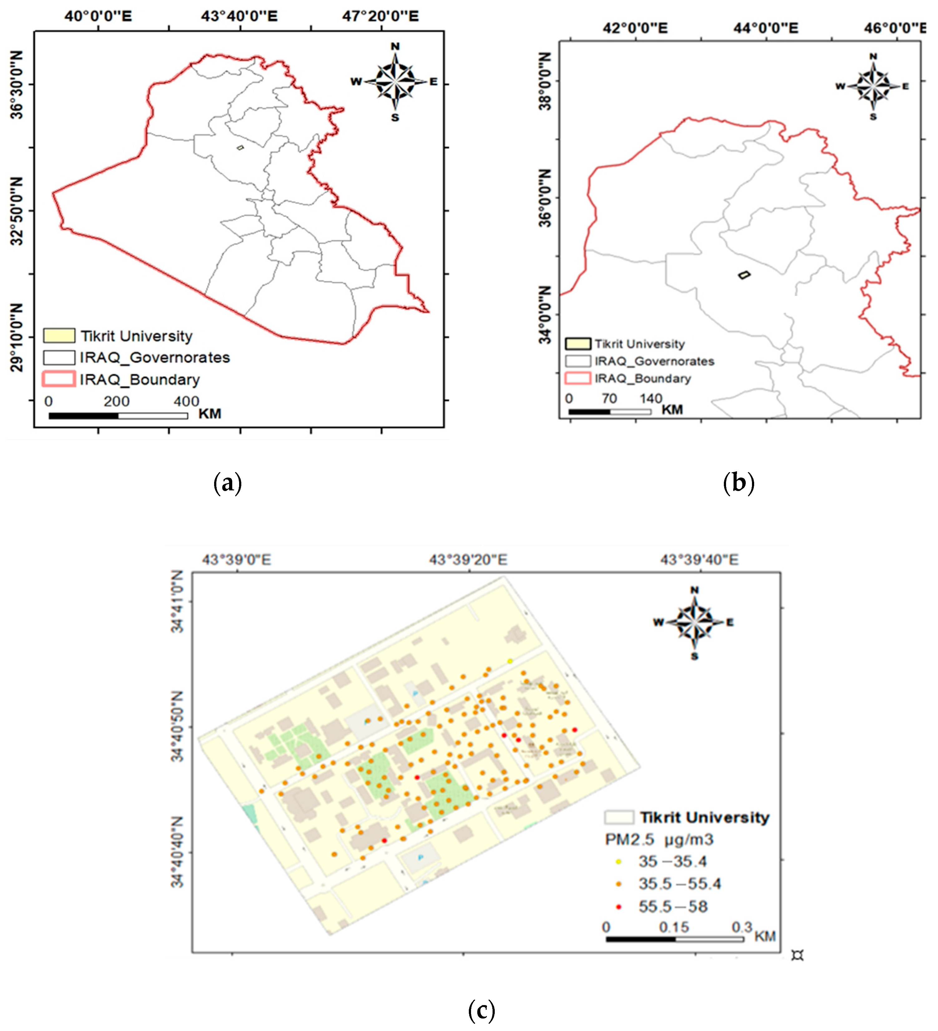
Tikrit University is chosen as the study area. It is located in Tikrit city, situated in the Salahuddin province of Iraq, which is 155 km from the capital city of Baghdad [
37]. The study area (
Figure 1) lies between 43°38′56.4″–43°39′35.5″ E and 34°40′33.3″–34°41′2.4″ N. The main goal of this study is to evaluate the environmental impacts of air and noise pollution occurring inside the university area. Tikrit University is selected due to the fact that it is an important educational region.
2.2. Data Acquisition and GIS Techniques
Measurements were taken along the study area, which consist of the following:
The overall amassed dataset was then processed using ArcGIS10.3. Two methods were used to represent the data distribution, namely the IDW and least square modeling (LSM).
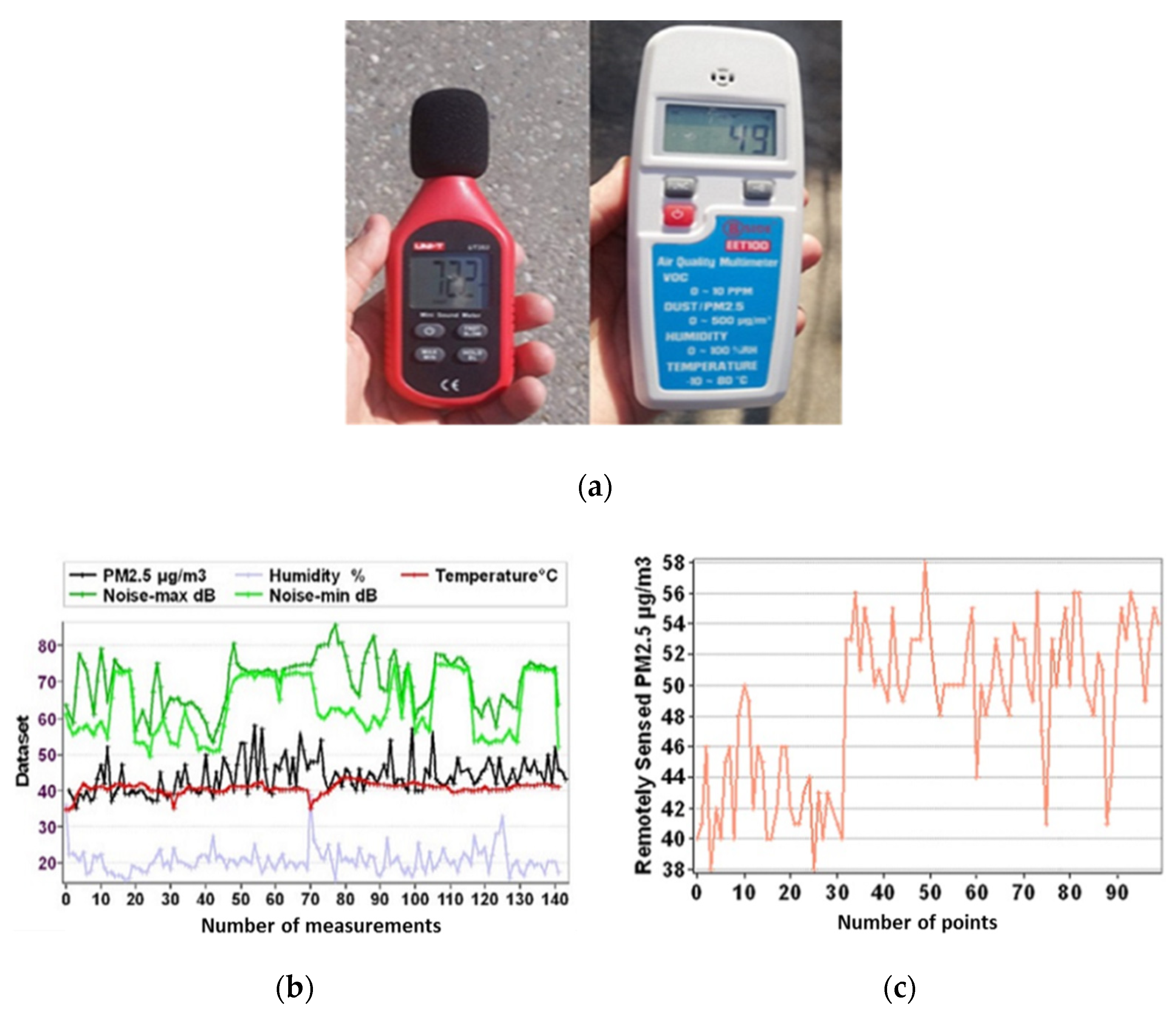
Figure 2 shows the details of data acquisition/data types, along with the measuring devices that were used (i.e., mini sound meter and air quality multimeter).
In this study, noise levels were measured using the mini sound meter. Fieldwork involved measuring the maximum noise and minimum noise pollutions inside the university and surrounding areas, which were conducted throughout July 2019. For each sampling site, noise measurements were continuously taken for 30 days. The data collected from each location were processed for statistical analysis.
The data that belong to noise pollution are shown in
Figure 2b, which depict the average values of maximum and minimum noise levels in the silence zone of Tikrit city at various time intervals (i.e., 9:00 a.m., 11:00 a.m., 2:30 p.m., and 4:30 p.m.). Weather data (temperature and humidity) were measured by the air quality multimeter. To validate our results, historical data of PM2.5 levels were obtained from air matter, which was provided by the Global Air Quality Service Provider and downloaded from
https://air-matters.com/ (accessed on 20 September 2019).
To assess and evaluate the influence of noise and air pollution, the IDW interpolation technique was employed. This method was chosen due to its suitability in flat lands where there is uniformity between the variables. As IDW is a statistical technique, each known point is assumed to affect the magnitude of unknown points. Therefore, the values of points near the known points can be calculated [
4,
38]. Note that the unknown points’ values can be deduced, but with the risk of low accuracy. This is due to the fact that values of converging points searched by IDW can vary significantly. Therefore, interpolated point values were collected in small and closely adjacent areas, ensuring higher point distribution accuracy. The equation for IDW and estimation of
at (
) can be written as Equation (1):
where
denotes the control value for the
th sample point, and
is a weight that defines the relative importance of the specific control point
in the interpolation process [
30]. The IDW analysis is generated based on the concept of spatial dependence making it a reliable interpolation process for air pollution status prediction. IDW also measures the ratio of the dependency relationships between adjacent and discrete features and specifies the result of the cell in the segment that requires metadata.
After performing IDW, two empirical linear models are applied to the results where the first model is constructed based on 100 points from the field data, whereas the second model is constructed based on remotely sensed PM2.5 data. As for the image properties, moderate resolution imaging spectroradiometer (MODIS) images were downloaded at a 30 m resolution per pixel, since 7 July 2019 with WGS 84 projections.
2.3. Linear Regression
Linear regression is a statistical prediction technique that models the linear dependence/relationship between a variable with other variables (known as explanatory variables). Based on training/observed data, a linear fit (i.e., the linear model) is estimated through an iterative process of parameter/coefficient updates. These parameters are updated based on the concept of error reduction between each iteration’s predicted value (i.e., hypotheses) and the respective known value in the dataset. Once the overall error is minimized, the linear model is considered converged and ready to be deployed. The model we generated correlates PM2.5 to the noise and weather data (i.e., the two explanatory variables) to predict PM2.5 values in the specified region inside the university. This means that the model takes in as input, real-world (previously unseen by the model during training) values of the explanatory variables to estimate the PM2.5 response. If the purpose is to interpret the changes in the response features that can be related to changes in the explanatory features, linear regressions can be used to determine the power of the correlation within the dependent and the explanatory features. Moreover, particularly to ascertain if some of the explanatory features may not have a linear relation with the response ever or to distinguish if any subset of explanatory features may include irrelevant information of the response [
39].
Since we consider two explanatory variables (factors), the multiple linear regression (least-squares) is used. Additionally, we used Cook and Weisberg [
4], Weisberg [
40], Sen and Srivastava [
41], and Jumaah et al. [
42]. The multiple least-squares regression can be represented by Equation (2).
where
represents a point location,
is the estimated factor at
,
are the explanatory factors at
,
is the intercept term,
are the factor coefficients, and
is the error term.
3. Results
3.1. Resultant Distribution Maps
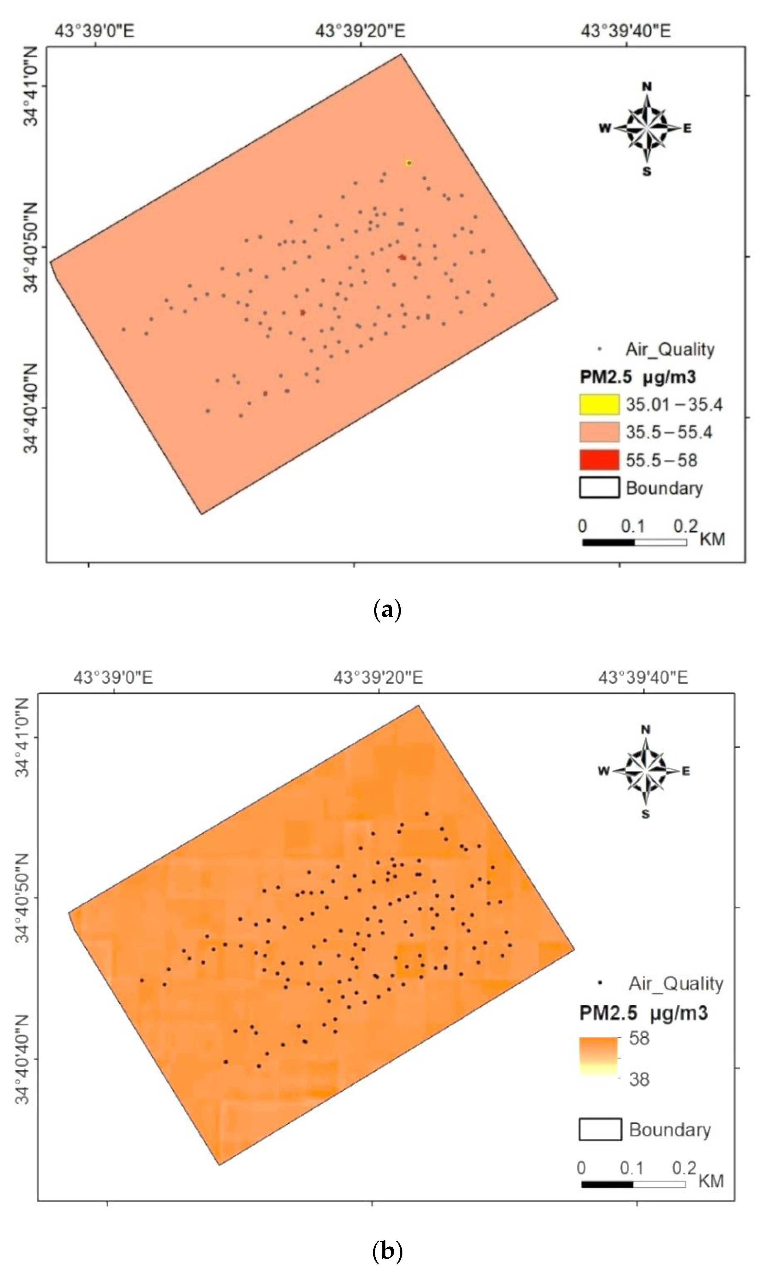
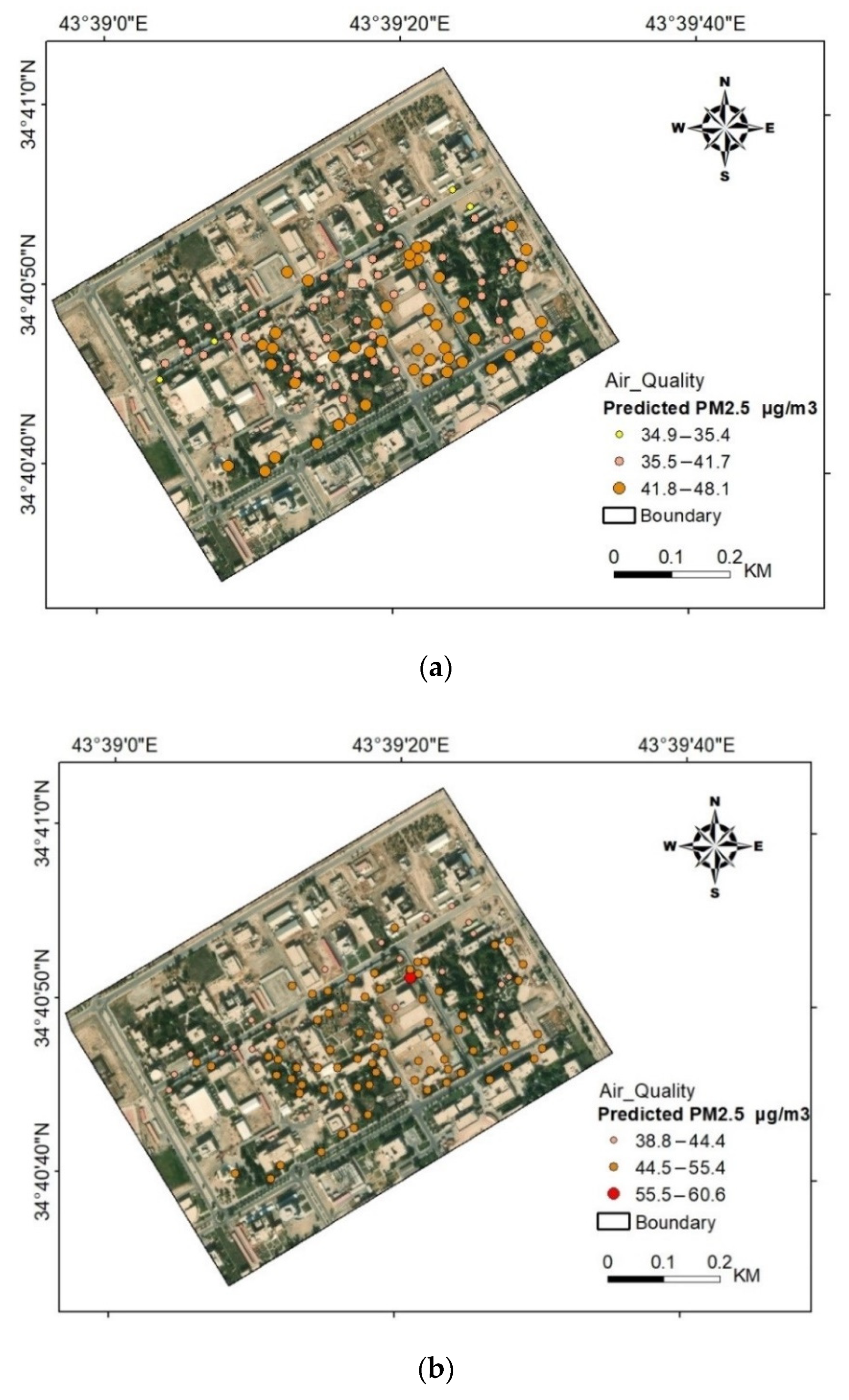
We generated the map for the PM2.5 distribution in the study area and the PM2.5 concentration (as air quality evaluation) was in the range of moderate to unhealthy/harmful.
Figure 3a,b shows the PM2.5 distribution maps in Tikrit University, indicating field dataset values between 35.01 to 58 μg/m
3. Moreover, the satellite imagery distribution validated this dataset, which ranged between 38–58 μg/m
3.
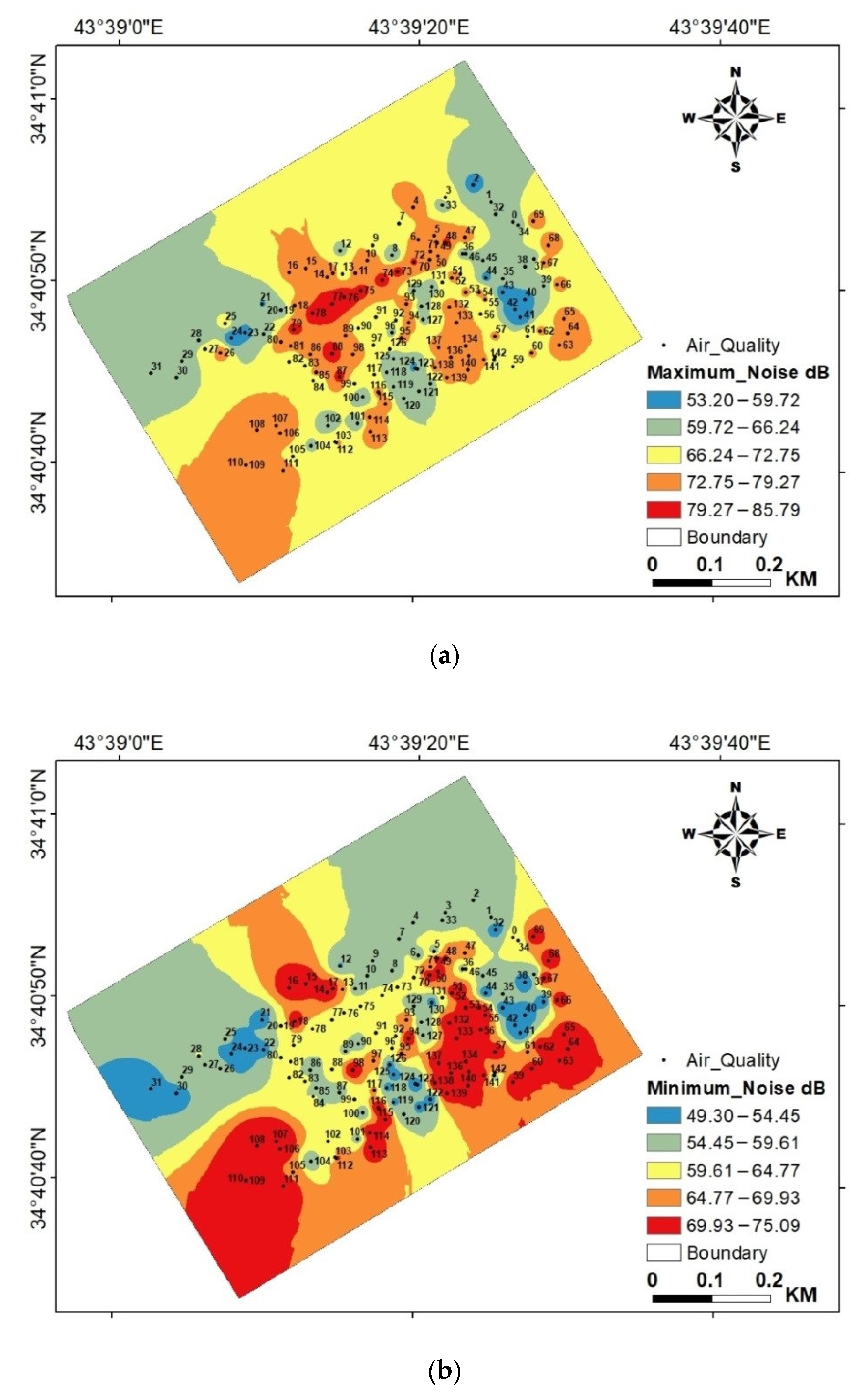
The analyzed noise dataset is subsequently mapped to visualize clusters that exhibit different levels of noise (in dB). Two maps of maximum and minimum noise distributions were produced for Tikrit University, as shown in
Figure 4.
It is important to note that these maps were produced through field measurements at pre-defined sites. Maximum noise levels ranged from 53.20–85.79 dB. In particular, higher maximum noise was observed at location points 48, 76, 77, 78, 79, and 88. Point 48, for example, is near the engineering college laboratories, where loud noise can be due to the electrical generator present in the premises. Points 76 and 77 are near a pharmacy college and a restaurant. Point 78 is located at the sub road between the pharmacy and the science colleges, where a generator set is accompanied by road noise. Points 79 and 88 are near the science colleges. Some collected points are positioned near the abandoned buildings in the university, which might explain why low maximum noise levels were recorded at these locations (i.e., points 41 and 42).
Minimum noise levels were recorded between 49.30 and 75.09 dB. Higher minimum noise levels were recorded at locations 94, 106, 107, and 108. For point 94, the louder minimum noise is due to its location near construction laboratories. Point 106 is on the main road of the university. Point 107 was in the sub-road between the veterinary and science colleges. Point 108 is located near the sports hall and education college lecture rooms. Low minimum noise levels are noticed at points 24, 38, 41,42, 43, and, 44, which were in open space areas and near abandoned buildings.
3.2. Generated Regression Maps
The regression results and model performance are shown in
Figure 5. This figure presents the PM2.5 prediction maps at Tikrit University.
The multiple linear regression model estimates the dependent factor (i.e., PM2.5 particulate mass) from the explanatory variables, in this case: Noise and meteorological parameters. The PM2.5 predicted values ranged between 34.9 and 48.1 μg/m
3 based on 100 measured points in the study area. On the other hand, the predicted PM2.5 values based on satellite imagery ranged between 38.8 and 60.6 μg/m
3.
Table 1 shows the regression statistics and
Table 2 shows the modeling synopsis outputs.
From
Table 1, Multiple R refers to the correlation coefficient of the estimated equation. This output is equal to 0.71 and 0.90 for field dataset and remotely sensed data, respectively. Previous studies indicate that a good correlation has a Multiple R value of 0.70 or greater [
43]. R square (
R2) values are 0.51 and 0.82, respectively for field dataset and remotely sensed data.
R2 refers to the variance ratio for PM2.5, which is explained by the other parameters in the regression equation. In our study, the remotely sensed data show more potential in variance interpretation between variables, where the model correlates PM2.5 to the noise and weather data to predict PM2.5 values in the specified region within the university area. The Adjusted R squared is similar to
R2, but adjusted for the number of predictors in the regression model. The Standard Error is the average estimation error of the model.
One of the synopsis outputs in
Table 2 is the
p-value. In our work, we determined that a variable’s
p-value must not exceed 0.05 or that particular variable will be excluded from the model (i.e., deemed statistically insignificant). As a result, the Noise max variable is not included in the regression equation for the field dataset, as expressed in Equation (3), but included in the equation for the remotely sensed data (Equation (4)). On the other hand, each coefficient isolates the role of the respective variable from all of the other variables. The intercept term is simply the y-intercept where the fitted regression line crosses the
-axis.
is the intercept term,
is the humidity coefficient,
is the temperature coefficient,
is the maximum noise coefficient,
is the minimum noise coefficient, H is humidity, T is temperature,
is the maximum noise, and
is the minimum noise.
3.3. Validation
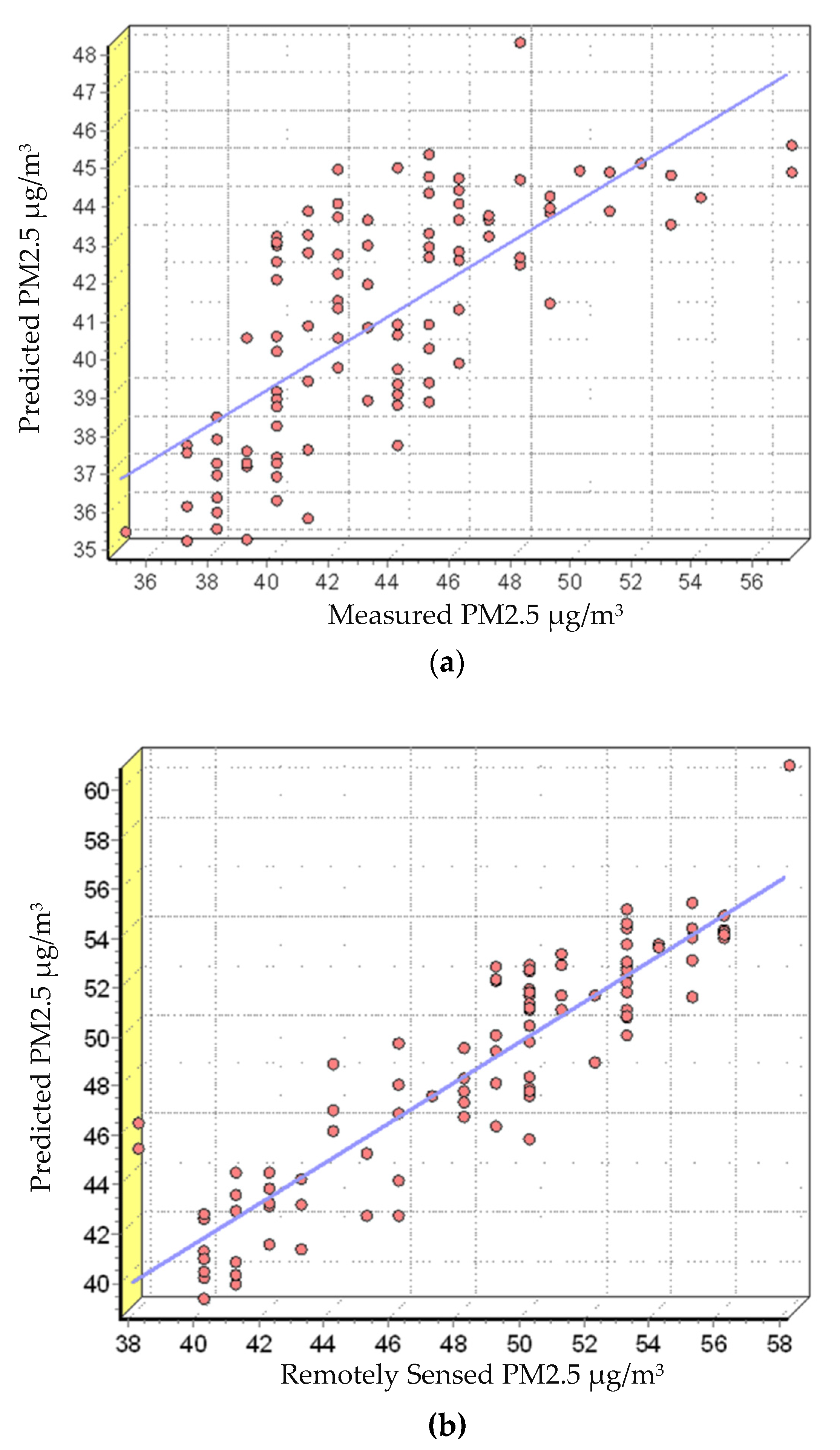
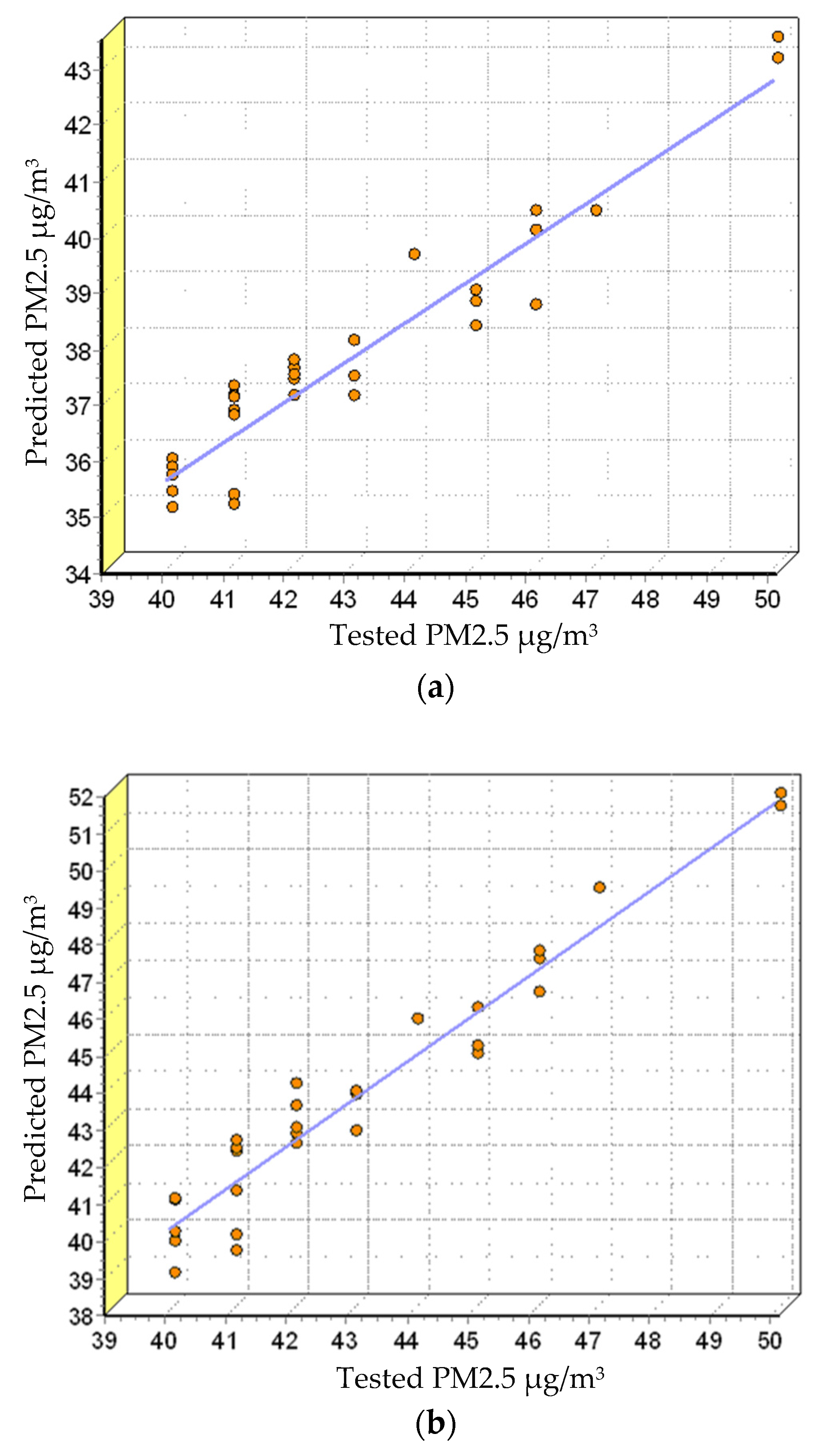
Figure 6a,b shows the linear regression model generated using the field and remotely sensed datasets, respectively. For
Figure 6a, the resultant
R2 based on the field dataset is 0.51. This indicates a low description of the variability, i.e., 51% as the maximum. On the other hand, the
R2 based on remotely sensed dataset is 0.82, indicating a maximum variability description of 82%, which also indicates higher prediction prowess.
3.4. Model Testing
We present the model testing results for both datasets, as shown in
Figure 7.
R2 were 0.91 and 0.94 for the model based on field data and model based on the remotely sensed points, respectively. The results indicate that both models fit the test data well and fall within the confidence range.
4. Discussion
Based on both validated models (
Figure 5a,b), the predicted PM2.5 levels were between 34.9–48.1 μg/m
3 and 38.8–60.6 μg/m
3, respectively. This indicates moderate to harmful air quality (as suggested by the model based on field data) and harmful to unsafe (as suggested by the model based on remotely sensed data). Although both models differed slightly in the predicted values, the air quality seems to be within an unsafe and non-standard safety level, as mentioned in [
44,
45].
The model in
Figure 5a had a low maximum accuracy of 51% obtained by field data fitting. However, increasing the sampling can potentially increase the accuracy. On the other hand, the fitting for the model based on remotely sensed data had a maximum accuracy of 82%. This study tried to attain, at least, a minimum correlation of the noise in the PM2.5 prediction.
The geospatial analysis by GIS technology is one of the important and effective methods for determining emissions of pollutants into the air. At the heart of statistical processes, the regression and estimation models are decision-making tools [
46].
This study also looked at noise pollution. Environmental noise in Tikrit University was measured and then compared with the recommended health standards from WHO.
Figure 4 shows that overall maximum noise levels ranged from 53.20 to 85.79 dB, while minimum noise levels were from 49.30 to 75.09 dB. Note that the WHO guidelines state that noise pollution occurs when levels are above 65 dB [
15]. Moreover, according to [
47], silent zones should not exceed 45 dB. Based on these standards, the results clearly show that the University of Tikrit is categorized as
noisy, which is opposite to what a university should be (i.e., a silent zone). Based on conclusions derived from [
48,
49], university noise levels should be within 35–45 dB. Our findings are crucial as high nose levels can cause non-auditory impacts on students, lecturers, and others alike [
50]. Moreover, this can lead to attention deficits and impaired learning and communication [
51]. The overall outcomes on noise pollution in different areas of Tikrit University indicate that noise levels were high in the different sampling locations. We posit that this was due to the relevant surrounding activities involved, large number of motor vehicles, and the existence of generators.
5. Conclusions
Undoubtedly, air and noise pollution have harmful effects on human health. However, they are unavoidable environmental elements in most urban settings. Researchers are now actively measuring and analyzing both pollutions to gain insight on the causes, as well as to possibly propose solutions where possible. Remotely sensed information and distribution maps can be useful tools for such tasks.
In this paper, air (PM2.5 particulate matter) and noise pollutions are investigated. Specifically, two multiple linear prediction models are generated based on PM2.5 particulate matter measurements and environmental variables (i.e., humidity, temperature, maximum noise, and minimum noise). This study applied the IDW technique and regression analysis based on field measurements and remotely sensed data. Both trained regression models indicate that the PM2.5 particulate and noise pollutions are at undesirable levels in Tikrit University, which could lead to negative consequences if not mitigated. Moreover, and worryingly, this study designated the university as a noisy zone, rather than its supposed designation of being a silent zone.
In terms of the generated linear models, the remotely sensed data-based model had a higher validation accuracy at 82%. Furthermore, model testing showed a 94% accuracy. However, the final prediction values did not differ significantly from the field data-model (at 51% accuracy and 91% testing accuracy).
In conclusion, we believe that mitigative measures can be taken to decrease noise pollutions through planting more trees on both sides of the roads, proper maintenance of the roads, and ensuring that road pavement is based on standard specifications. Moreover, the electrical generators can be covered by silencers to further reduce noise.
Author Contributions
H.J.J. acquired the data; M.H.A. and H.J.J. conceptualized and performed the analysis; M.H.A., A.S.T. and S.J.J. wrote the manuscript, discussion, and analyzed the data; H.J.J., B.K. and N.U. were responsible for supervision and funding acquisition; B.K., N.U. and A.A.H. provided technical sights, as well as edited, restructured, and professionally optimized the manuscript. All authors have read and agreed to the published version of the manuscript.
Funding
This research received no external funding.
Institutional Review Board Statement
Not applicable.
Informed Consent Statement
Not applicable.
Data Availability Statement
Data are available based on request.
Acknowledgments
The authors would like to thank the RIKEN AIP, Japan for providing all facilities during the research.
Conflicts of Interest
The authors declare no conflict of interest.
References
- Bolaño-Truyol, J.; Schneider, I.L.; Cuadro, H.C.; Bolaño-Truyol, J.D.; Oliveira, M.L.S. Estimation of the impact of biomass burning based on regional transport of PM2.5 in the Colombian Caribbean. Geosci. Front. 2021, 101152, in press. [Google Scholar] [CrossRef]
- Somvanshi, S.S.; Vashisht, A.; Chandra, U.; Kaushik, G. Delhi Air Pollution Modeling Using Remote Sensing Technique. Handb. Environ. Mater. Manag. 2019, 1–27. [Google Scholar] [CrossRef]
- Duarte, A.L.; Schneider, I.L.; Artaxo, P.; Oliveira, M.L.S. Spatiotemporal assessment of particulate matter (PM10 and PM2.5) and ozone in a Caribbean urban coastal city. Geosci. Front. 2021, 101168, in press. [Google Scholar] [CrossRef]
- Jumaah, H.J.; Ameen, M.H.; Kalantar, B.; Rizeei, H.M.; Jumaah, S.J. Air quality index prediction using IDW geostatistical technique and OLS-based GIS technique in Kuala Lumpur, Malaysia. Geomat. Nat. Hazards Risk 2019, 10, 2185–2199. [Google Scholar] [CrossRef]
- Huang, K.; Bi, J.; Meng, X.; Geng, G.; Lyapustin, A.; Lane, K.J.; Gu, D.; Kinney, P.L.; Liu, Y. Estimating daily PM2.5 concentrations in New York City at the neighborhood-scale: Implications for integrating non-regulatory measurements. Sci. Total Environ. 2019, 697, 134094. [Google Scholar] [CrossRef] [PubMed]
- Huang, G.; Brown, P.E. Since January 2020 Elsevier Has Created a COVID-19 Resource Centre with Free Information in English and Mandarin on the Novel Coronavirus COVID-19. The COVID-19 Resource Centre Is Hosted on Elsesvier Connect, the Company’s Public News and Information. Available online: https://www.google.com.hk/url?sa=t&rct=j&q=&esrc=s&source=web&cd=&ved=2ahUKEwiykMzcncvyAhUFCqYKHRZNA5AQFnoECAMQAQ&url=https%3A%2F%2Fstacks.cdc.gov%2Fview%2Fcdc%2F87050%2Fcdc_87050_DS1.pdf&usg=AOvVaw0Hl4VYJGwTsEXCu9XpbWI7 (accessed on 20 August 2021).
- Yi, X.; Zhang, J.; Wang, Z.; Li, T.; Zheng, Y. Deep distributed fusion network for air quality prediction. In Proceedings of the 24th ACM SIGKDD International Conference on Knowledge Discovery & Data Mining, London, UK, 19–23 August 2018; pp. 965–973. [Google Scholar] [CrossRef]
- Luo, H.; Guan, Q.; Lin, J.; Wang, Q.; Yang, L.; Tan, Z.; Wang, N. Air pollution characteristics and human health risks in key cities of northwest China. J. Environ. Manag. 2020, 269, 110791. [Google Scholar] [CrossRef] [PubMed]
- Patel, C.J.; Kerr, J.; Thomas, D.C.; Mukherjee, B.; Ritz, B.; Chatterjee, N.; Amos, C.I. Opportunities and challenges for environmental exposure assessment in population-based studies. Cancer Epidemiol. Prev. Biomark. 2017, 26, 1370–1380. [Google Scholar] [CrossRef] [PubMed] [Green Version]
- Jumaah, H.J.; Mansor, S.; Pradhan, B.; Adam, S.N. UAV-based PM2.5 Monitoring for Small-scale Urban Areas. Available online: https://www.researchgate.net/publication/333378629_UAVbasedPM25monitoring_forsmall-scaleurbanareas (accessed on 20 August 2021).
- Zhao, C.; Wang, Q.; Ban, J.; Liu, Z.; Zhang, Y.; Ma, R.; Li, S.; Li, T. Estimating the daily PM2.5 concentration in the Beijing-Tianjin-Hebei region using a random forest model with a 0.01° × 0.01° spatial resolution. Environ. Int. 2020, 134, 105297. [Google Scholar] [CrossRef] [PubMed]
- Hsu, Y.-C.; Chang, S.-H.; Chang, M.B. Efficacy of the novel continuous sampling system for PCDD/Fs and unintentional persistent organic pollutants. Chemosphere 2020, 243, 125443. [Google Scholar] [CrossRef] [PubMed]
- Pérez, P.; Trier, A.; Reyes, J. Prediction of PM2.5 concentrations several hours in advance using neural networks in Santiago, Chile. Atmos. Environ. 2000, 34, 1189–1196. [Google Scholar] [CrossRef]
- Chowdhury, A.K.; Debsarkar, A.; Chakrabarty, S. Novel methods for assessing urban air quality: Combined air and noise pollution approach. J. Atmos. Pollut. 2015, 3, 1–8. [Google Scholar]
- Singh, D.; Kumar, A.; Kumar, K.; Singh, B.; Mina, U.; Singh, B.B.; Jain, V.K. Statistical modeling of O3, NOx, CO, PM2.5, VOCs and noise levels in commercial complex and associated health risk assessment in an academic institution. Sci. Total Environ. 2016, 572, 586–594. [Google Scholar] [CrossRef] [PubMed]
- Munir, S.; Khan, S.; Nazneen, S.; Ahmad, S.S. Temporal and seasonal variations of noise pollution in urban zones: A case study in Pakistan. Environ. Sci. Pollut. Res. 2021, 28, 29581–29589. [Google Scholar] [CrossRef] [PubMed]
- Chandrappa, R.; Das, D.B. Noise Pollution. In Environmental Health-theory and Practice; Springer: Berlin/Heidelberg, Germany, 2021; pp. 141–148. [Google Scholar]
- Ozyavuz, M.; Sisman, E.E. Determination of traffic noise pollution of the city of tekirdag. J. Environ. Prot. Ecol. 2017, 17, 1276–1284. [Google Scholar]
- Wang, L.K.; Pereira, N.C.; Hung, Y.-T. Advanced Air and Noise Pollution Control; Springer: Berlin/Heidelberg, Germany, 2005; ISBN 1592597793. [Google Scholar]
- Murphy, E.; King, E. Environmental Noise Pollution: Noise Mapping, Public Health, and Policy; Newnes: London, UK, 2014; ISBN 0124116140. [Google Scholar]
- Bello, J.P.; Silva, C.; Nov, O.; Dubois, R.L.; Arora, A.; Salamon, J.; Mydlarz, C.; Doraiswamy, H. Sonyc. Commun. ACM 2019, 62, 68–77. [Google Scholar] [CrossRef]
- Di, H.; Liu, X.; Zhang, J.; Tong, Z.; Ji, M.; Li, F.; Feng, T.; Ma, Q. Estimation of the quality of an urban acoustic environment based on traffic noise evaluation models. Appl. Acoust. 2018, 141, 115–124. [Google Scholar] [CrossRef]
- Lagonigro, R.; Martori, J.C.; Apparicio, P. Environmental noise inequity in the city of Barcelona. Transp. Res. Part D Transp. Environ. 2018, 63, 309–319. [Google Scholar] [CrossRef]
- Yang, W.; Park, J.; Cho, M.; Lee, C.; Lee, J.; Lee, C. Environmental health surveillance system for a population using advanced exposure assessment. Toxics 2020, 8, 74. [Google Scholar] [CrossRef]
- Harman, B.I.; Koseoglu, H.; Yigit, C.O. Performance evaluation of IDW, Kriging and multiquadric interpolation methods in producing noise mapping: A case study at the city of Isparta, Turkey. Appl. Acoust. 2016, 112, 147–157. [Google Scholar] [CrossRef]
- Ikechukwu, M.N.; Ebinne, E.; Idorenyin, U.; Raphael, N.I. Accuracy Assessment and Comparative Analysis of IDW, Spline and Kriging in Spatial Interpolation of Landform (Topography): An Experimental Study. J. Geogr. Inf. Syst. 2017, 9, 354–371. [Google Scholar] [CrossRef] [Green Version]
- Fedra, K. GIS and Environmental Modeling. Environ. Model. GIS 1993, 35–50. Available online: http://pure.iiasa.ac.at/id/eprint/3730/1/RR-94-02.pdf (accessed on 20 August 2021).
- Fedra, K. Urban environmental management: Monitoring, GIS, and modeling. Comput. Environ. Urban Syst. 1999, 23, 443–457. [Google Scholar] [CrossRef]
- Kalantar, B.; Ueda, N.; Al-Najjar, H.A.H.; Moayedi, H.; Halin, A.A.; Mansor, S. Uav and lidar image registration: A surf-based approach for ground control points selection. In Proceedings of the International Archives of the Photogrammetry, Remote Sensing and Spatial Information Sciences—ISPRS Archives, Enschede, The Netherlands, 10–14 June 2019; Volume 42. [Google Scholar]
- Ajaj, Q.M.; Shareef, M.A.; Hassan, N.D.; Noori, A.M.; Hasan, S.F. GIS based spatial modeling to mapping and estimation relative risk of different diseases using inverse distance weighting (IDW) interpolation algorithm and evidential belief function (EBF)(Case study: Minor Part of Kirkuk City, Iraq). Int. J. Eng. Technol. 2018, 7, 185–191. [Google Scholar] [CrossRef]
- Kalantar, B.; Ameen, M.H.; Jumaah, H.J.; Jumaah, S.J.; Halin, A.A. Zab River (IRAQ) Sinuosity and Meandering Analysis Based on the Remote Sensing Data. Available online: https://www.researchgate.net/publication/343799487_ZAB_RIVER_IRAQ_SINUOSITY_AND_MEANDERING_ANALYSIS_BASED_ON_THE_REMOTE_SENSING_DATA (accessed on 20 August 2021).
- Al-Najjar, H.A.H.; Kalantar, B.; Pradhan, B.; Saeidi, V.; Halin, A.A.; Ueda, N.; Mansor, S. Land cover classification from fused DSM and UAV images using convolutional neural networks. Remote Sens. 2019, 11, 1461. [Google Scholar] [CrossRef] [Green Version]
- Jebur, A.K. Uses and Applications of Geographic Information Systems. Saudi J. Civ. Eng. 2021, 5, 18–25. [Google Scholar] [CrossRef]
- Sarkar, M.; Das, A.; Mukhopadhyay, S. Assessing the immediate impact of COVID-19 lockdown on the air quality of Kolkata and Howrah, West Bengal, India. Environ. Dev. Sustain. 2021, 23, 8613–8642. [Google Scholar] [CrossRef]
- Stillwell, J.; Clarke, G. Applied GIS and Spatial Analysis; Wiley: Hoboken, NJ, USA, 2006; ISBN 9780470871331. [Google Scholar]
- Hossain, E.; Shariff, M.A.U.; Hossain, M.S.; Andersson, K. A novel deep learning approach to predict air quality index. Adv. Intell. Syst. Comput. 2021, 1309, 367–381. [Google Scholar] [CrossRef]
- Hadi, S.J.; Shafri, H.Z.M.; Mahir, M.D. Factors Affecting the Eco-Environment Identification Through Change Detection Analysis by Using Remote Sensing and GIS: A Case Study of Tikrit, Iraq. Arab. J. Sci. Eng. 2014, 39, 395–405. [Google Scholar] [CrossRef]
- Li, T.; Zhou, X.C.; Ikhumhen, H.O.; Difei, A. Research on the optimization of air quality monitoring station layout based on spatial grid statistical analysis method. Environ. Technol. 2018, 39, 1271–1283. [Google Scholar] [CrossRef] [PubMed]
- Brook, R.J.; Arnold, G.C. Applied Regression Analysis and Experimental Design; CRC Press: Boca Raton, FL, USA, 2018; ISBN 1351465899. [Google Scholar]
- Cook, R.D.; Weisberg, S. Criticism and influence analysis in regression. Sociol. Methodol. 1982, 13, 313–361. [Google Scholar] [CrossRef]
- Weisberg, S. Applied Linear Regression; John Wiley & Sons: Hoboken, NJ, USA, 2005; Volume 528, ISBN 0471704083. [Google Scholar]
- Sen, A.; Srivastava, M. Regression Analysis: Theory, Methods, and Applications; Springer Science & Business Media: Berlin/Heidelberg, Germany, 2012; ISBN 1461244706. [Google Scholar]
- Shareef, M.A.; Toumi, A.; Khenchaf, A. Prediction of water quality parameters from SAR images by using multivariate and texture analysis models. SAR Image Anal. Model. Tech. XIV 2014, 9243, 924319. [Google Scholar] [CrossRef]
- Al-jarakh, T.E.; Hussein, O.A.; Al-azzawi, A.K.; Mosleh, M.F. Design and implementation of IoT based environment pollution monitoring system: A case study of Iraq. IOP Conf. Ser. Mater. Sci. Eng. 2021, 1105, 012037. [Google Scholar] [CrossRef]
- Hamed, H.H.; Jumaah, H.J.; Kalantar, B.; Ueda, N.; Saeidi, V.; Mansor, S.; Khalaf, Z.A. Predicting PM2.5 levels over the north of Iraq using regression analysis and geographical information system (GIS) techniques. Geomat. Nat. Hazards Risk 2021, 12, 1778–1796. [Google Scholar] [CrossRef]
- Caraka, R.E.; Yusra, Y.; Toharudin, T.; Chen, R.C.; Basyuni, M.; Juned, V.; Gio, P.U.; Pardamean, B. Did Noise Pollution Really Improve during COVID-19? Evidence from Taiwan. Sustainability 2021, 13, 5946. [Google Scholar] [CrossRef]
- Chauhan, A.; Pawar, M.; Kumar, D.; Kumar, N.; Kumar, R. Assessment of Noise Level Status in Different Areas of Moradabad City. Researcher 2010, 2, 88–90. [Google Scholar]
- Mahmoud, R.M.; Abbas, A.H.; Yaseen, R.H. Assessment of Noise Pollution and Architectural Solutions for The Colleges and Universities. AUS 2019, 26, 445–453. [Google Scholar]
- Al-Samarrie, M.S.; Mohanad, F.; Salman, A.H. A Study of some Noise Pollution Variables in Sport Halls and Classrooms for College of Sport Education–Tikrit University–Iraq. Int. J. Adv. Sport Sci. Res. 2014, 2, 417–428. [Google Scholar]
- Chijioke, A.M.; Mathias, U.U.; Nwokolo, V.I.; George, I.C. Noise in a Nigerian University. J. Environ. Pollut. Hum. Health 2019, 7, 53–61. [Google Scholar] [CrossRef]
- Ibrahim, S.A. Study Noise Effects on The Students of The Faculty of Engineering/Mustansiriyah University. Al-Nahrain J. Eng. Sci. 2018, 21, 178–186. [Google Scholar]
| Publisher’s Note: MDPI stays neutral with regard to jurisdictional claims in published maps and institutional affiliations. |
© 2021 by the authors. Licensee MDPI, Basel, Switzerland. This article is an open access article distributed under the terms and conditions of the Creative Commons Attribution (CC BY) license (https://creativecommons.org/licenses/by/4.0/).


 ,
, 


