Recharge and Infiltration Mechanisms of Soil Water in the Floodplain Revealed by Water-Stable Isotopes in the Upper Yellow River

Abstract

The stable isotopes (δD and δ¹⁸O) in soil water allow tracing of the flow and transportation of water in the soil. However, there are few studies on the use of soil water stable isotopes to explore the soil water in the floodplain, especially in determining the soil water source and infiltration mechanism. The Bayesian mixing model (MixSIAR) was integrated with the line conditioned excess (lc-excess) of stable isotopes (δD and δ¹⁸O) in precipitation, soil water (0–150 cm), river water, and groundwater to determinate the source and recharge mechanisms of two different soil profile types in the floodplain of the upper Yellow River in Lanzhou, China. The results showed that soil water below 80 cm was affected by river water recharge, affecting soil water content and stable isotopic composition at S1 sampling points (profile parallel to river water); this effect was not observed at S2 (profile is higher than the river water) sampling points. The isotopic compositions of the soil water sources at the two sampling points (S1: δD = −77.41‰, δ¹⁸O = −11.01‰; S2: δD = −74.02‰, δ¹⁸O = −10.56‰) were depleted more than those in the long-term amount-weighted precipitation isotopes (δD = −56.30‰, δ¹⁸O = −8.17‰). The isotope signatures of soil water sources are similar to the isotope characteristics of some high-intensity precipitation events (≥30 mm/day), indicating that soil water originates from a fraction of the total precipitation. The piston flow (60%) and the preferential flow (40%) coexist, but soil moisture and rainfall intensity will affect the sequence of the two infiltration methods. This study provides insights for understanding the hydrological process of the upper Yellow River and evaluating groundwater quality and protecting the floodplain environment.

1. Introduction

As an important part of the water cycle system, soil water connects different hydrological components such as precipitation, surface water, and groundwater [1,2]. Soil water not only determines the water availability for agriculture, but it is also an important factor in soil fertility. It is important for better understanding the soil water transport process, for characterizing the movement of salt, carbon, nitrogen, and other substances, and for increasing the sustainable utilization of water resources [3,4]. Soil water characteristics can be easily modified due to changes in complex factors such as precipitation, evaporation, topography, and vegetation cover. Traditional methods mainly studied the characteristics of water conservancy parameters during infiltration and establish soil water movement models using these parameters. However, it was difficult to explore how the characteristics of soil water changed at different scales [5]. In hydrological research since the 1960s, stable isotope technology has been widely used in the study of water resources. Stable isotopes are very sensitive to evaporation and to precipitation infiltration [6,7], which can result in significant differences in soil water isotope composition at different soil depths. Due to the sensitivity of stable isotopes, it is suitable for describing hydrological processes in a short time [8]. This natural tracer can be used to track information that describes the soil water transport process [9,10].

Hydrologists have long assumed that water flow in the soil is dominated by piston flow (translative and soil matrix flow), where new water entering the soil mixes completely with the existing or resident water, moves deeper into the profile, and ultimately reaches the groundwater and streams. In this process, the new water replaces the old water and pushes it into the deeper layers of soil [11,12]. However, a study of δD-δ¹⁸O revealed that precipitation can quickly reach the deep soil through “fast channels” without mixing with the upper layer of old water [9,13,14,15]. This flow duality is common in the soil hydrological system. Different patterns of precipitation infiltrating into the soil result in different distribution characteristics of soil water isotopes. The transport mechanism of soil water can be described by comparing the isotope characteristics of precipitation and soil water [13,14]. Understanding the mechanism of soil water transport is essential for characterizing the hydrological processes occurring in the soil and how pollutants are transported [16,17].

Many studies have identified the duality of the flow of soil water using the hydrogen and oxygen stable isotope tracer method. For example, Gazis et al. [9] pointed out that if precipitation is in the form of piston flow, “isotopic fronts” after rainfall events with different isotopes will be formed in the soil. The degree of preferential flow depends on soil texture and drainage characteristics. Ma et al. [18] studied a small watershed in a loess hill and gully region, analyzed the stable isotopes of soil water in the unsaturated zone under different land uses during precipitation events, and found that there was a “preferential flow” phenomenon in woodland, grassland, and agricultural land. In addition, grassland and woodland significantly extended the occurrence path of “preferential flow”. Tian et al. [19] studied the stable isotopes of precipitation and soil water in the Naqu area in the central Qinghai–Tibet Plateau and found that during the process of precipitation infiltrating from the surface to the ground, the new water does not completely replace the old water in the soil. This indicates the occurrence of preferential flow, and that the deeper the soil, the more obvious this phenomenon is. Cheng et al. [20] analyzed the stable isotopes in precipitation and soil water of the main land-use types in Changwu County on the Chinese Loess Plateau and found that precipitation is mainly through piston infiltration and that preferential infiltration is not common, which is related to changes in land use. They also found that the possibility of preferential flow occurring was weakened by the deep dry soil layer formed by the negative water balance in high water consumption artificial forest and grass land. Zheng et al. [21] used the traditional method of bright blue solution to study the infiltration mechanism of precipitation in the soil in the Changwu Apple Park. They found that in the apple orchard in the Loess Plateau area where the soil is uniform and affected by mechanical farming, the piston flow is the main mechanism of precipitation infiltration to replenish the soil. Increasing the dumping method can maximize the activation of preferential paths such as macropores. Tan et al. [22] evaluated the mechanism of controlling shallow groundwater recharge in the alpine and hilly areas of the Loess Plateau. In addition to possible vertical slow percolation of soil water through the unsaturated zone, rapid groundwater recharge mechanisms have been identified as temporal preferential infiltration through sinkholes, slip surface, or landslide surface and through the interface of loess layer and palaeo-soils. In addition, many studies have quantified the double-flow mechanism in different regions. For example, Sukhija et al. [23] have quantified these flows at three sites in India with different geological settings and reported the dominance of piston flow in alluvial (100%) and sandstone (68%) aquifers, while the dominance of preferential flow is in a granite aquifer (75%). Manna et al. [24] have also quantified the contribution of piston flow (80%) and preferential flow (20%) in an upland exposed sandstone unsaturated zone from southern California. Although many studies have focused on the characteristics and migration of soil water isotopes in different regions [25,26,27,28], most of these studies focus on artificial experiments under unnatural precipitation or in drier mountainous areas, and the research method is more traditional. There is still limited research on the characteristics of stable isotopes and the mechanism of soil water migration in the floodplain. The Yellow River is the second largest river in China. Located in the land–water crisscross zone, the riparian zone is an important transition zone for the exchange of matter, energy, and information between riverine and terrestrial ecosystems, and is sensitive to changes in the water cycle [29]. Although the changes in soil water movement in the floodplain are very complex and difficult to sample, additional research in this area is essential to improve understanding and potential management practices. In this paper, the stable isotope of hydrogen and oxygen combined with the lc-excess of each water body better reveals the infiltration and replenishment mechanism of the floodplain soil water.

The objectives of this study were to: (1) analyze the characteristics and laws soil water changes on the floodplain of the Lanzhou section of the Yellow River based on soil water content and stable isotopes of soil water hydrogen and oxygen, and (2) based on hydrogen and oxygen isotopic data of various water bodies, lc-excess and the Bayesian framework were used to describe the infiltration mechanism of precipitation in soil. These findings can provide data-based theoretical support for mechanisms impacting the water cycle, for the green construction along the Yellow River, and can improve the understanding of the water cycle in other river basins and similar systems.

2. Materials and Methods

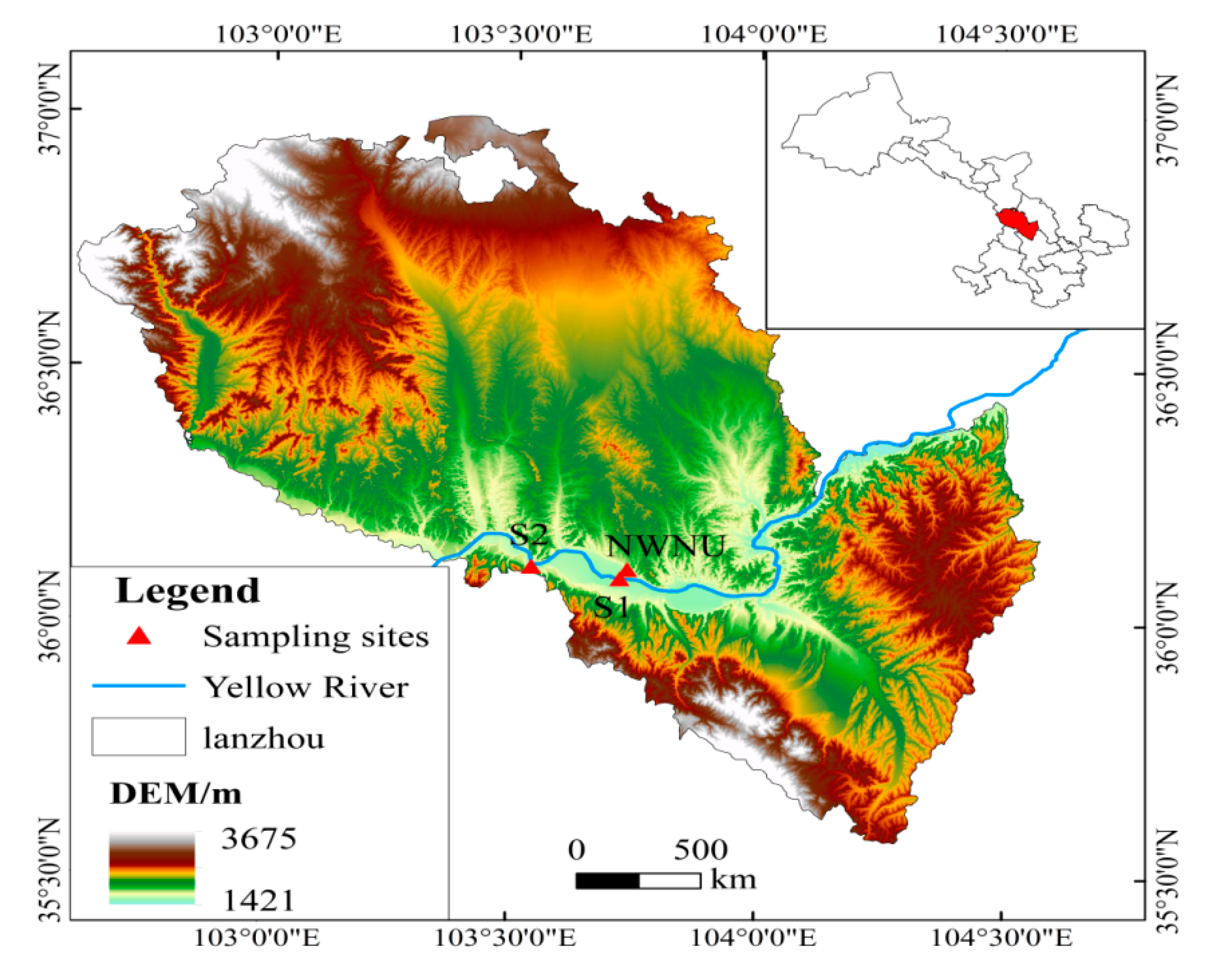
2.1. Study Area

Located in the western Loess Plateau, Lanzhou City (35°53′18″~36°33′56″ N, 103°21′04″~104°00′38″ E) (Figure 1) is in the transition zone of the eastern monsoon region, the high cold region of the Qinghai–Tibet Plateau, and the northwest arid region [30]. Lanzhou is a typical river valley city; the Yellow River runs through the city from west to east, and the southwest region has a higher altitude than the northeast. The altitude of most of the urban areas are between 1500 and 2500 m a.s.l., with beaded valley landforms alternating between canyons and basins [31]. Lanzhou is located in the temperate semi-arid continental monsoon climate zone, with an annual average temperature of 10.3 °C and an annual average precipitation of 324.9 mm, delivered mainly from July to September [31,32]. The Lanzhou section of the Yellow River is 152 km long, 45 km of which flows through urban areas. According to data from the Lanzhou Hydrological Station on the Yellow River, the annual runoff of the mainstream of the Yellow River is 337 × 10⁸ m³, the maximum annual runoff is 511 × 10⁸ m³, and the minimum runoff is 218 × 10⁸ m³. There is a wide floodplain on both sides of the riverbed, which is about 0.5 to 1 km wide, and the high floodplain is about 3 to 4 m above the riverbed. The floodplain is exposed during the dry season and submerged during the flood season, and the soil is composed of coarse silt, fine sand, and very fine sand. The plants on the floodplain mainly include Salix matsudana, Tamarix ramosissima, Ulmus pumila, Phragmites australis, Typha orientalis, Chenopodium glaucum, shamrock Calamari, Calamagrostis pseudophragmites, Polygonum lapathifolium, and Kochia scoparia [32].

2.2. Sample Collection and Processing

From January to November 2019, precipitation was collected on an event basis at the meteorological station of the new campus of Northwest Normal University (Figure 1). A total of 64 daily precipitation samples were collected. Each precipitation sample was collected with a standard funnel rain gauge. In order to avoid the effect of evaporation on precipitation, water samples were collected immediately after each rainfall. The collected samples were stored in 50 mL HDPE plastic bottles, sealed with Parafilm sealing film, and then brought back to the laboratory for preservation in a freezer at −4 °C for isotope analysis. The meteorological data including local precipitation data in 2019 were obtained from the weather query website (https://tianqi.911cha.com/) accessed on 24 July 2021.

Soil samples were collected from two sites (S1 and S2) on the floodplain of the Lanzhou section of the Yellow River at different times in 2019 (Figure 1). S1 (36.09° N, 103.72° E) was near the Jinniu Street Wharf in the Anning District and S2 (36.11° N, 103.54° E) was under the Chaijiaxia Bridge in the Xigu District, Lanzhou City. The distance from S1 to the river is about 10 m, and the surface of the soil is level with the river. The distance from S2 to the river is also 10 m, but the surface layer of soil is 150 cm higher than that of the river. In order to avoid flooding during the flood season, soil samples were collected at S1 from April to June and from August to October 2019, and at S2 from May to October 2019. The sampling frequency was once a month; each sampling was completed between 08:00 and 10:00 local time in order to avoid accelerated evaporation with the increase of temperature. The soil profile from the surface layer to a depth of 150 cm was excavated to obtain soil samples from the floodplain; four soil samples were taken every other 10 cm. Each soil sample was thoroughly mixed manually, then two parts were packed in a sample bottle and sealed with Parafilm for soil water extraction and the other two parts were stored inside aluminum boxes for the determination of the soil water content. Simultaneously, river water and groundwater samples were collected in HDPE plastic bottles sealed with Parafilm and stored at the laboratory in a freezer at −4 °C for isotopic analysis. Six samples were collected for each of the two types.

The collected samples were processed and analyzed in the Stable Isotope Laboratory of the College of Geography and Environmental Science, Northwest Normal University. The detailed processing steps are:

Extraction of soil moisture. The LI-2100 automatic vacuum condensation extraction system (LI-2100, LICA, Beijing, China) was used to extract water from soil samples. The extraction efficiency of the instrument is more than 98%.

Determination of isotopes in water samples. The δ¹⁸O and δD from precipitation, river water, and extracted soil water were measured using a laser spectroscopy liquid water isotope analyzer (T-LWIA-45-EP, ABB-Los Gatos Research, Canada). The abundance of stable hydrogen and oxygen isotopes δ¹⁸O and δD in the measured water samples are expressed in thousandths relative to the Vienna standard average ocean water, V-SMOW:

$$\delta \mathrm{X}=(\frac{R_{\mathrm{sample}}}{R_{\mathrm{standard}}}-1)\times 1000‰$$

(1)

where X is either ¹⁸O or D, R_sample is the ratio of stable isotope abundance in the water sample (²H/¹H or ¹⁸O/¹⁶O), and R_standard is the ratio of stable isotope abundance in standard average ocean water (²H/¹H or ¹⁸O/¹⁶O). The measurement precision is ±0.3‰ for δ¹⁸O and ±1‰ for δD, respectively.

Spectral pollution correction. Studies have shown that the extraction of plants and soil water in the vacuum distillation process may be mixed with methanol and ethanol, which will cause the measurement error from stable isotope infrared spectroscopy to exceed the accuracy of the instrument [33,34,35]. In order to eliminate pollution by methanol and ethanol, spectral analysis software from Los Gatos Research (Los Gatos Research Inc, Mountain View, CA, USA) was used to establish a calibration curve (Figure 2), and then the contaminated data were corrected [36,37].

Soil moisture content determination. The moisture content of the soil was measured using the drying method. Wet soil was weighed with an electronic balance (0.0001 g accuracy), then samples were dried to a constant weight in a constant temperature oven at 150 ± 2 °C and weighed after cooling to room temperature. The weight of the soil, aluminum box, and the soil moisture content (SWC) were calculated as follows:

$$\mathrm{SWC}=\frac{W_1-W_2}{W_2-W_0}\times 100\%$$

(2)

where W₀ is the mass of the aluminum box (g), W₁ is the mass of the aluminum box and wet soil before drying (g), and W₂ is the mass of the aluminum box and dry soil after drying (g).

2.3. Data Analysis

2.3.1. Line-Conditioned Excess

The difference between δD and line-conditioned excess (lc-excess) is the degree of deviation between δD and local meteoric water line (LMWL) in water, which shows the degree of evaporation of different water bodies relative to regional atmospheric precipitation. The lc-excess can better distinguish the different isotopes in precipitation and soil water [38,39,40]. The calculation formula of lc-excess is as follows:

$$\mathrm{lc}-\mathrm{excess}=\delta \mathrm{D}-(\mathrm{a}\times {\delta }^{18}\mathrm{O}+\mathrm{b})$$

(3)

where a and b are the slope and intercept of the LMWL, respectively. δD and δ¹⁸O are the isotope ratios in different water bodies. The average value of lc-excess in precipitation is 0‰. Since the stable isotope fractionation of water from precipitation is affected by evaporation, the lc-excess is usually less than 0‰ [41,42].

2.3.2. Amount-Weighted Precipitation Isotopes

The amount-weighted monthly (or annual) average of ¹⁸O and D in precipitation is calculated as follows:

$$\delta \mathrm{P},\mathrm{mean}=\frac{{\displaystyle \sum _{i=1}^n{\delta }_{p,i}\times PP{T}_i}}{{\displaystyle \sum _{i=1}^{n}PP{T}_i}}$$

(4)

where ${\delta }_{p,i}$ is the δ¹⁸O and δD of the i-th sample, and $PP{T}_i$ represents the precipitation corresponding to the i-th sample.

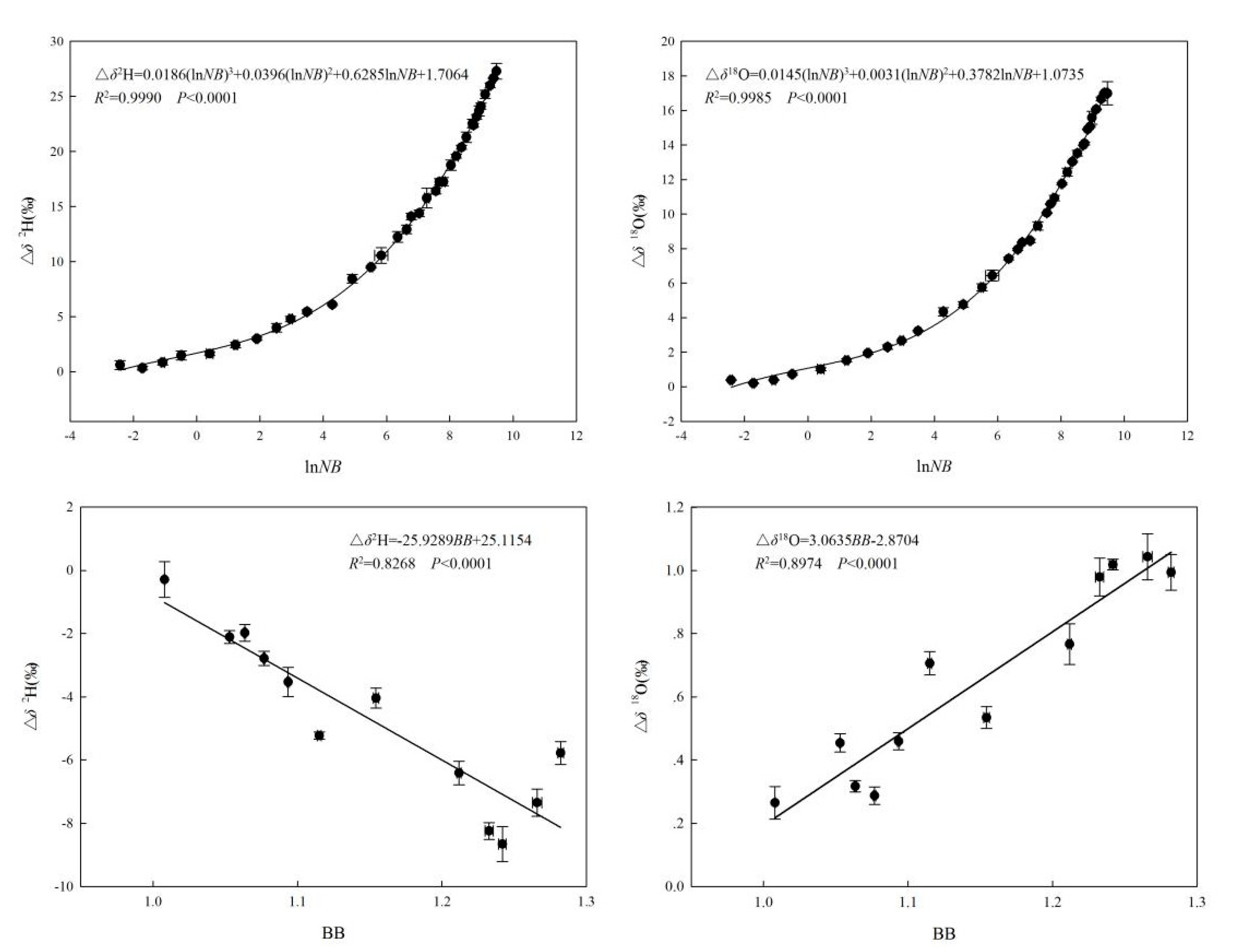
2.3.3. Quantifying Proportions of Dual Flows

The MixSIAR package [43] based on R (R Core Development Team, 2018) was used to quantify the two infiltration mechanisms. The model considers multiple sources, discrimination factors, source values, classification and continuous covariates (random, fixed, classification, nested effects), the uncertainty of prior information, and incorporates the latest results of the Bayesian mixing model.

In this study, only two end members were considered: piston flow and preferential flow. In the framework, stable isotopes in soil water (average and standard error) and precipitation (volume-weighted average and standard error) were used to represent the isotopic features of piston flow and preferential flow, respectively. Groundwater isotopes were considered independent consumers. The discrimination was set to 0 because the stable isotopes of recharging water do not change through both piston and preferential flow [44]. The run length of the Markov chain Monte Carlo (MCMC) was set to ‘long’ (chain length = 300,000; burn = 200,000; thin = 100; chains = 3). It was essential to determine that the model has converged before accepting the output of MixSIAR. We used Gelman–Rubin and Geweke diagnostic tests to determine whether the model has converged. The mean values were presented as the output of the prediction result of MixSIAR.

2.3.4. One-Way ANOVA Analysis

SPSS 16.0 was used to perform single factor analysis of variance (ANOVA) on soil precipitation δ¹⁸O in the wet and dry seasons, soil water content, soil water δ¹⁸O, and lc-excess at different times and locations, and the least significant difference method (LSD) was selected. If p ≥ 0.05, there is no significant difference between the two samples.

3. Results

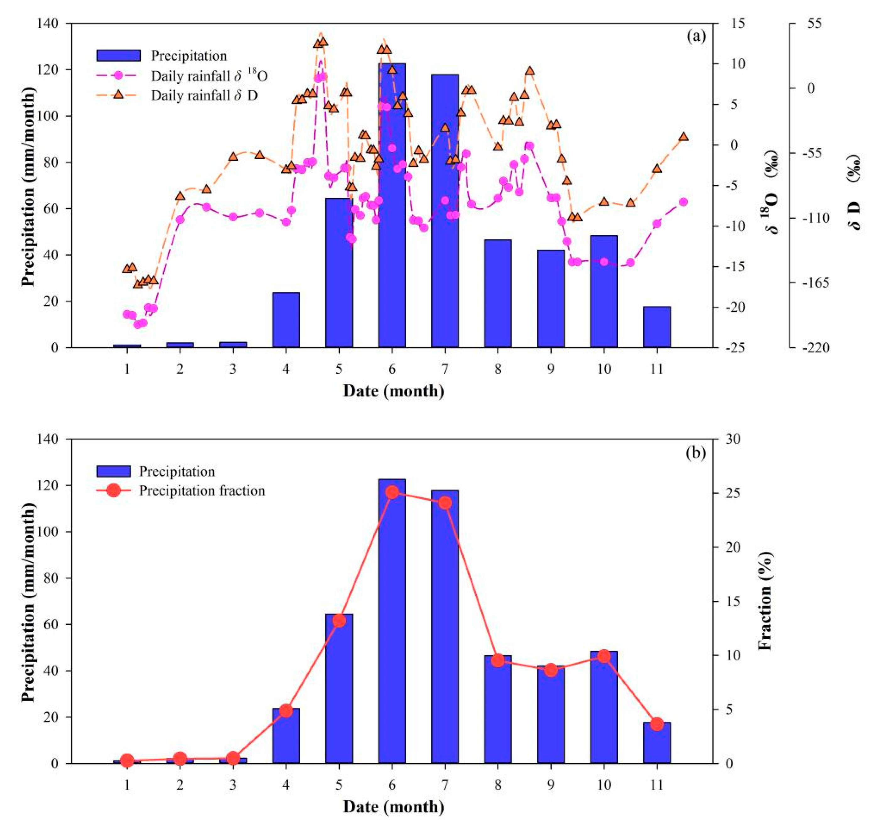
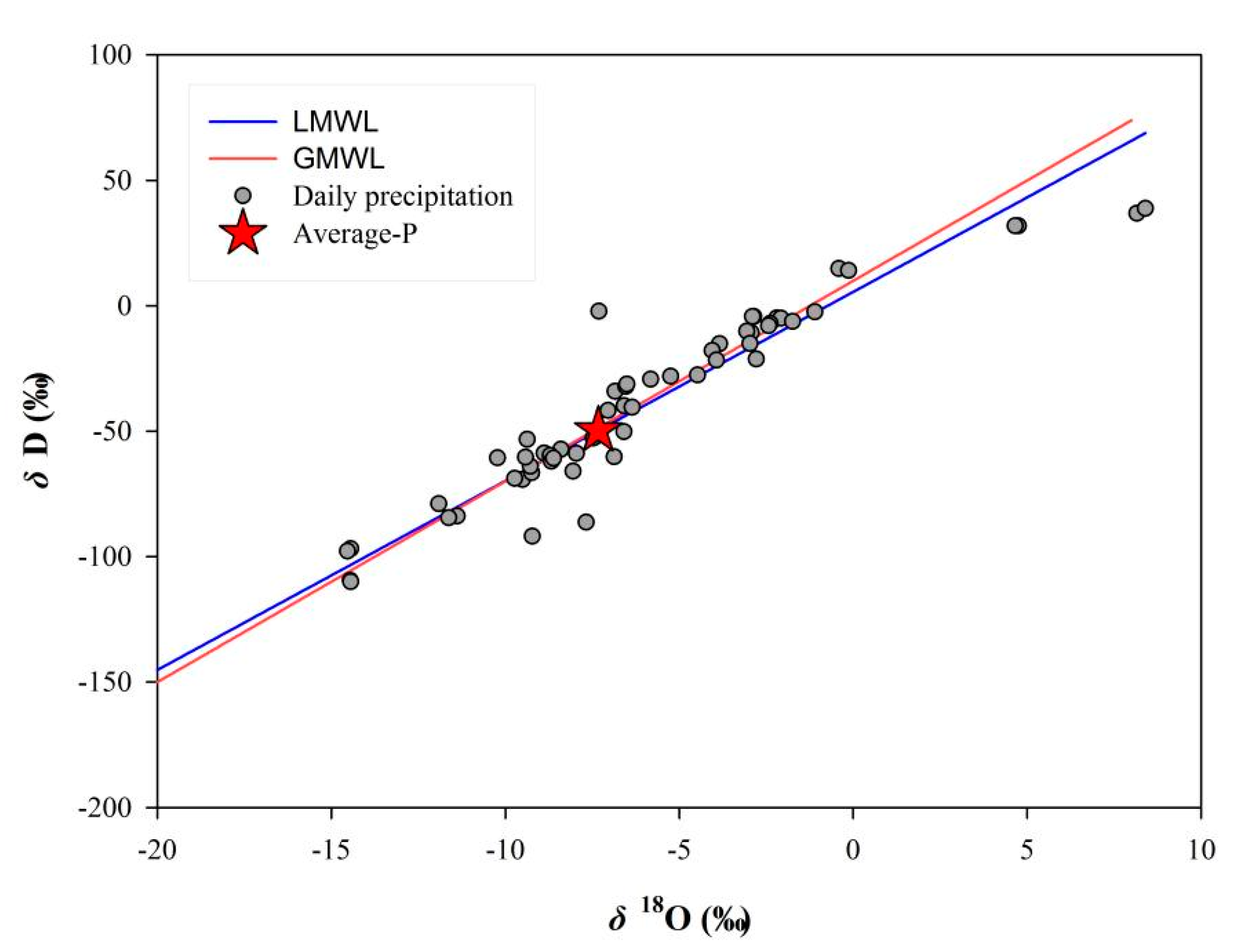
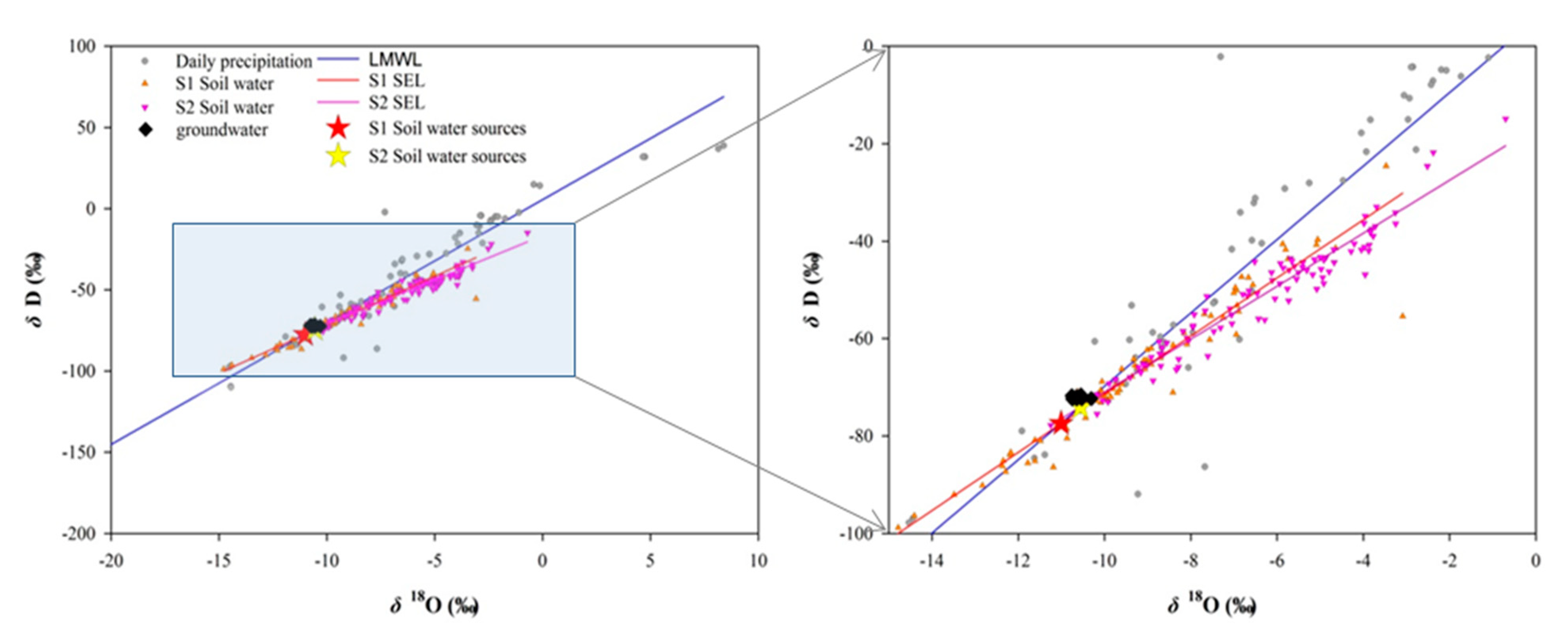
3.1. Stable Isotopic Compositions of Precipitation

The precipitation in the study area in 2019 was concentrated in June and July, with precipitation of 122.6 and 117.8 mm respectively, accounting for 25.08 and 24.09% of the annual precipitation; precipitation from both months accounted for 49.17% of the annual precipitation (Figure 3b). The change in isotope from precipitation during the complete sampling period depended on the precipitation amount. The isotope signature of the whole year revealed that isotopes in the rainy season were more enriched than in the dry season (p < 0.05), showing seasonal variation (Figure 3a). This reflected the large difference in the temporal distribution of precipitation in the study area. The hydrogen and oxygen stable isotope values of 64 precipitation samples were weighed. The weighted average δD and δ¹⁸O of monthly precipitation ranged from −160.73 to −12.74‰ and −21.05 to −3.01‰, respectively; while the annual average was −56.30 ± 43.60‰ and −8.71 ± 5.26‰, respectively. The precipitation in August was the most enriched; the weighted δD and δ¹⁸O were −12.74‰ and −3.01‰, respectively. The most depleted precipitation occurred in January with the weighted δD and δ¹⁸O being −160.73 and −21.05‰, respectively (

Table 1. Monthly precipitation, the proportion of monthly precipitation in total precipitation, and weighted average of stable isotope precipitation in each month; n is the number of samples.

Month	Precipitation (mm)	Fraction (%)	Weighted-δD (‰)	Weighted-δ18O (‰)	n
January	1.2	0.25	−160.73	−21.05	6
February	2.1	0.43	−89.14	−8.45	2
March	2.3	0.47	−57.98	−8.64	2
April	23.7	4.85	−27.55	−4.64	10
May	64.5	13.19	−14.47	−3.30	14
June	122.6	25.08	−24.77	−8.37	7
July	117.8	24.09	−28.93	−5.47	6
August	46.5	9.51	−12.74	−3.01	7
September	42.1	8.61	−64.39	−10.05	6
October	48.4	9.90	−83.34	−14.49	2
November	17.7	3.62	−55.27	−8.39	2

).

Based on the hydrogen and oxygen isotopes in global atmospheric precipitation, Craig [6] proposed the global meteoric water line (GMWL: δD = 8 δ¹⁸O + 10), which represents the average value of global precipitation isotopes. This value has important significance for the study of hydrogen and oxygen stable isotopes in different water bodies and can help guide their use. The local meteoric water line is calculated by the regression line between δD and δ¹⁸O in local daily precipitation (LMWL: δD = 7.54δ¹⁸O + 5.58, R² = 0.94, p < 0.001) (Figure 4). The slope and intercept of the LMWL are both smaller than those of the GMWL, reflecting the climatic characteristics of arid and semi-arid regions with intense evaporation [6].

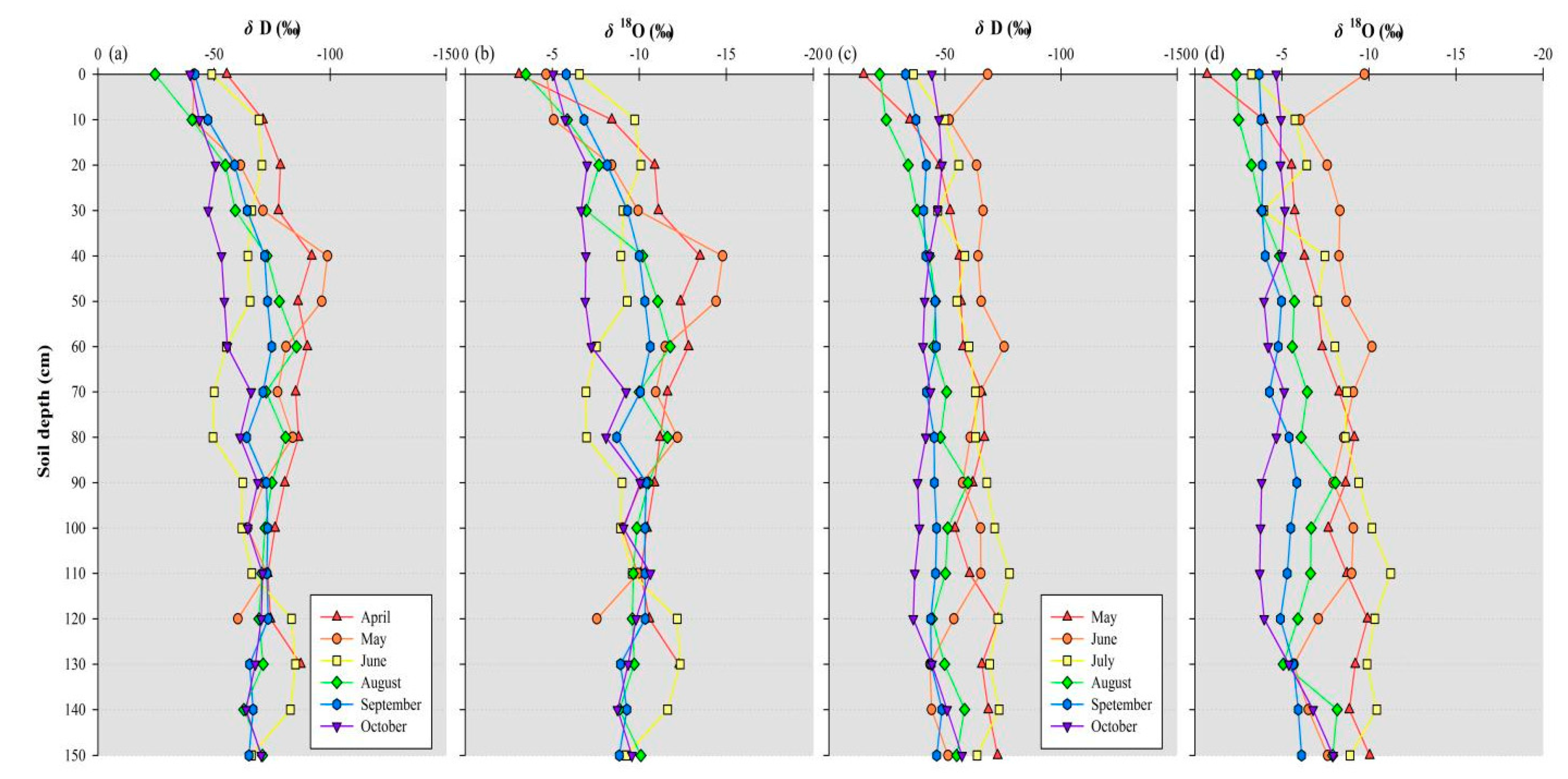
3.2. Stable Isotopic Compositions of Soil Water

Soil water isotope measurements showed that the vertical distribution of soil water isotopes at the two sampling points of the study area was different (p < 0.05). The isotopes from soil water in S1 varied greatly within the range of 0–100 cm, and became relatively stable below 100 cm. The soil water isotopes in S2 were relatively stable over the whole sampling range of the profile, without any obvious changes (Figure 5). The changes of δD and δ¹⁸O in the range of 0–100 cm in S1 were −98.83 to −24.56‰ and −14.78 to −3.09‰, respectively, and those of δD and δ¹⁸O in the range of 100–150 cm were −87.35 to −60.24‰ and −12.35 to −7.56‰, respectively. The δD and δ¹⁸O values from soil water in S2 were −77.78 to −14.88‰ and −11.25 to −0.70‰ in the range of 0–150 cm, respectively. Furthermore, the soil water isotopes at S2 were more enriched than at S1, and the overall variation was smaller. On the time scale, the maximum variation in the vertical distribution of soil water isotopes in S1 (δD: −98.83 to −40.73‰; δ¹⁸O: −14.78 to −4.64‰) and S2 (δD: −72.97 to −14.88‰; δ¹⁸O: −10.04 to −0.70‰) appeared in May. However, the variation of soil water isotopes at the two points in September was the smallest, S1: (δD: −74.86 to −41.72‰; δ¹⁸O: −10.63 to −5.80‰); S2: (δD: −48.71 to −32.98‰; δ¹⁸O: −6.13 to −3.70‰). In addition, at S1, the distribution of soil water isotopes was irregular at different times above 100 cm and gradually converged to one direction below 100 cm, while the vertical distribution of soil water isotopes only showed differences in time at S2.

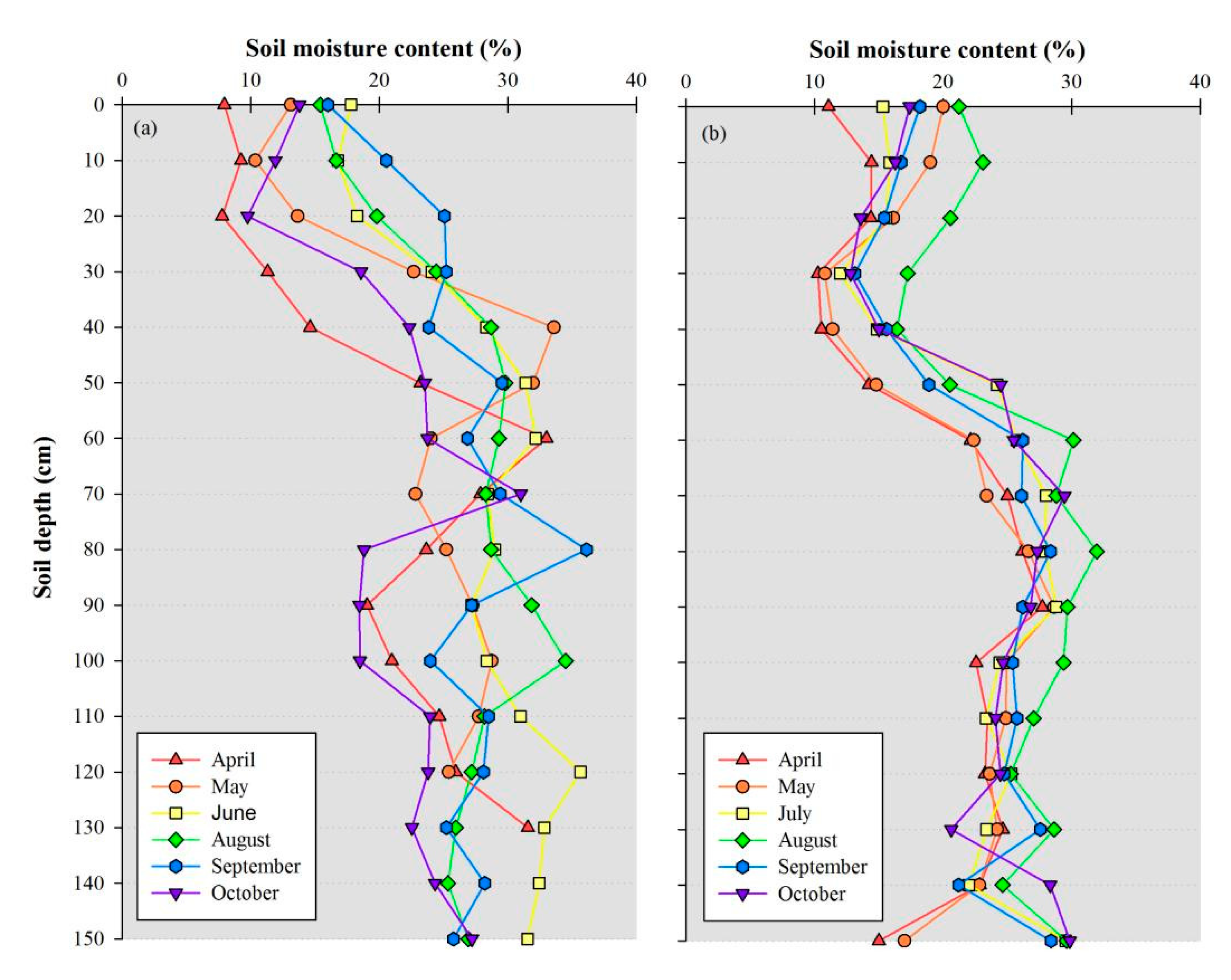
3.3. Soil Moisture Content

According to the measured soil mass water content (Figure 6), the vertical profiles of the soil water content at S1 and S2 showed the same trend of water content increasing with the profile depth, then decreasing after a certain depth (p > 0.05). The difference was that the variation of the range of soil water content at S1 was larger and more complex, and the difference in soil water content at the same depth at different times between the two profiles was clear, and variations in soil water content with depth at the same time step were also very large. However, changes in soil water content in S2 followed a clear rule; the difference of soil water content at the same profile depth at different times was very small, and the variation of soil water content with the same profile depth at the same time was also very small. This phenomenon indicates that the response to precipitation was more obvious at S1 than at S2. The soil water content at S1 varied from 7.76 to 36.10%. The lowest water content was observed at a depth of 0 cm in April and was highest at 80 cm in September. The soil water content at S2 varied from 10.27 to 31.96%. The lowest water content was observed at a depth of 30 cm in May and was highest at 80 cm in August. The lowest water content at both sampling sites occurred at the soil surface before the rainy season, while the highest water content appeared at 80 cm after the rainy season. The high water content areas at both sites were located at depths of 80–100 cm. The soil water content at S2 at 150 cm was higher from July to October than from May to June, indicating that it may be affected by the precipitation during the rainy season.

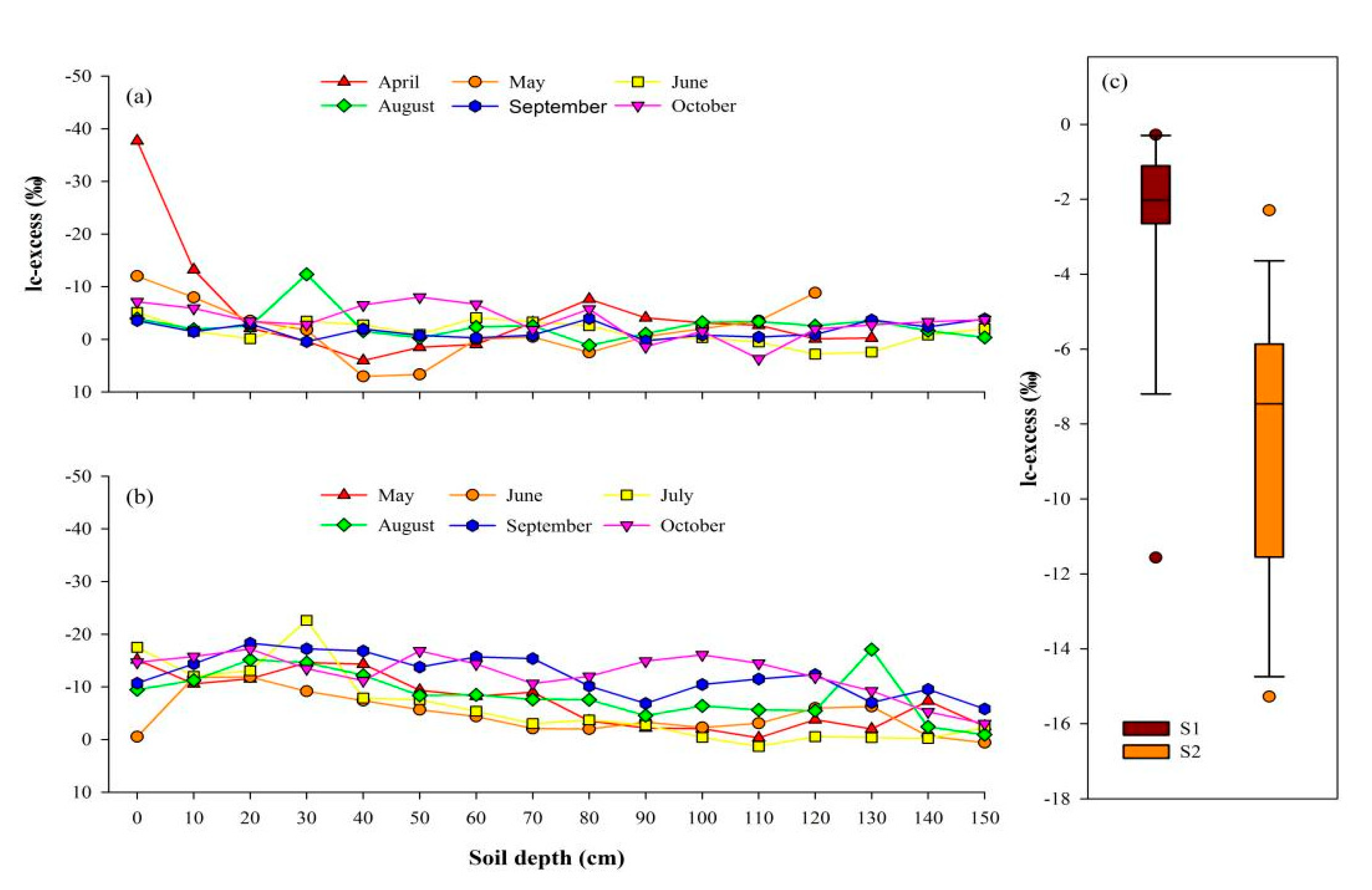
3.4. Lc-Excess of Soil Water

Figure 7 shows the variation of the lc-excess of the water at the two sampling points. The lc-excess at S1 varied from −37.71 to 7.05‰, with an average of −2.58 ±2.69‰. The lowest lc-excess occurred in the soil surface layer (0 cm) before the rainy season; the highest lc-excess occurred at a 40 cm depth in May. The lc-excess at S2 varied from −22.64 to 1.33‰, with the average being −8.57 ± 3.73‰. The lowest lc-excess was observed at a depth of 30 cm in July, while the highest was observed at a depth of 110 cm, also in July. The range of lc-excess values was greater at S1 than at S2, but this change mainly occurred in the surface layer of the soil. When the surface layer was excluded, the change in lc-excess at S1 ranged between −13.21 and 7.05‰. With the exception of the surface layer, there was no significant difference over time in lc-excess values with depth at S1 (p > 0.05). However, at S2 a small difference in lc-excess with time was observed (p < 0.05). During the rainy season, lc-excess was found to be positive as a whole, close to 0‰, while before and after the rainy season it became negative, much lower than 0‰. The average value of soil water lc-excess at different times and for the two sampling sites was calculated according to the profile depth (Figure 7c). It was found that the lc-excess varied less at S1 than at S2 and was closer to the lc-excess value of precipitation (0‰). The lc-excess vertical profile at the two sampling sites decreased with depth as a consequence of the reduction in evaporation of soil water with depth.

3.5. Quantitative Double Flow Mechanism

The soil water at points S1 and S2 was comprehensively analyzed. The annual mean value of soil water isotopes (δD = −59.87‰, δ¹⁸O = −7.94‰), groundwater (δD = −72.10‰, δ¹⁸O = −10.60‰), and precipitation volume-weighted average (δD = −56.41‰, δ¹⁸O = −8.71‰) were used. The relative proportion of piston and preferential flows were quantified using the Bayesian stable isotope mixing model (Figure 8). Overall, piston flow account for 60% ± 26% (average ± SD), and preferential flow account for 40% ± 26%. The difference between the ratio from piston and preferential flow is statistically significant (p < 0.05), further confirming the dominance of piston flow.

4. Discussion

4.1. Comparison of Soil Water Isotope and Soil Water Content

While δD and δ¹⁸O followed the same variation laws, since the molecular weight of D is lower than that of ¹⁸O, the fractionation effect on D was stronger [5]. Therefore, the variation in δD was used to explain the soil water isotope variation with depth. Comparing the changes of soil water isotope and soil water content in S1 (Figure 5a and Figure 6a), the soil water δD within the 0–40 cm layer was found to gradually deplete while the soil water content gradually increased. This was because the soil surface layer is directly affected by evaporation. As water evaporates, the soil water δD in the surface layer became more enriched while the soil water content decreased. Evaporation weakened with depth, leading to more depleted isotope values. On the other hand, the downward infiltration of precipitation without evaporation increased the soil water content. Below 80 cm, the soil water isotope began to become enriched and changed steadily when compared with the 40–80 cm layer, while the soil water content variation at this depth was not obvious. This is similar to the conclusions of Xu et al.’s [45] study on soil slopes in Wolong subalpine dark coniferous forests. The difference is that their study shows that 0–20 cm δD is the smallest, gradually increasing with depth, and tends to be stable below 60 cm. However, this study seems to have reduced the depth by 20 cm. Ma et al. [18] discovered in the central part of the Qinghai–Tibet Plateau that the stable isotopes of hydrogen and oxygen in soil water showed a reverse S-shaped change in the soil profile. This study also found the same change trend.

In general, due to canopy interception and soil evaporation, precipitation infiltrated the soil layer below 80 cm with more difficulty. Due to the specific location of the floodplain and because the soil profile at S1 was level with the river surface, it is possible that the soil water below 80 cm was affected by river water. The average δD of river water was −73.56 ‰, and the average δD of soil water below 80 cm was −71.46 ‰ during the whole sampling period. This result supports that theory. The soil water below 80 cm was recharged by the river and the change in water content was weakened by precipitation maintaining a relatively stable state. At S2, soil water isotopes at the surface layer were the most enriched, except during June, due to evaporation. The lack of soil water isotope enrichment in June may be due to the depletion of soil water isotopes caused by precipitation shortly before sampling. The soil water content was lower from 0–20 cm, then gradually increased with depth (affected by evaporation). Below 80 cm there was a slight decrease, potentially because it is difficult for precipitation to infiltrate into deep soil layers. The results show that S2 (where the soil profile is higher than the river surface) was not affected by the river, excluding the possibility of the river supplying soil water vertically.

4.2. Determination of Soil Water Source

Observations showed that the soil water isotope variation at S1 depended on time and depth, while at S2 it was mostly time-dependent (Figure 5). In the dual isotope space, soil water isotopes of S1 and S2 are plotted closely below the LMWL (Figure 8). Because the LMWL represents the meteoric water inputs to the catchment, calculating the intersection of the SEL and LMWL can trace the isotopic characteristics of the precipitation source [46], while the intersection of SEL and LMWL can determine the isotopic composition of the initial source (Figure 9). The isotopic compositions of the initial sources of soil water at S1 and S2 were (δD = −77.41‰, δ¹⁸O = −11.01‰) and (δD = −74.02‰, δ¹⁸O = −10.56‰), respectively. These values differed slightly, and both were isotopically depleted compared to those of the long-term amount-weighted precipitation (δD = −56.30‰, δ¹⁸O = −8.17‰). When the isotopic signature of soil water sources was compared with that of precipitation, they were similar to those from high intensity precipitation events (≥30 mm/day), indicating that these events contributed to the replenishment of soil water. This phenomenon has also appeared in many previous studies [47,48,49]. Precipitation infiltration is closely related to the rainfall amount and intensity, i.e., the greater the rainfall event, the deeper the rainwater infiltration [50,51]. This could be attributed to the fact that high-intensity rainfall may activate macropores in the soil, enhancing the transfer of permeable water to the deep soil [52].

Soil water isotopes are plotted closely below the LMWL, suggesting soil water had experienced degrees of evaporation. According to this theory-based approach, the isotopic signature from shallow and deep soil water sources were identified, both of which were found to be depleted compared to the isotopic signature of long-term amount-weighted precipitation. This phenomenon can be attributed to the selective infiltration of seasonal precipitation or rainfall events [49]. Therefore, it is probable that soil water recharge came from a part of the total precipitation.

4.3. Soil Water Transport Mode: Preferential Flow and Piston Flow

The two infiltration mechanisms of soil water in floodplain were quantitatively analyzed, and it was found that the piston flow accounted for 60%, and the preferred flow accounted for 40%. Although the piston flow accounted for more, the preferential flow was also obvious, indicating that there was an obvious double infiltration mechanism of soil water in the floodplain. Therefore, we will discuss S1 and S2, respectively, in the following contents.

The soil water δD and δ¹⁸O formed by preferential flow and piston infiltration differ and form an indicative soil water profile that provides an experimental basis for the study of the law of infiltration [9]. The soil profile below 80 cm is greatly affected by the river water recharge, as analyzed above. The soil water isotope signature from depths of 0–80 cm at S1 was discussed. The average values of long-term observations of soil water at S1 (0–80 cm) (δD = −65.22‰, δ¹⁸O = −8.95‰) and S2 (0–150 cm) (δD = −51.80‰, δ¹⁸O = −8.17‰) were compared with the average isotope values of long-term weighted rainfall (δD = −56.30‰, δ¹⁸O = −8.17‰). The isotope from soil water at S1 was closer to that of precipitation (that is, the infiltrated precipitation does not mix too much with the existing soil water), indicating a more preferential flow at S1 than at S2. In addition, a dual-isotope method was used [15], which used lc-excess to identify double flows. The lc-excess method presented advantages over the simpler and more direct analysis of δD and δ¹⁸O that was able to better distinguish the isotopic difference between precipitation and soil water [39]. The long-term observed soil water lc-excess at S1 was closer to that of precipitation (0‰) than that at S2 (Figure 7c), indicating that the degree of isotope fractionation of soil water at S1 was low. This means that precipitation infiltrated the soil mainly in the form of preferential flow. The conclusion obtained by this method is consistent with the above results.

On the other hand, the precipitation with different δD and δ¹⁸O peaks in the piston flow model was retained in the soil profile during the piston flow and gradually disappeared with increasing infiltration depth. In the soil profile at S2, the isotope peak was at 60 cm in June (δD = −75.50‰, δ¹⁸O = −10.17‰), and a similar peak was observed at 110 cm in July (δD = −77.78‰, δ¹⁸O = −11.24‰). This indicates that soil water infiltrated S2 in the form of piston flow. The interval between the two samples was 20 days (from June 27th to July 17th), meaning that the infiltration rate of soil water in the piston flow model of the floodplain soil profile was about 2.5 cm/day. Mali et al. [53] used ¹⁸O isotopes to study the precipitation infiltration process in northern Slovenia by collecting precipitation and soil water at different times at different depths, and calculated the vertical velocity of precipitation infiltration to be 14–15 mm/d. In this study, the reason for the faster infiltration rate of piston flow may be due to the greater soil moisture in the floodplain. Cheng et al. [20] pointed out that when the soil moisture is high and preferential flow occurs under appropriate precipitation conditions, the soil moisture at S1 is affected by river water, while that at S2 is higher than that of the river surface and is not affected by river water, meaning that the soil moisture is less than at S1. This explains why a more preferential flow occurs at S1.

The infiltration pattern of precipitation in the soil profile at two sampling points at different times was observed. It was found that if the surface layer affected by evaporation was excluded, the soil water lc-excess at S1 was closer to the rainfall lc-excess (0 ‰) (Figure 7a) during the months with heavy rainfall (May and June). In addition, S2 manifested the preferential flow signal in precipitation infiltration during this period (May, June, and July), and the lc-excess of soil water below 80 cm was close to that of the rainfall (Figure 7b). These findings suggest that the rainfall amount was among the important causes affecting the infiltration mode of precipitation in the soil. To counter this, soil samples were collected during the early rain period. It was found that if long-term continuous rainfall (rainfall more than 50 mm) or short-term heavy rainfall (intensity > 30 mm/day) occurred before soil samples were collected, these rainfall signals appeared in the deep layer at S2 (>80 cm). The duality of flow is likely ubiquitous in any soil hydrological system [44]. Although clear piston flow signals were observed at S2, preferential flow signals also appeared when there is sufficient rainfall.

4.4. Implications for Environment on Floodplain of the Yellow River

Piston flow is the connected water, but the preferential flow is the disconnected water [54]. Consequently, the proportion of piston flow determines the degree of hydrologic connectivity in the system. The high proportion of piston flow to the total water flow suggested that there was strong connectivity between soil water, river water, and groundwater in the floodplain. Nevertheless, the identified hydrological connectivity here had important implications to water quantity in floodplain. In the process of afforesting the floodplain, some chemical fertilizers will be used, and the solutes of these fertilizers will accumulate in the soil water. This chemical solute can eventually pollute rivers and even groundwater because it can be washed into the groundwater by piston flow, causing the water quality to deteriorate underground. This contamination risk may be reduced by the existence of a preferential flow. Therefore, careful consideration should be given to hydrological connectivity or groundwater recharge mechanisms when assessing the risk of pollutants to floodplain groundwater quality.

5. Conclusions

Stable isotopes (δ²H and δ¹⁸O) of precipitation, soil water, river water, and groundwater were used to determine the replenishment process and infiltration mechanism of soil water in the floodplain of the Lanzhou section of the Yellow River. The results show that the replenishment source of soil water is mainly from high-intensity precipitation (≥30 mm/day), and the river water will replenish the deeper soil water, but it will not replenish upwards. In the study site, the piston flow (60%) and the preferred flow (40%) coexist, but soil moisture and rainfall intensity will obviously cause the sequence of the two infiltration methods. These findings are essential for improving the understanding of the water cycle in other river basins and similar systems.

References

1. Blum, W.E.H. Functions of soil for society and the environment. Rev. Environ. Sci. Bio/Technol. 2005, 4, 75–79. [Google Scholar] [CrossRef]
2. Xu, Y.D.; Wang, J.K.; Gao, X.D.; Zhang, Y.L. Application of hydrogen and oxygen stable isotope techniques on soil water reaearch: A review. J. Soil Water Conserv. 2018, 32, 1–9. (In Chinese) [Google Scholar]
3. Yang, Y.G.; Fu, B.J. Soil water migration in the unsaturated zone of semiarid region in China from isotope evidence. Hydrol. Earth Syst. Sci. 2017, 21, 1757–1767. [Google Scholar] [CrossRef] [Green Version]
4. Evaristo, J.; McDonnell, J.J. Global analysis of streamflow response to forest management. Nature 2019, 570, 455–461. [Google Scholar] [CrossRef]
5. Jin, Y.R.; Lu, K.P.; LI, P.; Wang, Q.; Zhang, T.G.; Liu, Y. Research on soil water movement based on stable isotopes. Acta Pedol. Sin. 2015, 52, 792–801. (In Chinese) [Google Scholar]
6. Craig, H. Isotopic variations in meteoric waters. Science 1961, 133, 1702–1703. [Google Scholar] [CrossRef] [PubMed]
7. Evaristo, J.; McDonnell, J.J.; Scholl, M.A.; Brujinzeel, L.A.; Chun, K.P. Insights into plant water uptake from xylem-water isotope measurements in two tropical catchments with contrasting moisture conditions. Hydrol. Process. 2016, 30, 3210–3227. [Google Scholar] [CrossRef]
8. Stewart, M.K.; Morgenstern, U.; McDonnell, J.J. Truncation of stream residence time: How the use of stable isotopes has skewed our concept of streamwater age and origin. Hydrol. Process. 2010, 24, 1646–1659. [Google Scholar] [CrossRef]
9. Gazis, C.; Feng, X.H. A stable isotope study of soil water: Evidence for mixing and preferential flow paths. Geoderma 2004, 119, 97–111. [Google Scholar] [CrossRef]
10. Deng, W.P.; Yu, X.X.; Jia, G.D.; Li, Y.J.; Liu, Y.J. An analysis of characteristics of hydrogen and oxygen stable isotopes in Jiufeng Mountain areas of Beijing. Adv. Water Sci. 2013, 24, 642–650. (In Chinese) [Google Scholar]
11. Zimmeman, U.; Munnich, K.O.; Roether, W.; Roether, W.; Schubach, K.; Siegel, O. Traces determine movement of soil moisture and evapotrans-piration. Science 1996, 152, 346–347. [Google Scholar] [CrossRef] [PubMed]
12. McDonnell, J.J. The two water worlds hypothesis: Ecohydrological separation of water between streams and trees? Wiley Interdiscip. Rev. Water. 2014, 1, 323–329. [Google Scholar] [CrossRef]
13. Mathieu, R.; Bariac, T. An isotopic study (2H and 18O) of water movements in clayey soils under a semiaridcli-mate. Water Resour. Res. 1996, 32, 779–789. [Google Scholar]
14. Brooks, J.R.; Barnard, H.R.; Coulombe, R.; McDonnell, J.J. Ecohydrologic separation of water between trees and streams in a Mediterranean climate. Nat. Geosci. 2010, 3, 100–104. [Google Scholar] [CrossRef]
15. Evaristo, J.; Jasechko, S.; McDonnell, J.J. Global separation of plant transpiration from groundwater and streamflow. Nature 2015, 525, 91–94. [Google Scholar] [CrossRef] [PubMed]
16. Sprenger, M.; Leistert, H.; Gimbel, K.; Weiler, M. Illuminating hydrological processes at the soil-vegetation-atmosphere interface with water stable isotopes. Rev. Geophys. 2016, 54, 674–704. [Google Scholar] [CrossRef] [Green Version]
17. Brantley, S.L.; McDowell, W.H.; Dietrich, W.E.; White, T.S.; Kumar, P.; Anderson, S.P.; Chorover, J.; Lohse, K.A.; Bales, R.C.; Richter, D.D.; et al. Designing a network of critical zone observatories to explore the living skin of the terrestrial Earth. Earth Surf. Dynam. 2017, 5, 841–860. [Google Scholar] [CrossRef] [Green Version]
18. Ma, J.; Song, W.F.; Wu, J.K.; Wang, Z.J.; Zhang, X.J.; Liu, Z.B. Characteristics of hydrogen and oxygen isotopes of precipitation and soil water in woodland in water source area of yuanyang terrace. J. Soil Water Conserv. 2016, 30, 243–248. [Google Scholar]
19. Tian, L.D.; Yao, T.D.; Tsujmura, M.; Sun, W.Z. Stable isotope in soil water in the middle of tibetan plateau. Acta Pedol. Sinica. 2002, 39, 289–295. (In Chinese) [Google Scholar]
20. Cheng, L.P.; Liu, W.Z. Characteristics of stable isotopes in soil water under several typical land use patterns on Loess Tableland. Chin. J. Appl. Ecol. 2012, 23, 651–658. [Google Scholar]
21. Zheng, S.K.; Si, B.C.; Zhang, Z.Q.; Li, M.; Wu, Q.F. Mechanism of rainfall infiltration in apple orchards on Loess Tableland, China. Chin. J. Appl. Ecol. 2017, 28, 2870–2878. [Google Scholar]
22. Tan, H.B.; Wen, X.W.; Rao, W.B.; Bradd, J.; Huang, J.Z. Temporal variation of stable isotopes in a precipitation-groundwater system: Implications for determining the mechanism of groundwater recharge in high mountain-hills of the Loess Plateau, China. Hydrol. Process. 2016, 30, 1491–1505. [Google Scholar] [CrossRef] [Green Version]
23. Sukhija, B.S.; Reddy, D.V.; Nagabhushanam, P.; Hussain, S. Recharge processes: Piston flow vs. preferential flow in semi-arid aquifers of India. Hydrogeol. J. 2003, 11, 387–395. [Google Scholar] [CrossRef]
24. Manna, F.; Walton, K.M.; Cherry, J.A.; Parker, B.L. Mechanisms of recharge in a fractured porous rock aquifer in a semi-arid region. J. Hydrol. 2017, 555, 869–880. [Google Scholar] [CrossRef]
25. Tian, R.C.; Chen, H.S.; Song, X.F.; Wang, K.L.; Yang, Q.Q. Characteristics of soil water movement using stable isotopes in red soil hilly region of northwest Hunan. Environ. Sci. 2009, 30, 2747–2754. [Google Scholar]
26. Zhang, X.J.; Song, W.F.; Wu, J.K.; Wang, Z.J. Characteristics of hydrogen and oxygen isotopes of soil water in the water source area of Yuangyang terrace. Environ. Sci. 2015, 36, 2102–2108. [Google Scholar]
27. Wang, H.; Li, Z.B.; Ma, B.; Ma, J.Y.; Zhang, L.T. Characteristics of hydrogen and oxygen isotopes in different waters of the Loess hilly and Gully region. J. Soil Water Conserv. 2016, 30, 85–90. (In Chinese) [Google Scholar]
28. Wu, W.; Jiang, W.J.; Jia, Y.N.; Peng, X.Y.; Duan, S.H.; Liu, J.C.; Wang, Z.X. Temporal and spatial distribution of the soil water δD and δ18O in a typical karst vally: A caes study of Zhongliang Mountain, Chongqing city. Environ. Sci. 2018, 39, 5418–5427. [Google Scholar]
29. White, J.C. Water Sources and Ecophysiology of Selected Riparian Species of the Southern Appalachian Mountains. Ph.D. Thesis, Wake Forest University, Winston-Salem, NC, USA, 2015. [Google Scholar]
30. Zhang, L.P. A Syudy of the Human-Environment Relationship in Lanzhou Basin Based on Topography. Master’s Thesis, Lanzhou University, Lanzhou, China, 2017. (In Chinese). [Google Scholar]
31. Zhang, Y.; Zhang, M.J.; Qu, D.Y.; Duan, W.G.; Wang, J.X.; Su, P.Y.; Guo, R. Water Use Strategies of Dominant Species (Caragana korshinskii and Reaumuria soongorica) in Natural Shrubs Based on Stable Isotopes in the Loess Hill, China. Water 2020, 12, 1923. [Google Scholar] [CrossRef]
32. Su, P.Y.; Zhang, M.J.; Qu, D.Y.; Wang, J.X.; Zhang, Y.; Yao, X.Y.; Xiao, H.Y. Contrasting Water Use Strategies of Tamarix ramosissima in Different Habitats in the Northwest of Loess Plateau, China. Water 2020, 12, 2791. [Google Scholar] [CrossRef]
33. West, A.G.; Patrickson, S.J.; Ehleringer, J.R. Water extraction times for plant and soil materials used in stable isotope analysis. Rapid Commun. Mass Spectrom. 2006, 20, 1317–1321. [Google Scholar] [CrossRef]
34. Meng, X.J.; Wen, X.F.; Zhang, X.Y.; Han, J.Y.; Sun, X.M.; Li, X.B. Potential impacts organic contaminant on δ18O andδD in leaf and xylem water detected by isotope ratio infrared spectroscopy. Chin. J. Eco-Agric. 2012, 20, 1359–1365. (In Chinese) [Google Scholar] [CrossRef]
35. Liu, W.R.; Peng, X.h.; Shen, Y.J.; Chen, X.M. Measurements of hydrogen and oxygen isotopes in liquid water by isotope ratio infrared spectroscopy (IRIS) and their spectral contamination corrections. Chin. J. Ecol. 2013, 32, 1181–1186. (In Chinese) [Google Scholar]
36. Schultz, N.M.; Griffis, T.J.; Lee, X.; Baker, J.M. 2011 Identification and correction of spectral contamination in 2H/1H and 18O/16O measured in leaf, stem, and soil water. Rapid Commun. Mass Spectrom. 2011, 25, 3360–3368. [Google Scholar] [CrossRef] [PubMed]
37. Zhao, L.J.; Xiao, H.L.; Zhou, J.; Wang, L.X.; Cheng, G.D.; Zhou, M.X.; Yin, L.; McCabe, M.F. Detailed assessment of isotope ratio infrared spectroscopy and isotope ratio mass spectrometry for the stable isotope analysis of plant and soil waters. Rapid Commun. Mass Spectrom. 2011, 25, 3071–3082. [Google Scholar] [CrossRef]
38. Landwehr, J.M.; Coplen, T.B. Line-Conditioned Excess: A New Method for Characterizing Stable Hydrogen and Oxygen Iso-Tope Ratios in Hydrologic Systems; IAEA: Vienna, Austria, 2006; pp. 132–135. [Google Scholar]
39. Sprenger, M.; Tetzlaff, D.; Soulsby, C. Soil water stable isotopes reveal evaporation dynamics at the soil–plant–atmosphere interface of the critical zone. Hydrol. Earth Syst. Sci. 2017, 21, 3839–3858. [Google Scholar] [CrossRef] [Green Version]
40. Hasselquist, N.J.; Benegas, L.; Roupsard, O.; Malmer, A.; Ilstedt, U. Canopy cover effects on local soil water dynamics in a tropical agroforestry system: Evaporation drives soil water isotopic enrichment. Hydrol. Process. 2018, 32, 994–1004. [Google Scholar] [CrossRef]
41. Sprenger, M.; Tetzlaff, D.; Tunaley, C.; Dick, J.; Soulsby, C. Evaporation fractionation in a peatland drainage network affects stream water isotope composition. Water Resour. Res. 2017, 53, 851–866. [Google Scholar] [CrossRef]
42. Dai, J.J.; Zhang, X.P.; Luo, Z.D.; Wang, R.; Liu, F.J.; He, X.G. 2020 Variation of stable isotopes in soil water Cinnamomum Camphora woods in Changsha and its influencing factors. Acta Pedol. Sin. 2020. [Google Scholar] [CrossRef]
43. Stock, B.C.; Semmens, B.X. MixSIAR GUI User Manual. Version 2013, 3, 1–42. [Google Scholar] [CrossRef]
44. Xiang, W.; Si, B.C.; Biswas, A.; Li, Z. Quantifying dual recharge mechanisms in deep unsaturated zone of Chinese Loess Plateau using stable isotopes. Geoderma 2019, 337, 773–781. [Google Scholar] [CrossRef]
45. Xu, Q.; Liu, S.R.; An, S.Q.; Jiang, Y.X.; Lin, G.H. Characteristics of hydrogen stable isotope in soil water of sub_alpine dark coniferous forest in Wolong, Sichuan province. Sci. Silvae Sin. 2007, 1, 8–14. [Google Scholar]
46. Hervé-Fernández, P.; Oyarzún, C.; Brumbt, C.; Huygens, D.; Bodé, S.; Verhoest, N.E.C.; Boeckx, P. Assessing the ‘two water worlds’ hypothesis and water sources for native and exotic evergreen species in south-central Chile. Hydrol. Process. 2016, 30, 4227–4241. [Google Scholar] [CrossRef]
47. Jasechko, S.; Birks, S.J.; Gleeson, T.; Wada, Y.; Fawcett, P.J.; Sharp, Z.D.; McDonnell, J.J.; Welker, J.M. The pronounced seasonality of global groundwater recharge. Water Resour. Res. 2014, 50, 8845–8867. [Google Scholar] [CrossRef] [Green Version]
48. Li, J.; Pang, Z.; Kong, Y.; Wang, S.; Bai, G.; Zhao, H.; Zhou, D.; Sun, F.; Yang, Z. Groundwater isotopes biased toward heavy rainfall events and implications on the local meteoric water line. J. Geophys. Res. Atmospheres. 2018, 123, 6259–6266. [Google Scholar] [CrossRef]
49. Xiang, W.; Evaristo, J.; Li, Z. Recharge mechanisms of deep soil water revealed by water isotopes in deep loess deposits. Geoderma 2020. [Google Scholar] [CrossRef]
50. Wiekenkamp, I.; Huisman, J.A.; Bogena, H.R.; Lin, H.S.; Vereecken, H. Spatial and temporal occurrence of preferential flow in a forested headwater catchment. J. Hydrol. 2016, 534, 139–149. [Google Scholar] [CrossRef]
51. Jin, Z.; Guo, L.; Lin, H.; Wang, Y.; Yu, Y.; Chu, G.; Zhang, J. Soil moisture response to rainfall on the Chinese Loess Plateau after a long-term vegetation rehabilitation. Hydrol. Process. 2018, 32, 1738–1754. [Google Scholar] [CrossRef]
52. Beven, K.; Germann, P. Macropores and water flow in soils revisited. Water Resour. Res. 2013, 49, 3071–3092. [Google Scholar] [CrossRef] [Green Version]
53. Mali, N.; Urbanc, J. Isotope oxygen-18 as natural tracer of water movement in a coarse gravel unsaturated zone. Water Air Soil Pollut. 2009, 203, 291–303. [Google Scholar] [CrossRef]
54. Good, S.P.; Noone, D.; Bowen, G. Hydrologic connectivity constrains partitioning of global terrestrial water fluxes. Science 2015, 349, 175–177. [Google Scholar] [CrossRef] [PubMed] [Green Version]
Figure 1. The geographical location of the Lanzhou section of the Yellow River and soil sampling points and the meteorological station of Northwest Normal University (NWNU).
Sustainability 13 09369 g001
Figure 2. Relationship between the lnNB and offset in δ2H and δ18O and relationship between the BB and offset in δ2H and δ18O.
Sustainability 13 09369 g002
Figure 3. Monthly precipitation and δD and δ18O of daily precipitation (a), and monthly precipitation and the proportion of monthly precipitation to total precipitation during the sampling period (b). The blue column in (a) represents the monthly precipitation, and the dashed line with circle and dashed line with triangular represent the δD and δ18O of precipitation respectively.
Sustainability 13 09369 g003
Figure 4. Dual-isotope plots precipitation. The GMWL and LMWL respectively represent the global meteoric water line (δD = 8 δ18O + 10) and the local meteoric water line (δD = 7.54δ18O + 5.58, R2 = 0.94, p < 0.001). The red star is the average of all precipitation samples during the sampling period (δD = −49.65‰, δ18O = −7.33‰).
Sustainability 13 09369 g004
Figure 5. The variation characteristics of soil water δD and δ18O at different depths in S1 (a,b) and S2 soil profiles during the sampling period (c,d).
Sustainability 13 09369 g005
Figure 6. Variation characteristics of soil water content at different depths at soil profile S1 (a) and S2 (b) during the sampling period.
Sustainability 13 09369 g006
Figure 7. (a,b) represent the lc-excess values of soil water at different soil depths at sampling points S1 (a) and S2 (b), respectively, during the sampling period. The box plot (10th, 25th, 50th, 75th, and 90th) of soil water lc-excess is shown in (c).
Sustainability 13 09369 g007
Figure 8. Isotope-based estimation of relative proportion for piston and preferential flows using the Bayesian mixing model (MixSIAR).
Sustainability 13 09369 g008
Figure 9. Dual-isotope plots precipitation, soil water, and groundwater. The brown and purple lines are the soil evaporation lines (SEL) at S1 and S2 based on soil water isotopes, (S1: δD = 5.97δ18O−11.70; S2: δD = 5.44δ18O−16.59). Red and yellow stars represent the S1 and S2 soil source water values, respectively.
Sustainability 13 09369 g009