1. Introduction
Rail transit tunnels have a large span and pass through a variety of complex geological environments. The geological variability may induce differential structural settlement, resulting in track damage and reducing the service life of rail transit-related facilities. In addition, it may cause structural damage to tunnels and eventually lead to accidents in urban rail transit operation. Therefore, it is of great significance to monitor and diagnose uneven structural settlement in rail transit tunnels with monitoring data [
1].
Traditionally, the uneven settlement monitoring of rail transit tunnels is mainly based on manual measurement with surveying and mapping instruments, which require considerable manpower and material resources. This approach cannot be used to achieve long-term automatic monitoring. An electronic level, which can be operated for a long period, was developed; however, it has a high price and short service life [
2,
3,
4]. With the development of advanced sensing technology, distributed fiber sensors have provided a new method [
5] of monitoring the uneven settlement of rail transit tunnels, especially methods based on Brillouin scattering [
6,
7,
8,
9,
10], including Brillouin optical time domain analysis (BOTDA) and Brillouin optical time domain reflectometry (BOTDR).
Recently, the development of AI technology and the technical progress of structural health monitoring [
11,
12] have provided strong support for the diagnosis of the damage of civil structures, and many researchers have focused on the structural health monitoring of tunnels, providing theoretical support for the diagnosis of uneven settlement. Li [
13] designed an automatic monitoring system with a static level to monitor the settlement of tunnels. Shi [
14] adopted BOTDR technology to monitor the strain and temperature in the Nanjing Gulou tunnel. Shen [
15] proposed a monitoring strategy to monitor distributed settlement in shield tunnels by combining quasi-distributed fiber Bragg grating sensors with a hydrostatic level measuring system. Zhang [
16] took advantage of manual and automatic methods to perform deformation monitoring of tunnels, in which the manual monitoring relied on a level and total station, while the automatic monitoring relied on a laser rangefinder and static leveling system. Liu [
17] proposed a method for detecting the structural damage of operating tunnel by using the high-density cross-sectional curvature. With the development of artificial intelligence (AI) technology, great progress has been made in the field of tunnel construction and structural monitoring. AI technology, e.g., support vector regression (SVR) [
18] and gene expression programming (GEP) models [
19,
20,
21], were applied to predict the performance of tunnel boring machines (TBM). To solve the problems of ‘clogging’ and disc cutter consumption in tunnel excavation, AI algorithms such as neural networks and genetic algorithms were implemented to assess the tendency for clogging and estimate the disc cutter life [
22,
23]. Computer vision-based technology was provided to monitor the activities of tunnel construction [
24]. Among AI methods, SVM is an intelligent algorithm with high efficiency, and it has been widely used in ground vibration prediction [
25], rock brittleness prediction [
26], predicting the strength of fiber-reinforced cement paste backfill [
27] and identifying changes in soil type during tunnelling [
28]. Thus, in this study, the SVM algorithm is utilized to diagnose the uneven settlement of tunnels.
Specifically, there has been a considerable amount of research focused on the uneven settlement of tunnels. Mair [
29] found that the settlement displacement during an operation period was far greater than that caused by construction after the long-term monitoring period, which shows that uneven settlement is one of the main structural issues of tunnels. Attewell [
30] found, by collecting and analyzing a considerable amount of monitoring data, that the long-term settlement of tunnels was significantly affected by the upper layer soil. Ranjith [
31] proposed an empirical formula for tunnel settlement based on the settlement trend of tunnels in soft soil. Wang [
32] investigated the influence of uneven settlement on tunnel linings and longitudinal anchors.
In recent years, research on the mechanism of the uneven settlement of tunnels has been popular, but research on the monitoring-data-based diagnosis of the uneven settlement of tunnels is still lacking. In this study, the distributed optical fiber sensing technology is implemented to obtain a massive amount of strain data from densely distributed measurement points along regional railway tunnels. Using the data provided by the distributed optical sensing fiber, an algorithm for diagnosing the uneven settlement of regional railway tunnels based on the spatial correlation of high-density strain measurement points is proposed. The high-density strain measurement points provide more information of tunnel deformation than the regular way; thus, it is more prone to detect the occurrence of the uneven settlement of a tunnel. The proposed method is a new investigation on how to utilize the monitoring strain data obtained from high-density strain measurement points to diagnose the potential risk of uneven settlement of long-distance rail transit tunnels.
The outline of this paper is organized as follows: first, the distributed strain measurement principle based on BOTDA is introduced; second, a support vector machine (SVM)-based method for determining the zone of a tunnel possessing high spatial correlation between different strain measurement points is proposed; third, the method of diagnosing the uneven settlement of a tunnel by using the spatial correlation between strain measurement points is proposed; and finally, the effectiveness of the proposed method is verified through numerical examples and actual monitoring data. At the end of this paper, the conclusions are summarized.
2. Strain Measurements Obtained from BOTDA Sensors
Distributed fiber sensing technology based on Brillouin scattering has the advantages of a long monitoring distance and high spatial resolution and thus has promising prospects in tunnel monitoring. Brillouin scattering-based fiber sensing technology can be briefly divided into two types: BOTDA and BOTDR. Compared to BOTDR, BOTDA provides a higher spatial resolution and better data accuracy, which is more suitable for structural monitoring with a high density of strain measuring points.
The structural strain and ambient temperature will lead to the Brillouin frequency shift of the fiber sensor; conversely, the structural strain and ambient temperature can be obtained by analyzing the Brillouin frequency shift [
33,
34], which can be calculated as follows:
where
n refers to the refractive index of the fiber sensor,
is the light wave velocity and
is the wavelength of incident light. The light wave velocity
can be obtained as follows:
where
,
E and
are Poisson’s ratio, Young’s modulus and the density, respectively.
Structural strain and environmental temperature can affect the refractive index of the fiber sensor pasted on the tunnel structure according to the elasto-optic and thermo-optic effects, thus changing the Brillouin scattering frequency shift, which has a linear relation with structural strain and environmental temperature, as shown below:
where
Cv,T and
denote the temperature and strain effect factors, respectively, which can be determined by constant temperature and pressure experiments.
In practical application, temperature compensation is set to eliminate the environmental effect on the Brillouin scattering frequency shift to measure the real structural strain. Furthermore, for the monitoring of urban rail transit structures, a distributed fiber sensor is installed along the monitored tunnel, and then a massive amount of strain data is collected from high-density measurement points during long-term monitoring, which addresses the disadvantages of traditional point sensors such as their inconvenient installation and high price. In summary, the advanced sensing technique provides a data foundation for the uneven settlement diagnosis of rail transit tunnels.
3. SVM-Based Method for Determining the Zone of a Tunnel Possessing a High Spatial Correlation between Different Strain Measurement Points
Long-distance tunnels usually pass through areas with different geological conditions, leading to different structural forms, design approaches and construction methods; thus, the spatial correlations between strain measurement points in different regions may vary greatly. Therefore, it is necessary to divide the whole rail line into different zones according to the similarity of the spatial correlations between strain measurement points at the beginning of the diagnosis process of the uneven settlement of rail transit tunnels.
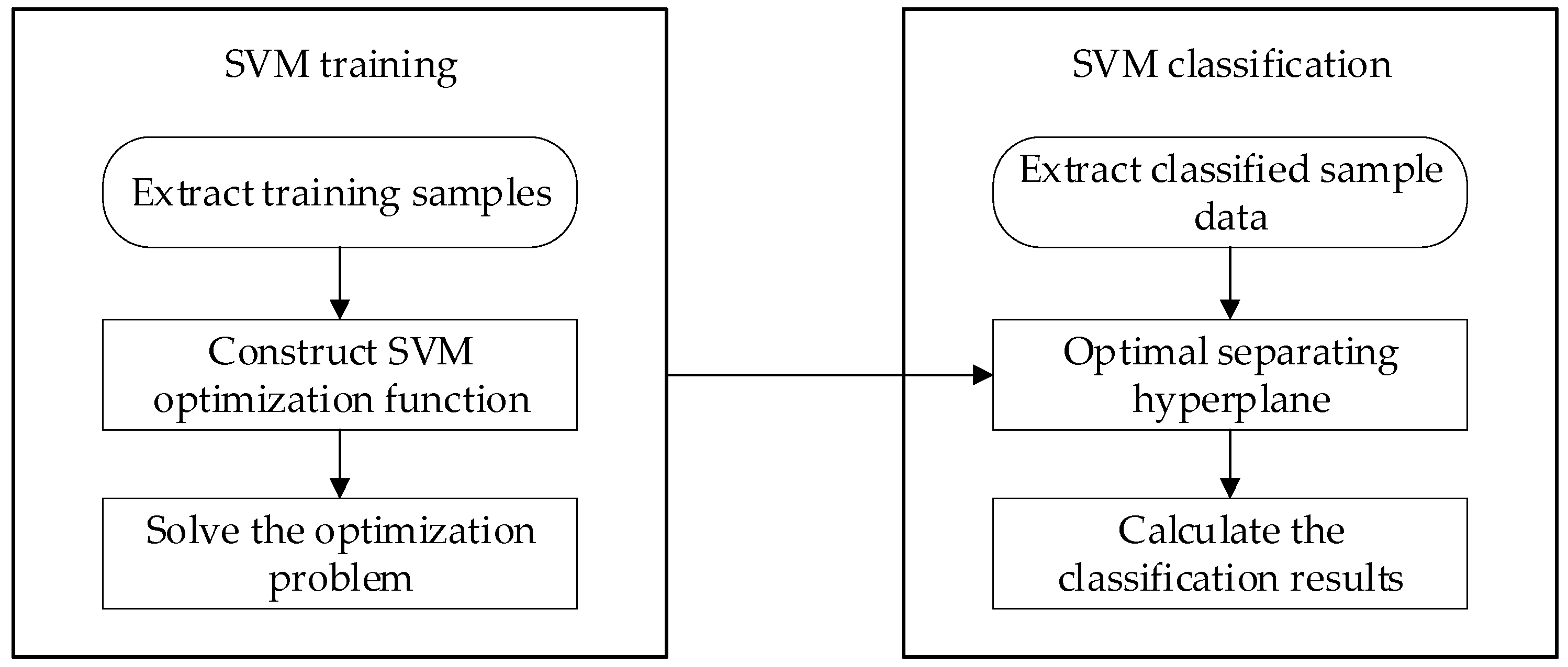
SVMs have unique advantages in dealing with classification problems, such as clear principles, simple methods and convenient operations. In this paper, the SVM technique is selected to perform cluster analysis on strain monitoring data. The approach used to determine tunnel zones with a high spatial correlation among the corresponding strain measurement points is shown as follows [
35]:
For the sample classification problem, assuming that the sample data are
x, the final classified category is
y (including 1 and −1); thus, the separating hyperplane can be expressed as a decision boundary as follows:
where
w and
b are the normal vector and intercept of the separating hyperplane, respectively, and the distance from a random data point to the separating hyperplane is shown as:
Normalizing
w and
b results in the following:
where
denotes to the norm of a vector.
The farther the distance from the data point to the separating hyperplane is, the more reliable the data classification will be; thus, the objective function can be described as .
Additionally, the constraint condition of the data classification can be expressed as follows: (1) all sample data are classified correctly; (2) the separating hyperplane should coincide with the central axes of the final two classified sample data, which can be expressed as follows:
Hence, the objective function can be given as:
We find that the objective function
is equal to
; thus, Equation (8) can be switched into a Lagrangian formulation of the problem, as shown below:
Thus, the objective function can be described as:
The above equation can be dualized to Equation (12):
To solve the classification hyperplane equation, we take the derivatives of Equation (9) with respect to
w and
to obtain:
Substituting Equation (13) into Equation (9), we can obtain the solution as follows:
Then, the maximum value of α can be obtained as:
Through the above process, we can obtain the solutions of , w and b and ultimately identify the separating hyperplane.
For high-density strain monitoring data of rail transit tunnels, assuming that there are m types of data categories in the data samples, we can obtain a separating hyperplane between every two types of data categories, with
m(
m − 1)/2 separating hyperplanes in total. Using the obtained hyperplanes, the monitoring data can be classified to determine the zones of the tunnel possessing high spatial correlations among the corresponding strain measurement points, and the SVM classification procedures are shown in
Figure 1.
4. Method of Diagnosing the Uneven Settlement of Tunnels by Using the Spatial Correlation between Strain Measurement Points
For tunnel zones with a high spatial correlation between different strain measurement points, to diagnose the uneven settlement of tunnel zones among points with similar strain data, a method based on the spatial correlation between strain measurement points is proposed. First, the classified tunnel zones are precisely redivided into various sections according to the influence range of the uneven settlement, and the vector angles between adjacent strain measuring sections are calculated. Second, the diagnosis threshold of uneven settlement is constructed with the acquired vectorial angles under healthy conditions. Finally, the diagnosis factor is calculated with the structural strain data obtained during the tunnel operation, with which the uneven settlement of the rail transit tunnel is detected.
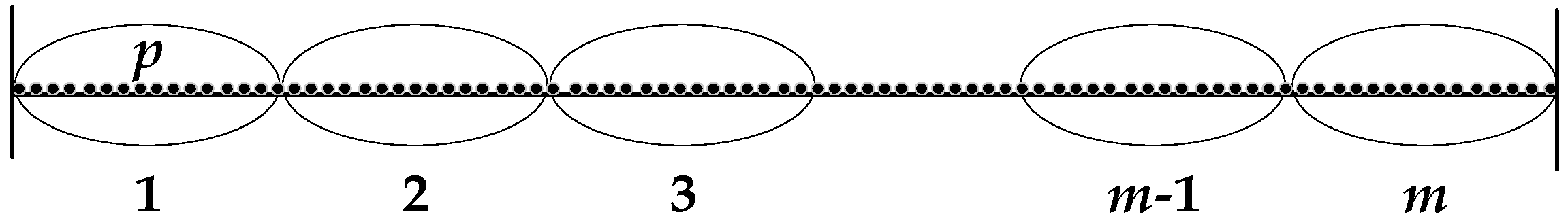
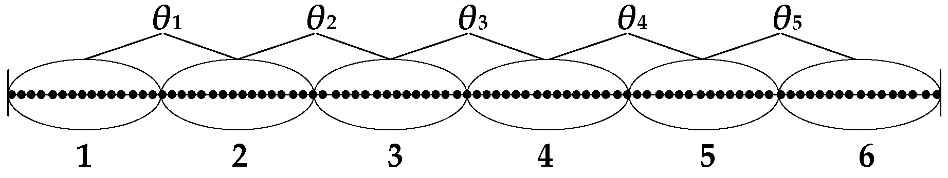
To further divide the tunnel zones with similar strain data into various sections and determine the length of the corresponding sections, numerical simulation can be undertaken to calculate the influence ranges under different uneven settlement conditions. Along the calculated length, each tunnel zone is divided into
m parts, and every part contains
p measuring points. The tunnel structure section distribution for a single data category is displayed in
Figure 2.
The strain monitoring data of each section are formed into a vector, and then
m vectors can be obtained in a tunnel zone, expressed as
x1,
x2, K,
xm. The angles of the strain monitoring vectors between adjacent sections are calculated as follows:
The angles in one tunnel section at a certain moment can be denoted as
, which can be combined into a data set, as shown below:
Then, the data sets of all the adjacent sections in one tunnel zone can be assembled as:
For each data set of strain vector angles between adjacent sections, the mean value and covariance matrix can be calculated as follows:
With Equations (19) and (20), we can obtain the Mahalanobis distance of each data set:
The Mahalanobis distance calculated with Equation (21) can be regarded as the diagnosis factor for the uneven settlement of the rail transit tunnel; then, we can obtain the diagnosis factors of
n different times in the reference state:
Similarly, the diagnosis factors between all the adjacent sections under the same category can be calculated and formed into one matrix:
For each diagnosis factor vector, we can sort the
n elements of the vector from the smallest to the largest, as shown below:
where
and
are the smallest and largest elements in vector
Di, respectively, and we can use the 95% confidence interval to obtain the diagnosis threshold of uneven settlement
. To increase the effectiveness of this threshold, a coefficient
(larger than 1) is introduced, and the modified threshold can be expressed as:
All the diagnosis thresholds between all adjacent sections under the same category can be obtained using the above process, as shown in Equation (26):
The next step of diagnosing uneven settlement is to repeat the above process with the monitoring data under the operating state. Assuming that the strain monitoring data of the
m tunnel sections can be expressed as
, the angles between the adjacent sections are calculated as follows:
Then, the data sets under the operating state can be assembled as follows:
Likewise, we can obtain the diagnosis factor vector of each data set:
Finally, the diagnosis factor matrix for the uneven settlement of all the adjacent sections under the operating state can be obtained:
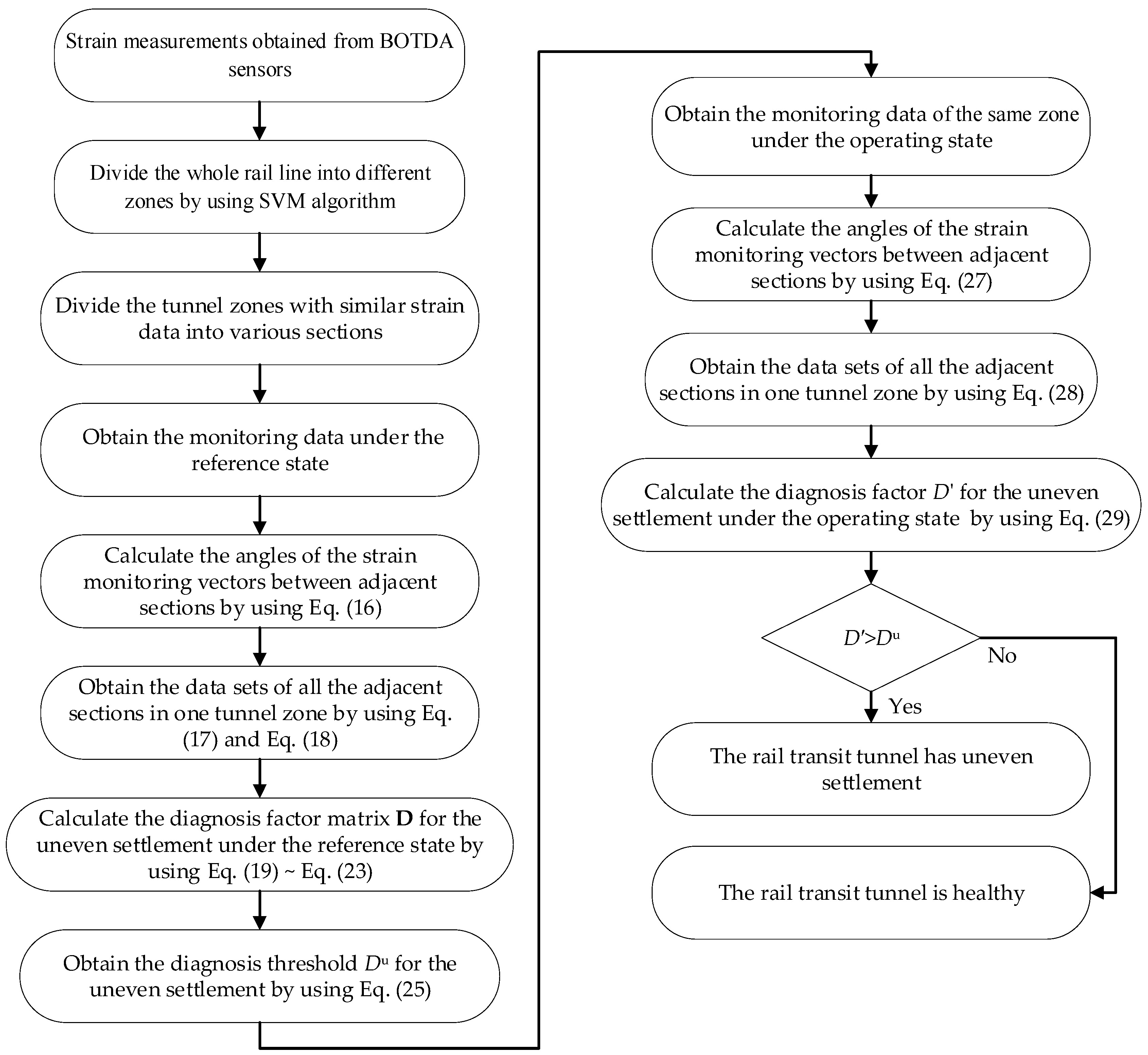
By comparing the diagnosis factors under the operating state with the corresponding diagnosis threshold, if any diagnosis factor under the operating state exceeds the corresponding diagnostic threshold, the corresponding area is considered to have uneven settlement; otherwise, the rail transit tunnel is considered to be healthy. The procedures for diagnosing the uneven settlement of rail transit tunnels based on the spatial correlation of high-density strain measurement points are shown in
Figure 3.
5. Numerical Example
5.1. Brief Description of an Actual Rail Transit Tunnel
Taking rail transit tunnel Line 3 in Jinan, China, as the research example, a finite element model is first established. The tunnel structure is composed of reinforced concrete segments, with an outer diameter of 6.4 m and an inner diameter of 5.8 m. There are four grades of surrounding rock, including levels III to VI, and the finite element model is built with level VI surrounding rock.
5.2. Generation of a Tunnel Finite Element Model
ANSYS software is applied to implement the numerical simulation. To simplify the calculation, only gravity is considered, and the Drucker–Prager model is selected to simulate the constitutive relation of the surrounding rock. The segments and the surrounding rock are simulated by SHELL181 and SOLID185 elements, respectively.
Theoretical analysis and practical research show that tunnel excavation has a certain influence on the surrounding rocks, and generally, the influence range is less than five times the tunnel diameter. Accordingly, the width and height of the surrounding rock in the model should be at least five times the tunnel diameter to eliminate the influence of the model boundary. Therefore, the model width, the distance from the lower part of the tunnel structure to the model bottom boundary and the model upper boundary are chosen to be 32 m, 20 m and 19.2 m, respectively. In addition, considering the computational cost, the length of the tunnel model is chosen to be 100 m.
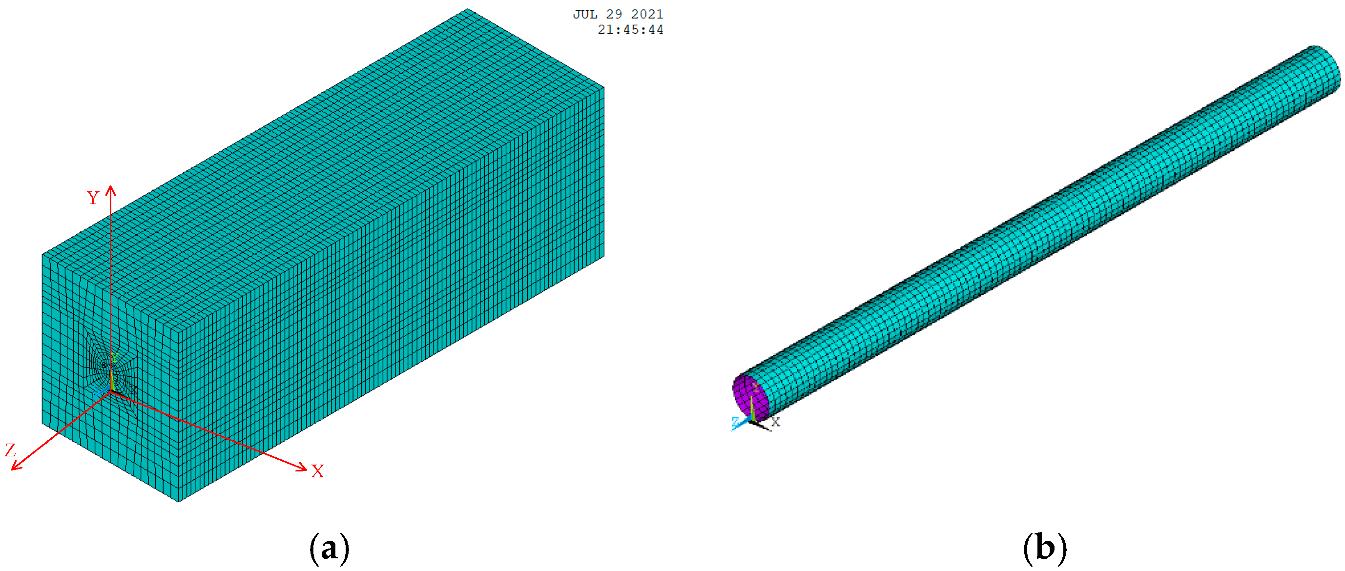
The boundary conditions imposed on the model are defined as follows. Considering this tunnel is a shallow-buried structure and the distance from the upper of tunnel to the road surface is less than 7 m, the upper boundary of tunnel is set free. The coordinate system of the finite element model is shown in
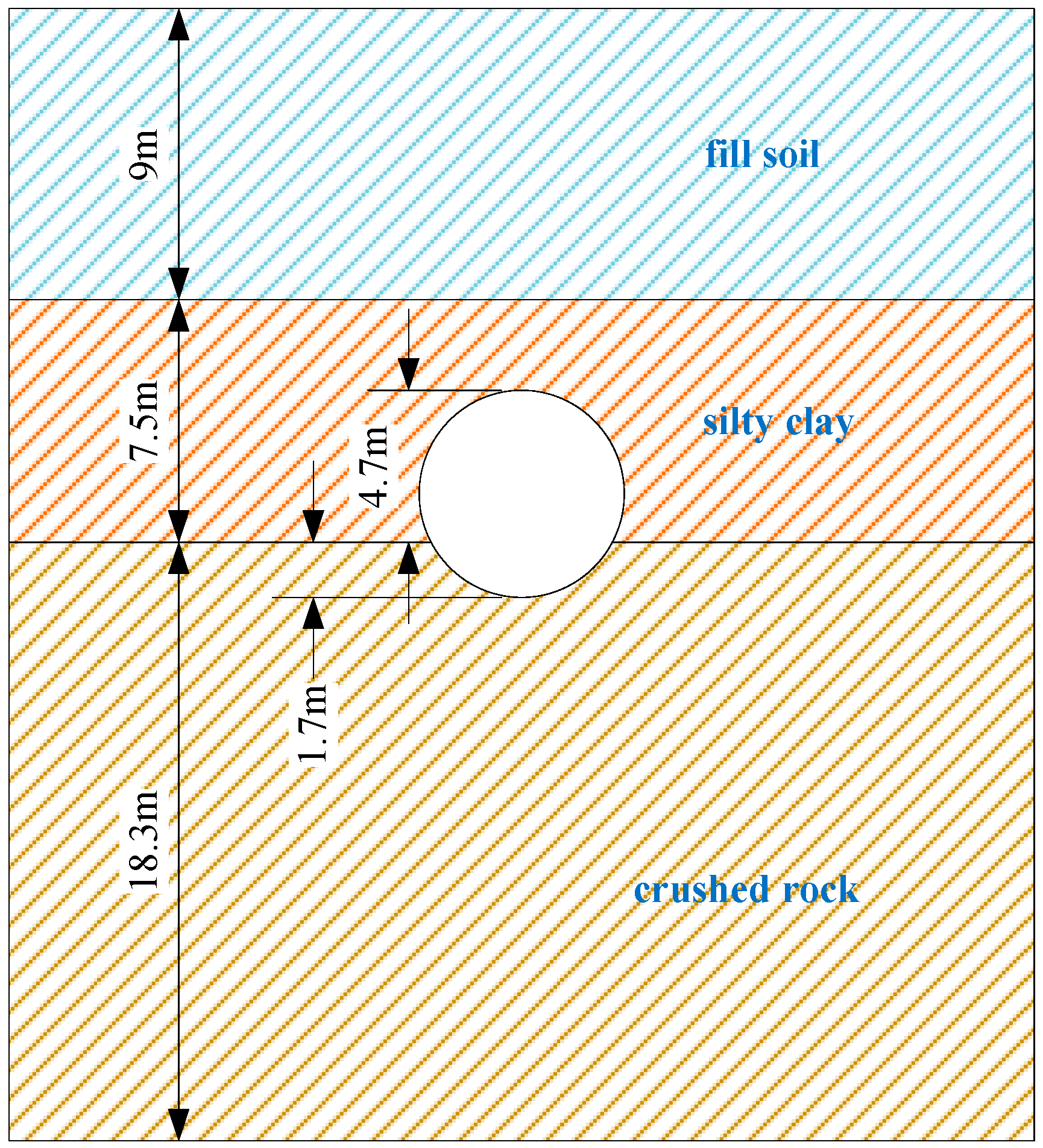
Figure 4. The left and right boundaries are only restricted along the X direction, and the lower boundary is only restricted along the Y direction. The front and back boundaries of tunnel are only restricted in the Z direction. The structural material of the tunnel is C50 concrete, and the surface soil includes three layers: fill soil, silty clay and crushed rock, from top to bottom, as shown in
Figure 5. The mechanical parameters of the main soil layers are listed in
Table 1.
The finite element model of the rail transit tunnel has a length of 100 m and a longitudinal grid size of 1 m, as shown in
Figure 4.
In the simulation of the uneven settlement of the rail transit tunnel, a 4 m-long segment is chosen, and the relevant nodes of the local tunnel shell element are displaced. Three degrees of local uneven settlement occurring at the middle of the tunnel model are simulated: a mild degree, a medium degree and a severe degree.
Since the longitudinal grid size of the finite element model is 1 m, we obtain data of 101 cross sections in total, of which the strain monitoring data at the bottom of the tunnel are used for diagnosis. In addition, 5 measuring points at both ends of the tunnel are excluded because of the boundary constraint effect, and 91 effective measuring points remain.
5.3. Verification of the Effectiveness of the Proposed Method
Using the calculated strain results under different conditions, further data processing is applied to simulate the variation in the data at different times, as in actual measurements, and 1000 sets of strain monitoring data are generated. For a single category, it is necessary to determine the lengths of the tunnel structure sections, which are related to the influence range of different uneven settlement degrees. In addition to the three abovementioned local settlement conditions, two more uneven settlement degrees are considered, including a minor degree and slightly severe degree, and the statistical influence ranges of the different uneven settlement degrees are shown in
Table 2.
According to the statistical results in
Table 2, it is obvious that the influence range is not very sensitive to the uneven settlement degree; therefore, we take 15 m as the generalized influence range under uneven settlement. In this case, the tunnel model is divided into six sections, and five vector angles of strain monitoring data between adjacent sections at each time point can be calculated, as shown in
Figure 6.
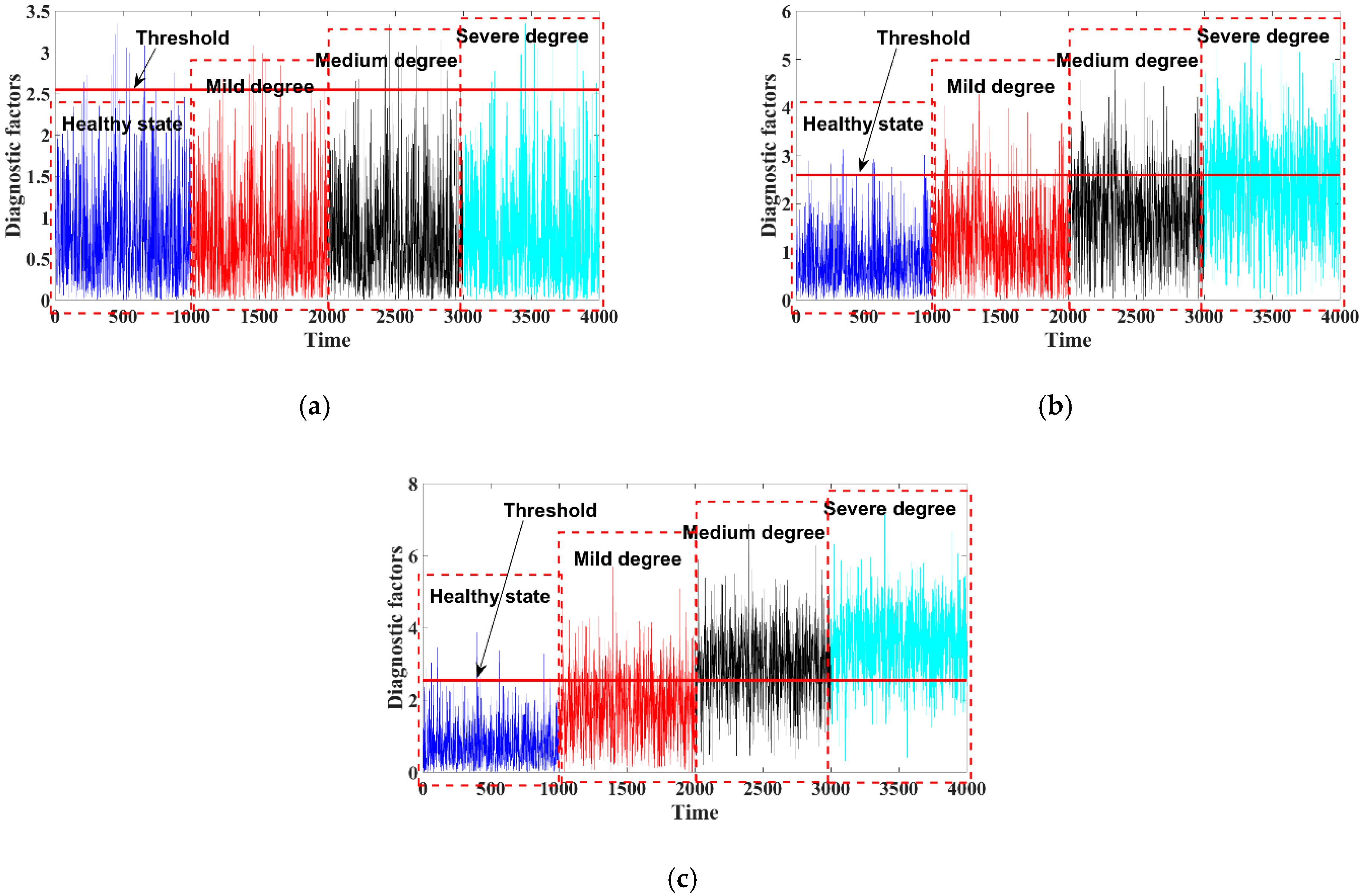
With the obtained data, five sets of diagnosis results for the adjacent sections can be calculated. Due to the structural symmetry, we need to diagnose the uneven settlement of adjacent tunnel sections 1–2, 2–3 and 3–4 only, and the diagnosis results are shown in
Figure 7. This figure shows that (1) the diagnosis effect becomes better with an increasing settlement degree; (2) for the adjacent sections 3–4, a mild degree of settlement can also be diagnosed effectively; and (3) for the adjacent sections 1–2, with a severe degree of settlement occurring in the middle of the tunnel, the diagnosis result appears to be healthy, which denotes diagnosis failure. Numerical results show that the proposed algorithm can diagnose uneven tunnel settlement effectively for the middle sections, while adjacent sections 1–2 may be influenced by the boundary constraint, causing this approach to fail to diagnose the uneven settlement there.
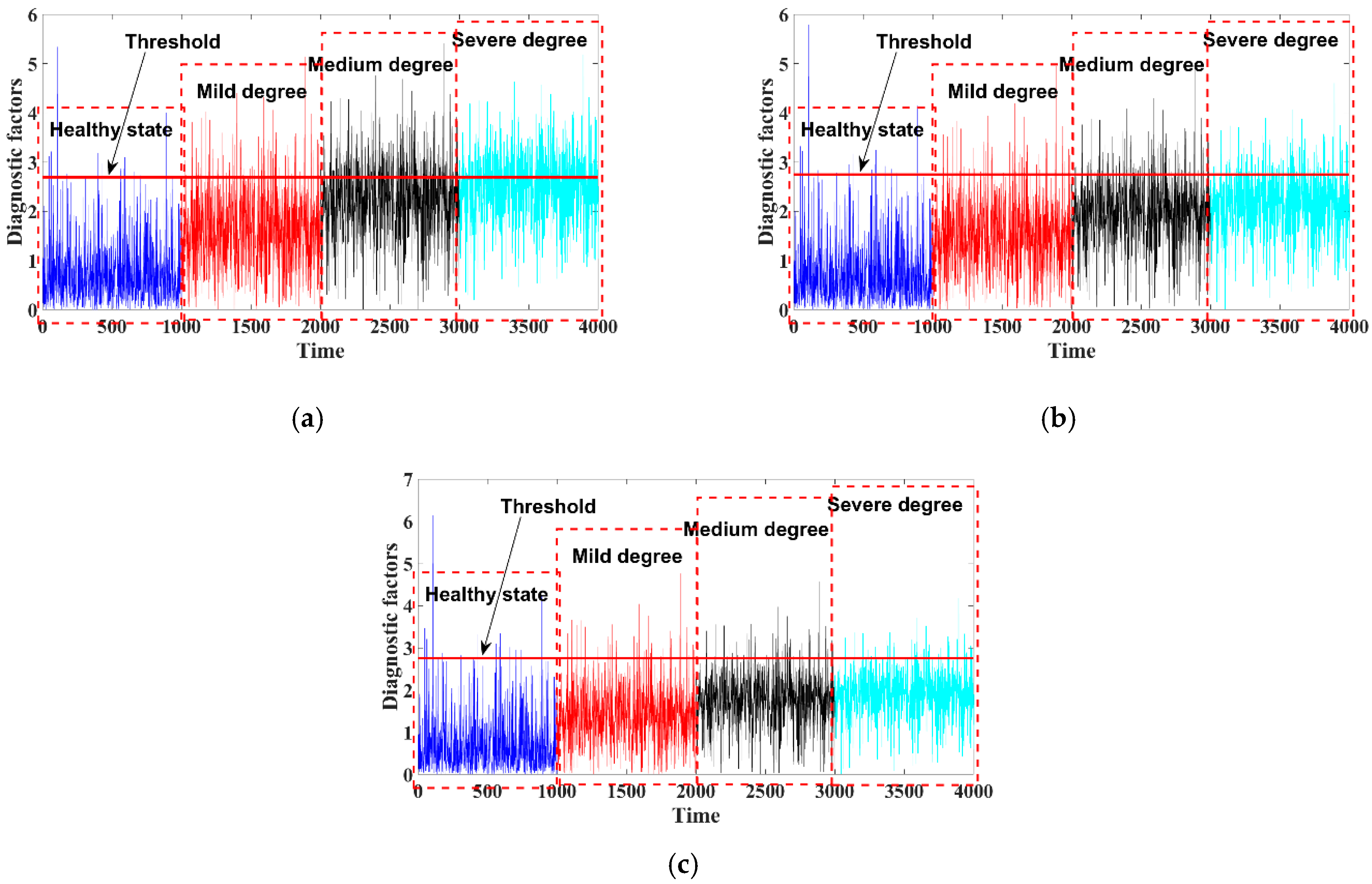
Considering the influence of noise on the diagnosis results, different levels of white Gaussian noise (5%, 10% and 15%) are introduced into the simulated strain data. Afterward, the noise-polluted data are used to calculate the diagnosis threshold under the reference state and the diagnosis factors under the operating state, and the diagnosis results of sections 3–4 are shown in
Figure 8.
As seen from
Figure 8, a mild degree of uneven settlement of the tunnel structure can be diagnosed even at the 10% noise level; however, it becomes difficult to diagnose when the noise level reaches 15%. The influence of the noise on diagnosing the uneven settlement of the tunnel is quantitatively studied by repeatedly applying noise. The test is repeated 100 times, and the results are as follows: the success rate for diagnosing a mild degree of uneven settlement of the tunnel structure under 5% noise level is 100%; the success rate for diagnosing a mild degree of uneven settlement of the tunnel structure under 10% noise level is 93%; the success rate for diagnosing a mild degree of uneven settlement of the tunnel structure under 15% noise level is 4%. The results show that the proposed algorithm is quite robust to noise.
6. Example of an Actual Rail Transit Tunnel
6.1. Arrangement of the Optical Sensing Fiber
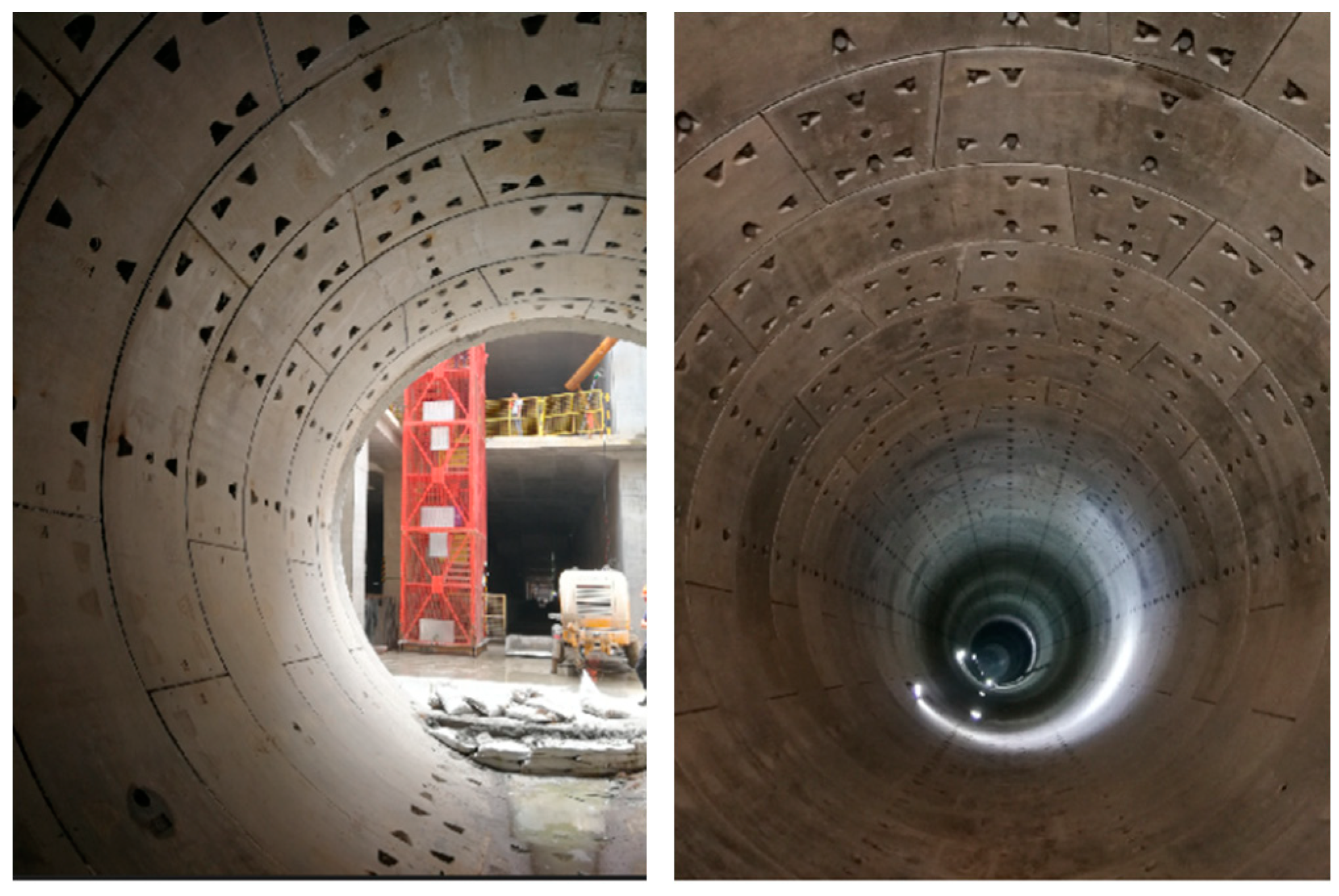
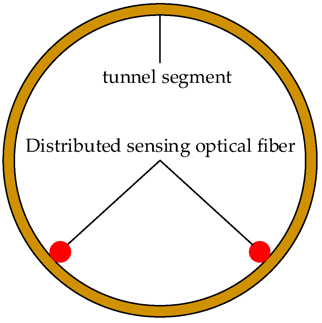
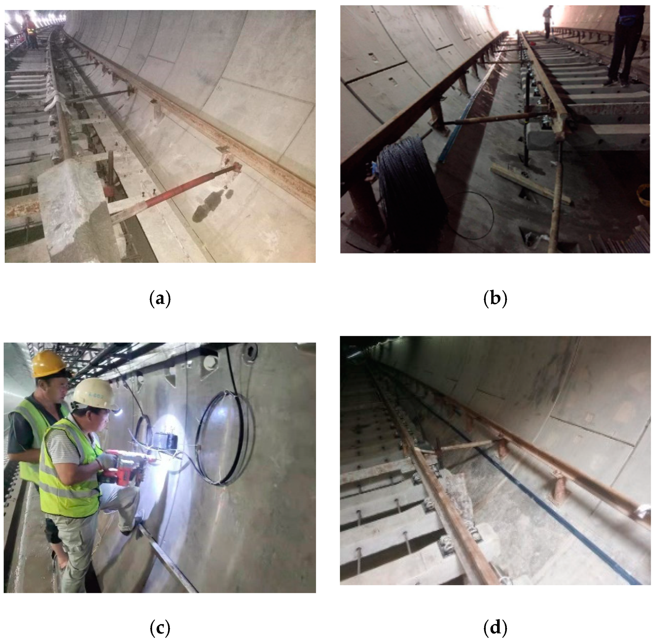
In the actual structure of rail transit tunnel Line 3 in Jinan, China, distributed Brillouin optical fibers are installed in the left tunnel along the tunnel line in a symmetrical form, and site photographs of the tunnel are shown in
Figure 9. The fibers were embedded 5~10 cm below the concrete surface, as shown in
Figure 10. Photographs of the optical fiber placement are shown in
Figure 11.
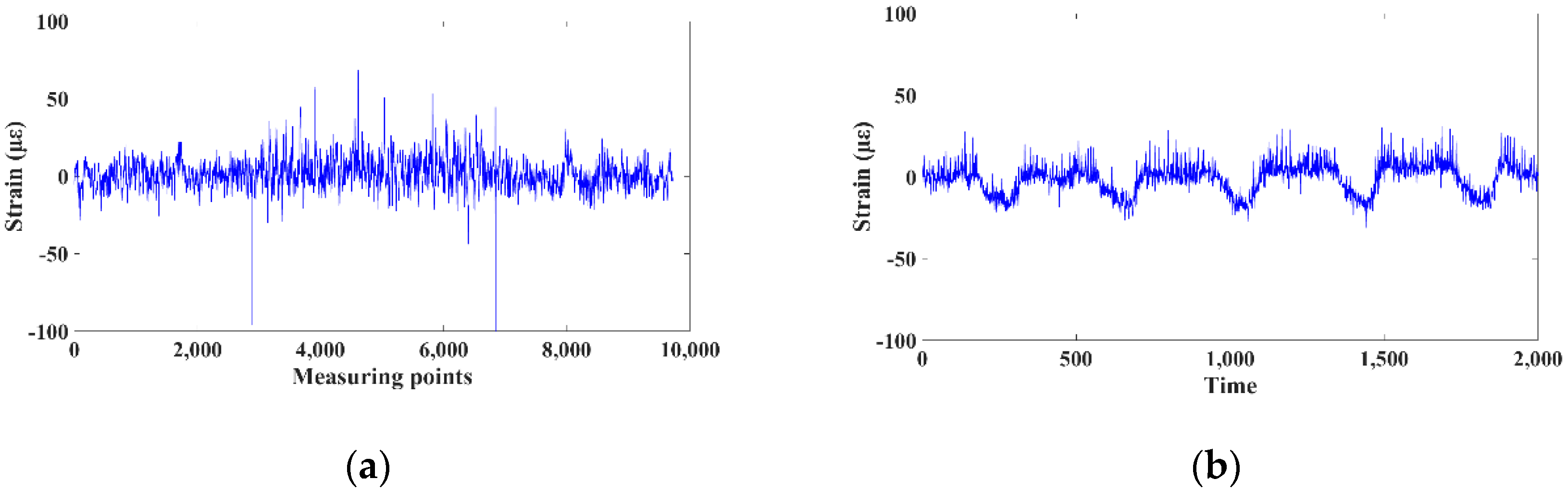
In the field test, 1 hour of monitoring data of the selected tunnel structural zones are collected, with a sample frequency of 1 min, and 61 sets of data are obtained in total. The length of the Brillouin optical fiber in this area is approximately 3965 m long, while the spatial resolution of the strain measurement points is 0.2 m, with 19,827 measuring points in total. The strain monitoring data of measuring points on the left side of the tunnel section at a certain time is shown in
Figure 12a, and the strain versus time of the middle measuring point in the tunnel structure is shown in
Figure 12b.
As shown in
Figure 12, most of the strain values are between −10 and 10 με, but there are still some anomalous data points with strains greater than 100 με, which may be caused by extrusion and sudden impact during the construction process; these data need to be excluded before the diagnosis of uneven settlement.
6.2. Cluster Analysis of Measured Data Obtained from BOTDA Sensors
Since the optical fiber is arranged symmetrically on the tunnel structure, monitoring data from only one side of the optical fiber are used here to diagnose uneven settlement. In the process of strain measuring point classification using the SVM algorithm, considering that the properties of the surrounding rock generally remain consistent in a wide range, almost 40 measuring points are selected to determine the optimal classification hyperplane.
According to the geological survey reports, there are four grades of surrounding rock, from level I to level IV. Using the monitoring data of selected measuring points, we obtain the optimal classification hyperplane to classify all the measuring points. Due to the continuity of structural and material properties, adjacent points can be grouped into the same category, and the final classification results are shown in
Figure 13. To study the robustness of the method for strain measuring point classification using the SVM algorithm, the values account for (VAF) were determined as per following basic mathematical expressions:
where
y and
y′ are measured and predicted values, respectively. In this study,
y′ is the final classification results as shown in
Figure 13, and the measured values of
y are obtained through geological survey. The calculation result of VAF is 82.5, and it shows that the method for strain measuring point classification using the SVM algorithm is effective.
Clearly, the measuring points can be roughly divided into four clusters, and there is a small region containing other types of measuring points between level I and level II; thus, this region is not taken into account to simplify the calculation. In other words, only the main four clusters of measuring points are used to diagnose uneven settlement.
6.3. Diagnostic Results of the Uneven Settlement of the Tunnel
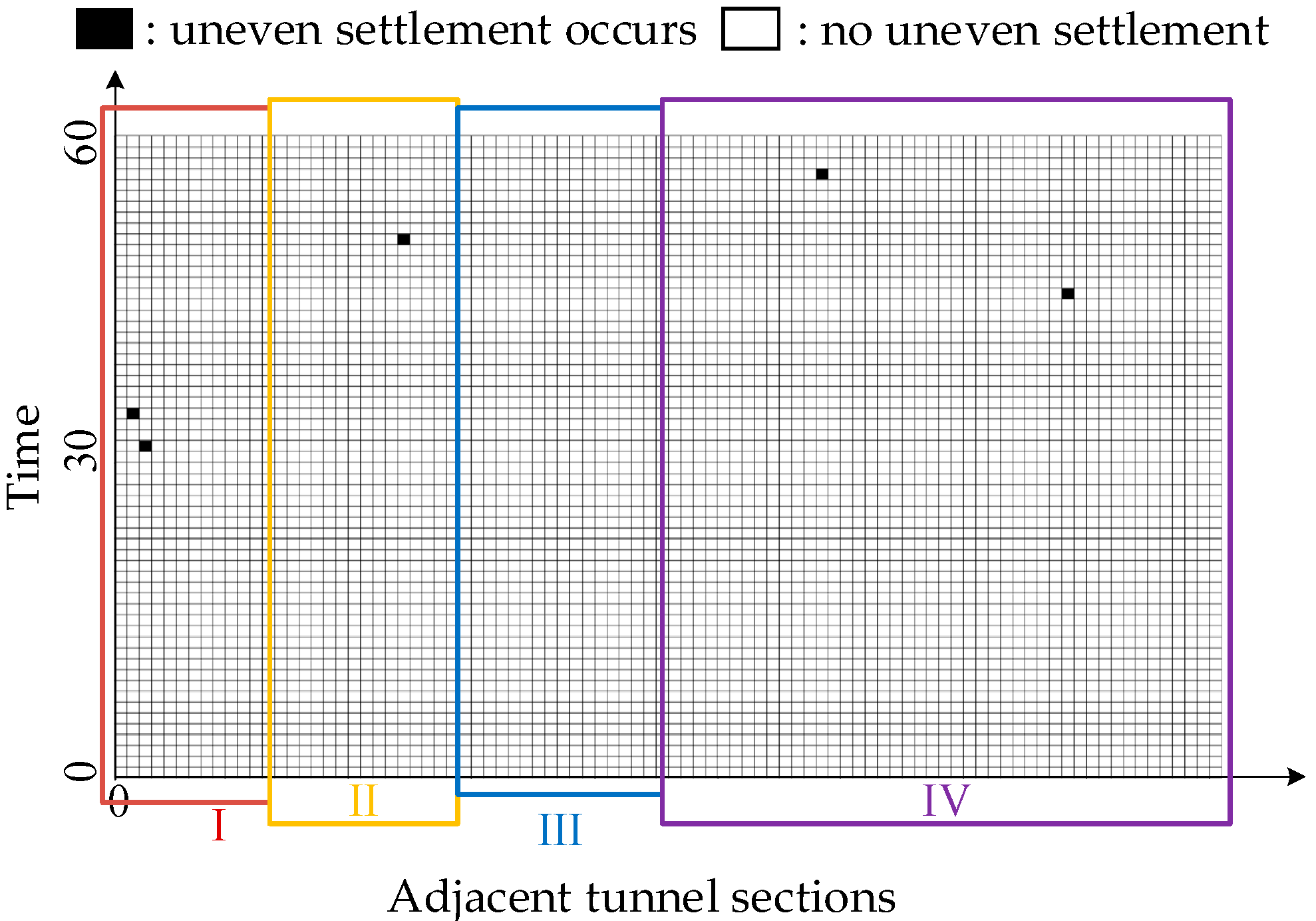
Based on the spatial correlation of the high-density strain measurement points, the monitoring data from the four classified measuring point clusters are used to diagnose uneven settlement. In this section, 20 m is taken as the division length of a tunnel section for the same tunnel category. On this basis, clusters I, II, III and IV are divided into 14, 16, 17 and 48 sections, respectively. The first 30 sets of collected data are taken as a healthy data set under the reference state to determine the diagnostic threshold, while the last 30 sets of data are regarded as the diagnosed data set under the operating state with which the diagnosis factors of uneven settlement are calculated.
To visualize the final diagnosis results, two states are considered: when the diagnosis factor exceeds the threshold, the mesh space is black, representing the occurrence of uneven settlement; otherwise, the mesh space appears to be white, representing the healthy state of the corresponding position. The results of all the positions and times form a grid diagram, as shown in
Figure 14.
As
Figure 14 shows, the diagnosis factors exceed the threshold in only a few instances, which may be induced by accidental sensor error, and further damage identification should be realized through long-term monitoring. Therefore, it can be judged that the tunnel was operating in a healthy state and that no uneven settlement had occurred, verifying the effectiveness of the proposed method.
As discussed above, with the distributed optical fiber sensing technique, the proposed method can diagnose whether uneven settlement of the tunnel structure has occurred. Owing to the high-density strain measurement points, it is effective for the proposed method to localize the uneven settlement of tunnel. However, it is difficult for the proposed method to accurately quantify the magnitude of uneven settlement of tunnel. Therefore, for the further research, we mainly focus on how to determine the accurate magnitude of settlement deformation occurred on tunnel.


