Evolution of the Spatial Pattern of the Assets and Environmental Liabilities Conversion Rate and Its Influencing Factors

Abstract

With the extensive development of the economy, environmental degradation has become a serious global issue. How to ensure the sustainable development of regional environments has drawn widespread attention from governments, academia, and the public. As an index to measure the efficiency of financial expenditure on the environment by local governments, the assets and environmental liabilities conversion rate (AELCR), along with the spatial pattern changes it presents and the factors it is affected by, is worthy of in-depth study. This study took the AELCRs of 31 provinces in China from 2012 to 2017 as the research objects, analyzed their spatial patterns and evolution using GeoDa software, and explored their spatial distribution using a spatial econometric model. The results show that, on the whole, China’s provinces were characterized by unbalanced economic development and large gaps in development levels, and there were significant differences in the efficiencies of fiscal expenditure for environmental protection between regions. Overall, there was a negative correlation between China’s neighboring provinces, and there was strong heterogeneity between provinces with a low conversion efficiency and the surrounding provinces. Locally, most provinces did not show significant spatial correlation, while the local similarities of the AELCRs decreased from 2012 to 2017, and the heterogeneities increased. Through the analysis of influencing factors, it was found that the urbanization level and provincial R&D investment positively increased the AELCRs, where the positive impact of urbanization was more obvious; resource tax and urban infrastructure investment were negatively correlated with the conversion rates, and the negative impact of resource tax was greater. The findings of this study provide important theoretical and practical implications for local governments to reasonably allocate environmental expenditure and improve their conversion rate of assets and environmental liabilities.

1. Introduction

With the Industrial Revolution of the 18th century, steam machines using coal as energy were widely used, and the global economy developed rapidly. However, industrial pollution not only destroyed the ecological environment but also threatened people’s health. Since its reform and opening up, China’s economy has been developing rapidly for 30 years due to the large consumption of resources; however, the extensive economic growth mode makes the environmental burden more serious. With the rapid consumption of natural resources, environmental problems emerged one after another. According to the statistics of China’s Environmental Protection Bureau, the proportion of China’s total investment in pollution control relative to GDP is increasing year by year, but environmental pollution emergencies are also increasing year by year. The negative externalities of resource consumption and environmental problems require governments to continuously explore feasible solutions, such as environmental protection taxes and carbon emissions trading. The Environmental Protection Act was formally implemented in China on 1 January 2015. The opinions of the State Council regarding strengthening the key work of environmental protection (GF (2011), No. 35) were promulgated in November 2011, requiring that “environmental protection should be included in the annual budget at all levels, and investment should be gradually increased, and funding arrangements for environmental protection capacity building at the same level should be increased at the right time.”

Currently, data envelopment analysis (DEA) and its extended model are widely used for evaluating the efficiency of local government assets and environmental conversion. Few studies have comprehensively measured and evaluated the efficient conversion of assets and environmental liabilities in China from the geospatial perspective. At the same time, there have been few systematic studies on the spatial evolution characteristics and influencing factors of resources and environmental efficiency at national and urban scales. Studying environmental assets from the spatial perspective, exploring the regional impact on the evaluation of environmental asset conversion efficiency, and studying the interactions between different regions in China can enrich the methods and ideas of environmental asset evaluation.

Based on this and other scholars’ research, this study adopted a way of thinking about accounting that breaks from the traditional limitation of using the efficiency of converting from economic assets to environmental liabilities to evaluate the performance of local environmental governance. Taking 31 provinces of China as decision-making units, this study used a Super-SBM model to measure the conversion efficiency between local government assets and environmental liabilities. At the same time, a spatial weight matrix was established, and spatial correlation analysis and a spatial econometric model were used to analyze and explore the law and dynamic change trends in provincial government conversion efficiency from the perspective of main functional areas. It was concluded that the SLM model, which is different from the existing Malmquist index, was more suitable for analyzing dynamic changes in conversion efficiency, enriching the existing research results.

2. Literature Review

2.1. Research on Environmental Liabilities

Environmental liability refers to the responsibility of humans to restore and improve the ecological environment and make sustainable use of natural resources in the future. It is a “realistic obligation” to restore the environment. This is also the kind of obligation that people should take on in the process of developing and utilizing resource assets, which can be measured using currency, and that needs to use other assets or services to repay. At the same time, it is also the economic essence of environmental liabilities [1]. The assets that are closely related to environmental liabilities can be divided into two categories: economic and resource assets. Economic assets refer to the amount of financial expenditure that is invested by local governments to perform their environmental protection functions and the infrastructure and equipment for environmental protection and pollution control that are formed on this basis [2]. China’s resource assets mainly include energy, minerals, land, forest, and water [3].

Currently, research on environmental liabilities is focused on evaluating the efficiency of environmental protection expenditure. Previous studies found that the efficiency of such expenditure in most regions of China is at a low level, the financial investment in environmental governance shows a diminishing scale effect, and the investment cannot effectively improve environmental quality. China’s fiscal budget expenditure does not show a scale effect, external effect, or environmental effect but only a transfer payment effect. As the leader of regional ecological civilization construction, the government plays an important role in environmental protection. However, by blindly increasing investments in economic assets for environmental protection, it is difficult for local governments to meet these needs, and the effect of environmental governance shows a trend of marginally decreasing. Therefore, local governments should invest in the environment in a planned and reasonable way to improve the utilization efficiency of funds and avoid the situation of acquiring half the results with twice the effort.

2.2. Efficiency Calculation and Index Selection for Environmental Protection Expenditure of Local Government

Among various research methods available within the empirical literature, data envelopment analysis (DEA) and its extended model are the main way to evaluate and analyze the efficiency of local environmental governance [4]. DEA was first proposed by Charnes, a famous operational research expert, in 1978 and is a common method for measuring production efficiency. It was first introduced in terms of evaluating environmental efficiency by Färe et al., who used inputs and outputs to measure pollution variables [5]. Chung et al. developed a new DEA model combined with the direction distance function. In the performance analysis, the direction vector should be set first to improve the decision unit performance along the direction, and then the desirable outputs can be increased and the pollution decreased; such a method further expanded the research on the efficiency of environmental protection expenditure [6].

In the early research, the amounts of investment in infrastructure, industrial pollution source treatment, and environmental protection were usually used as input variables to measure the efficiency of environmental treatment, while the actual removal amounts of smoke, dust, and sulfur dioxide and the total output value of the comprehensive utilization of these three waste products were used as output variables to measure the efficiency of environmental governance [7,8,9]. With the deepening of research and increasing awareness of environmental protection, natural resource assets are gradually incorporated into the evaluation system of environmental governance efficiency; for example, water, forest, land, and other resource assets are used as input indicators [10]. The results of environmental governance efficiency assessment not only can help each region to carry out self-examination but also can help in carrying out horizontal comparisons, understanding the utilization efficiency of environmental resources between regions, and providing an effective reference for improving environmental governance [11,12,13].

2.3. Factors Influencing the Conversion Rate of Assets and Environmental Liabilities

In research on the factors affecting the conversion rate of assets and environmental liabilities, most scholars at home and abroad focus on economic development, institutional factors, etc. One study found that city size and fiscal revenue have an important impact on the efficiency of regional fiscal expenditure [14]. Based on the interaction mechanism between urbanization development and the urban ecological environment, Li et al. proposed an evaluation system that is based on urbanization development, with the belief that urbanization processes based on population development, industrial institutions, and social activities will affect the efficiency of regional environmental governance [15]. Liu et al. found that, in addition to the urbanization level, the regional economic development level and FDI will also affect the efficiency of regional environmental governance [16].

In addition to the traditional economic, institutional, and regional factors, new perspectives, such as energy consumption and public participation, have gradually become factors that influence the assets and environment liability conversion rate. Policy orientation, government attention, environmental awareness, and other factors have a significant impact on the conversion rate of regional assets and environmental liabilities [17]. At the same time, government corruption reduces the efficiency of local environmental governance [18]. The level of government management is an invisible factor that enhances environmental governance efficiency [19]. The loss of natural resources is considered to be the biggest obstacle to improving environmental efficiency [20]. Spatial heterogeneity also affects environmental governance efficiency [21,22].

To summarize, research on the conversion of environmental assets and liabilities is still in the development stage, and the DEA and its extended model are mostly used for evaluating the conversation rate for local governments. The current research evaluating the efficiency of local environmental governance is still focused on economic performance, is less frequently used for environmental benefits, and rarely analyzes the spatial evolution characteristics and influencing factors of the conversion rate of environmental assets and liabilities from the geospatial perspective. Based on this, we selected the conversion rate of assets and environmental liabilities as the index and used the convertibility of resource assets to calculate the conversion rate in each region using the Super-SBM model, with undesirable outputs proposed by Tone [23], taking each region of China as a decision-making unit. Afforested areas, underground water supply, and the reduction of environmental pollution were included in the research framework, breaking the traditional limitation of using a single economic indicator to evaluate the performance of environmental governance and enriching and improving the selection of input and output indicators. At the same time, the use of spatial correlation and spatial econometric model analyses helped to determine the dynamic change rules, trends, and influencing factors of the assets and environmental liabilities conversion rate in various regions, which expanded the research ideas regarding the conversion rate, helped to analyze the source variables, and guided the evaluation of the efficiency of environmental protection financial expenditure activities.

2.4. Research Hypotheses

By evaluating the related existing research theories and associated literature, we found that the main influencing factors of environmental efficiency in our provinces were economic scale, industrial structure, degree of opening to the outside world, government regulation, technological progress, and regional characteristics. The assets and environmental liabilities conversion rate represents the efficiency of regional environmental governance, and the level of regional economic development affects the local government revenue. On the one hand, the higher the level of economic development, the more the local government can invest in environmental protection. On the other hand, a high level of economic development often means an improved per capita income, which will stimulate people’s demand for a high-quality environment and help to improve environmental efficiency [24,25]; therefore, when per capita GDP increases, it will help to improve the assets and environmental liabilities conversion rate.

Infrastructure is significant for the national and regional socioeconomic activities of the public service system, which encompasses more than simply economic interests, and is very important for social development [26]. The urban environmental infrastructure is closely related to the protection and improvement of the urban environmental quality, including garbage and sewage treatment facilities, city appearance, and sanitation facilities. Garbage and sewage treatment facilities can reduce pollution and improve environmental quality by centralizing the collection and treatment of garbage and wastewater [27]; thus, the operational efficiency of environmental infrastructure directly affects the quality of the urban environment.

Some studies also found that improving environmental efficiency mainly depends on the overall progress of green technology in the region [28] and that innovation is conducive to green growth efficiency [29]. On the one hand, technological innovation can improve the reuse of pollution emissions, that is, the end treatment of environmental pollutants. On the other hand, technological innovation can improve the efficiency of resource use and reduce the amount of pollution emissions by forming a front-end defense through advanced technology [30].

The level of urbanization also has an impact on the assets and environmental liabilities conversion rate. With the active promotion of urbanization by the Chinese government, the urban population density is gradually increasing. The increased population density will require adaptive changes in the industrial structure and spatial layout of urban functions, which may have negative effects on the environment, such as the greenhouse effect and deteriorated water quality [31,32]. However, it was also suggested that the process of urbanization will improve labor productivity, change the economic structure, and alleviate the growth trend of industrial pollution emissions [33,34]; at the same time, with the increased urbanization rate, the population density will increase. The positive effects of improving living standards, education levels, and environmental awareness that are brought by the increased population density on environmental efficiency are greater than the negative effect of increased pressure on the ecological environment. The levels of urbanization and economic development are conducive to improving the efficiency of local environmental governance expenditure [16].

Due to the negative social externalities, resource taxes have gradually become an important means to control environmental pollution. However, energy taxes can also increase economic costs, weaken the international competitiveness of enterprises and industries, reduce economic output, and damage economic growth [35]. Based on the perspective that environmental quality and leisure time affect residents’ welfare, Schwartz and Repetto [36] considered the idea that employment is not only affected by the macro-economy but is also closely related to changes in the quality of the environment and health. Therefore, by levying environmental taxes, the “double dividend” of environmental protection and economic growth can be obtained. However, Pautrel [37] found that, based on the perspective of general equilibrium, the tax distortion effect will become more serious, and increased resource taxes will lead to increased redundancy of environmental governance investment. Based on the aforementioned, we proposed the following hypotheses:

Hypothesis 1 (H1a).

There is a positive relationship between the level of regional economic development and assets and environmental liabilities conversion rate.

Hypothesis 1 (H1b).

There is a positive relationship between the urban environmental infrastructure and assets and environmental liabilities conversion rate.

Hypothesis 1 (H1c).

There is a positive relationship between technological innovation and the environmental liabilities conversion rate.

Hypothesis 1 (H1d).

There is a positive relationship between the level of urbanization and the environmental liabilities conversion rate.

Hypothesis 1 (H1e).

There is a negative relationship between resource taxes and the environmental liabilities conversion rate.

3. Methodology

3.1. Transformation Logic and Model Selection of Assets and Environmental Liabilities

Marlin [38] proposed the idea that environmental accounting is actually the measurement of the conversion relationship between man-made and natural resources. Resource assets are essential elements for improving the quality of the environment, which have their own characteristics regarding quantity, time, quality, and so on [39,40], and cannot be replaced by man-made assets. In the long run, resource assets play an important role in repairing and improving regional environmental quality problems and reducing environmental liabilities, and the ecological and economic value can be transformed [41]. Environmental liability is present due to development activities in the past and refers to the amount of environmental remediation that currently needs to be carried out, which is a strong externality [42]. Local governments achieve the goal of public service by investing in environmental protection, that is, by controlling environmental pollution and preventing environmental degradation. The investment in environmental protection and various environmental control facilities and equipment constitutes the economic assets used by local governments to protect the environment [43].

Against the background of fiscal decentralization of the Chinese government, the amount of special funds for environmental protection that is allocated by the central government budget is limited, and local governments bear greater responsibility for the expenditure and disbursement of such funds. In order to further improve the environmental quality for residents in various regions, the government needs to increase the proportion of special funds for environmental protection in the total budget, which is mainly reflected in increased government resource assets or decreased environmental liabilities. For example, Hainan Province has better natural resource endowment, rich resource assets, and fewer environmental liabilities to be borne by the government. Therefore, the government’s expenditure on environmental protection mainly increases economic or man-made resource assets that are used for environmental protection. In contrast, although the types of resource assets are relatively scarce in Shanghai, the government has environmental liabilities. The environmental protection expenditure by the Shanghai municipal government mainly increases the economic assets that are used for environmental restoration. Based on the above analysis and methods of accounting, this study deduced the following identities of the dynamic accounting equation [44]:

Economic Assets = Resource Assets − Environmental Liabilities

Of course, in the process of local environmental governance, some local governments will blindly pursue GDP growth at the expense of the environment and natural resources, forming a “vicious cycle” of competition, which is not conducive to regional sustainable development. Eventually, the increment of economic assets invested by local governments will be negative, which is mainly reflected in the quantity of man-made resource assets and natural resources. The responsibility for decreases in source assets or increases in environmental liabilities should be borne by local governments. In short, when the amount of economic assets invested by local governments is zero, the decreased investment will inevitably lead to increased environmental liabilities that local governments should bear. According to the nature of government environmental accounting subjects, there is an “allowance relationship” between local government resource assets and economic assets.

3.2. Efficiency Evaluation Using the Super-SBM Model with Undesirable Outputs

Tone constructed a new DEA model called the slack-based measure (SBM) DEA [23]. The slack variables in the SBM model are directly added into the target function; the SBM method is thus non-radial and manages input/output slacks directly, and it avoids radial and oriented deviation, which is better than any other model for solving the defects of the traditional DEA model and reflecting the nature of the efficiency evaluation. In addition, modern production and life are often accompanied by undesirable outputs; therefore, Tone proposed the Super-SBM model to measure efficiency in the presence of undesirable outputs. The Super-SBM model can more truly reflect the nature of the evaluation of the conversion efficiency of the local government’s resource assets, economic assets, and environmental liabilities.

According to the model proposed by Tone, we considered a production system with n DMUs. Each unit had three factors: input, desirable outputs, and undesirable outputs, represented by three vectors: $x\in R^m$, $y^g\in R^{s_1}$, and $y^b\in R^{s_2}$. We defined the matrices $x$, $y^g$, and $y^b$ as follows:

$$P=\left\{\left(x,y^g,y^b\right)|x\ge X\lambda ,y^g\le Y^g\lambda ,y^b\ge Y^b\lambda ,\lambda \ge 0\right\}$$

(1)

In Equation (1), λ is the weight vector. When ${\displaystyle \sum {\lambda }_i}=1$, the limit is added, and the SBM model with variable scale compensation is obtained:

$$\rho =\mathrm{Min}\frac{1-\frac{1}{m}{\displaystyle \sum _{i=1}^m\frac{S_{{}_i}^{-}}{x_i{}_{{}_0}}}}{1+\frac{1}{s}{\displaystyle \sum _{r=1}^m\frac{S_{{}_i}^{+}}{y_r{}_{{}_0}}}}$$

(2)

$$s.t.\{\begin{array}{c}{x}_0=X\lambda +S^{-};\\ y_0^g=Y^g\lambda -s^g;\\ y_0^b=Y^b\lambda +s^b\\ s^{-}\ge 0,s^g\ge 0,s^b\ge 0,\lambda \ge 0\end{array}$$

(3)

When $\rho$ is equal to 1, DMU is effective; when ρ is less than 1, DMU is invalid, and the indicators in the model need to be adjusted. Compared with the traditional DEA model, SBM has many advantages, but it cannot measure efficiency in the case of an undesirable output. If we do not distinguish the desirable outputs from the undesirable outputs, thereby mixing the two, this will be contrary to the constraints set by the model and will affect the results.

$$P|\left(x_0,y_0\right)=\left\{\left(x,{\overline{y}}^g,{\overline{y}}^b\right)|\overline{x}\ge {\displaystyle \sum _{j=1}^n{\lambda }_j}{x}_j,{\overline{y}}^g\le {\displaystyle \sum _{j=1}^n{\lambda }_j}{y}_j{}^g,{\overline{y}}^b\ge {\displaystyle \sum _{j=1}^n{\lambda }_j}{y}^b,{\overline{y}}^g\ge 0,\lambda \ge 0\right\}$$

(4)

However, in most situations in efficiency evaluation research, the best performers have a full efficiency status that is denoted by 100%; from experience, we know that multiple decision-making units usually have this ‘‘efficient” status. Therefore, it is meaningful in the analysis of efficiency rankings and influential factors to discriminate between these efficient DMUs. To provide more accurate values for the efficiency analysis, this study combined the study of Tone [23] based on the SBM model to give the Super-SBM model with undesirable outputs, which was used for evaluating the SBM-efficient DMUs. The model with undesirable output was as follows:

$$\rho *=\min \frac{\frac{1}{m}{\displaystyle \sum _{i=1}^m\frac{x_{{}_i}^{-}}{x_i{}_{{}_0}}}}{\frac{1}{s_1+s_2}\left({\displaystyle \sum _{r=1}^{s_1}\frac{{\overline{y}}_r^g}{y_{{}_r}^g{}_{{}_0}}}+{\displaystyle \sum _{t=1}^{s_2}\frac{{\overline{y}}_r^b}{y_{{}_r}^g{}_{{}_0}}}\right)}$$

(5)

$$\begin{array}{l}s.t.\overline{x}\ge {\displaystyle \sum _{j=1,\ne 0}^n{\lambda }_j}{x}_j,{\overline{y}}^g\le {\displaystyle \sum _{j=1,\ne 0}^n{\lambda }_j}{y}_j{}^g\\ {\overline{y}}^b\ge {\displaystyle \sum _{j=1,\ne 0}^n{\lambda }_j}{y}^b,\overline{x}\ge x_0,{\overline{y}}^g\le {\overline{y}}_0^g,{\overline{y}}^b\ge y_0^b\\ {\displaystyle \sum _{j=1,\ne 0}^n{\lambda }_j=1},{\overline{y}}^b\ge 0,\lambda \ge 0\end{array}$$

(6)

Equation (5) is the target efficiency value, which indicates the conversion efficiency of the environmental assets and liabilities of the local government. The other variables are the same as in Equation (2). Overall, the Super-SBM model with undesirable output has outstanding advantages: it takes undesirable outputs into account when evaluating economic efficiency and is different from the traditional DEA model. It can sort the efficiency of multiple DMUs and solve the problem of redundancy regarding input and output indicators.

3.3. Spatial Econometric Model and Estimation Method

The conversion rate of assets and environmental liabilities mainly examines the efficiency of local government environmental protection expenditure and regional natural resources, and based on the correlation or difference between different regions in China, this indicator may be affected by the surrounding regional environment. Spatial metrology is based on geographic data, which is used to analyze the development of spatial observations [45]. Spatial autocorrelation refers to the potential interdependence of some variables in the same distribution area. Spatial autocorrelation statistics are used to measure a basic property of geographic data: the degree of interdependence between data in different locations [46]. This is usually called spatial dependency. Due to the influence of spatial interaction and diffusion, geographic data may be correlated. Therefore, this process can be defined as “the calculation of spatial autocorrelation degree between a certain spatial unit and its surrounding units in a space through statistical method, so as to analyze the characteristics of spatial distribution phenomenon of these spatial units.” Therefore, we used the spatial autocorrelation analysis model to analyze the spatial evolution characteristics of the conversion rate of assets and environmental liabilities in each province, evaluated the environmental resources from the regional perspective, and used the model to determine the factors that affected the spatial evolution characteristics of the conversion rate, which is helpful for local governments to implement policies and improve the efficiency of regional governance.

3.3.1. Spatial Autocorrelation Analysis Model

(1) Global spatial autocorrelation

Global spatial autocorrelation is used to measure whether there is a correlation in the spatial distribution of a phenomenon in a whole research area. It reflects the spatial distribution of activities in the whole area [45]. Moran’s I is the most frequently used variable in spatial correlation analysis. The formula that is used to calculate Moran’s I is as follows:

$$Mora{n}^{\prime }sI=\frac{{\displaystyle \sum _{i=1}^n{\displaystyle \sum _{j=1}^m{W}_{ij}\left(Y_i-\overline{Y}\right)\left(Y_j-\overline{Y}\right)}}}{S^2{\displaystyle \sum _{i=1}^n{\displaystyle \sum _{j=1}^n{W}_{ij}}}}$$

(7)

where $S^2=\frac{1}{n}{\displaystyle \sum _{i=1}^n\left(Y_i-\overline{Y}\right)}$; $\overline{Y}=\frac{1}{n}{\displaystyle \sum _{i=1}^{n}Y}$, $Y_i$ is the observation value of the ith geographical unit, n is the number of geographical units, and $W_{ij}$ is the standard adjacency matrix.

The value range of Moran’s I is generally [−1,1]. A positive value means that there is a positive spatial correlation between the geographical observation units and similar attribute values, a negative value means that there is negative spatial correlation and dissimilarity between units, and a value of zero means the observed units are independent of each other.

The results of Moran’s I were tested using an approximate normal distribution and standardized.

$$Z(d)=\frac{Mora{n}^{\prime }sI-E(I)}{\sqrt{{\delta }^2(I)}}$$

(8)

$$Mora{n}^{\prime }sI{\delta }^2{}_n(I)=\frac{n^2{w}_1+n{w}_2+3w_0^2}{w_0^2\left(n^2-1\right)}-E_n^2(I)$$

(9)

$$\begin{array}{c}\hfill Mora{n}^{\prime }sI{E}_n(I)=-\frac{1}{n-1};\\ \hfill W_0={\displaystyle \sum _{i=1}^n{\displaystyle \sum _{j=1}^n{W}_{ij}}};W_1=\frac{1}{2}{{\displaystyle \sum _{i=1}^n{\displaystyle \sum _{j=1}^n\left(W_{ij}+W_{ji}\right)}}}^2;W_2={{\displaystyle \sum _{i=1}^n\left(W_i+W_j\right)}}^2\end{array}$$

(10)

where $W_i$ is the sum of I rows in the spatial weight matrix, and $W_j$ is the sum of J columns in the spatial weight matrix. When $\left|Z\right|>1.64$, Moran’s I is significant within a 99% confidence interval; when $\left|Z\right|>1.96$, it is significant within a 95% confidence interval.

(2) Local spatial autocorrelation

Local spatial autocorrelation is used to reflect the degree of correlation between features in adjacent units, which is the local indicator of spatial association (LISA) [47]. The LISA of each geographical observation unit indicates the degree of spatial agglomeration with similar units that pass a significance test:

$$Mora{n}^{\prime }s{I}_i=Z_i{\displaystyle {\sum }_{j=1}^n{W}_{ij}{Z}_j}$$

(11)

where $W_{ij}$ is the spatial weight matrix; therefore, Moran’s I can be expressed as a deviation of the observed value, where i and j are deviations of the values of the observed unit i and adjacent unit j. Moran’s I > 0 indicates that there are similar spatial clusters in the geographical observation units; Moran’s I < 0 indicates that there are different clusters.

3.3.2. Spatial Regression Model

A spatial regression model introduces spatial effects into fixed spatial coefficients. By combining attribute data with spatial positions, spatial regression can better explain the spatial relationships between geographical objects. We used spatial lag and spatial error models to explore the factors that affected the spatial evolution characteristics of the conversion rate.

(1) Spatial Lag Model (SLM)

The spatial lag model, also known as the spatial autoregressive model, mainly examines whether the spatial dependence of the variables of geographical observation units produces a spillover effect, which reflects the idea that the influencing factors of the dependent variables will affect other areas through spatial transmission mechanisms:

$$Y=\rho Wy+X\beta +\epsilon$$

(12)

where Y is the dependent variable, X is an independent variable matrix of order $n\times k$, W is the spatial weight matrix of $n\times n$, $W_{ij}$ is the spatial lag term of the dependent variable, and ε is the random error term.

(2) Spatial Error Model (SEM)

In the spatial error model, the degree of spatial autocorrelation of the error term can be used to express the influence of the dependent variable error in the adjacent area on the dependent variable error of the observed unit, which reflects the idea that regional spillover is the result of a random rush out. This indicates that the spatial disturbance term is related to the spatial population, and spatial disturbance in one space will affect other spaces:

$$\begin{array}{l}Y=X\beta +\epsilon \\ \epsilon =\lambda W\epsilon +\mu \end{array}$$

(13)

where β represents the spatial autocorrelation coefficient, which reflects the spatial dependence of the sample observation geographical units; λ is the random error term; ε is the random error term of the normal distribution; and µ reflects the direction and magnitude of the influence of the independent variable X on the dependent variable Y.

(3) Spatial Econometric Model Test

The independent variables of the spatial regression model are endogenous. Estimation with the above models using ordinary least squares (OLS) will lead to biased or invalid estimation results; therefore, the instrumental variable (IV) method and maximum likelihood (ML) estimation should be used. We used ML to estimate the parameters of the SLM and SEM models, referring to the criterion given by Mátyás [48] to determine whether the LM test selected the optimal model. The test statistics were Lagrange statistics of the SEM (LM-Error) and SLM (LM-Lag), and the formulas used for the LM test are as follows:

$$LM-Lag={\left(\frac{1}{N}\frac{eWe}{e^{\prime }e}\right)}^2/\left\{\left[{\left(Wxb\right)}^{\prime }M\left(Wxb\right)\right]+race\left(W^2+W^{\prime }W\right)\right\}$$

(14)

$$LM-Error={\left(\frac{1}{N}\frac{eWe}{e^{\prime }e}\right)}^2/race\left(W^{\prime }W\right)$$

(15)

Because it is impossible to determine the most reasonable spatial model to match the objective reality in advance, we used the following criteria: If the LM-Lag value is significant and the LM-Error value is not significant in the spatial correlation test, or the former is more significant than the latter, it can be judged that the spatial lag model is better; if the opposite is the case, the spatial error model is better. If both are significant, we can further compare the robust LM-Lag and robust LM-Error and select the model with the significant robust LM as the final model.

3.4. Data Collection and Index Construction

3.4.1. Data Collection

We took 31 provincial governments in China as the research sample; we did not include Hong Kong, Macao, and Taiwan because their economic development and resource assets were quite different compared to the others, and the relevant data were inconvenient or incomplete. The index data were from the China Statistical Yearbook, China Regional Economic Statistics Yearbook, China Environmental Statistics Yearbook, China Agricultural and Forestry Database, and Wind Database. However, since the data for carbon dioxide emissions in the China Statistical Yearbook were only updated to 2017, we used the data from 2012 to 2017.

3.4.2. Index Construction

In the process of national economic development, many economic and resource assets are required for environmental governance. We assumed that the natural resource assets owned by the government were fixed and constructed an evaluation index system for the conversation efficiency of assets and environmental liabilities from the three dimensions of input, desirable output, and undesirable output, as shown in

Table 1. Economic and resource assets and environmental liabilities conversion efficiency evaluation indexes.

Variable	Index Category	Index	Description
Input indicators	Economic assets	X1	Industrial pollution control investment completed
	Resource assets	X2	Afforestation area
		X3	Groundwater supply
Desirable outputs	Pollution control	Y1	Reduced sulfur dioxide emissions
		Y2	Reduced NOx emissions
		Y3	Reduced discharge of chemical oxygen demand in wastewater
		Y4	Volume of industrial solid waste disposal
Undesirable output	Environmental protection expenditure	Z	Local government environmental protection expenditure

. The evaluation showed the following: (1) Since its reform and opening up, China’s economy has been developing rapidly for 30 years due to the large consumption of resources. At present, the country’s environmental pollution problems are mainly caused by industrial development. The government’s industrial pollution control investment is used to control the pollution of waste gas, wastewater, and solid emissions from industrial production processes, which account for an important part of the local government’s environmental protection expenditure. Therefore, we took the completed amount of industrial pollution control investment as the proxy variable of economic asset investment [42], while groundwater supply and afforestation area were used as proxy variables of water and land resource assets, respectively, to measure the newly added source assets of the local government [49]. (2) The desirable output indicators included reduced industrial sulfur dioxide and nitrogen oxide emissions, chemical oxygen demand emissions in wastewater, and carbon dioxide emissions [50]. (3) Due to provincial and local financial constraints, it is necessary to reduce the wasting of financial funds as much as possible to achieve sustainable high conversion efficiency; therefore, the annual environmental protection expenditure of the local government was selected as the undesirable output index [43].

For the calculation of the DMU conversion efficiency, we use smoothing to supplement the missing annual data. In addition, it should be pointed out that the DEA model has a high tolerance for collinearity between various indicators; therefore, the input and output indicators had a certain correlation, but this did not lead to wrong analysis results.

4. Discussion

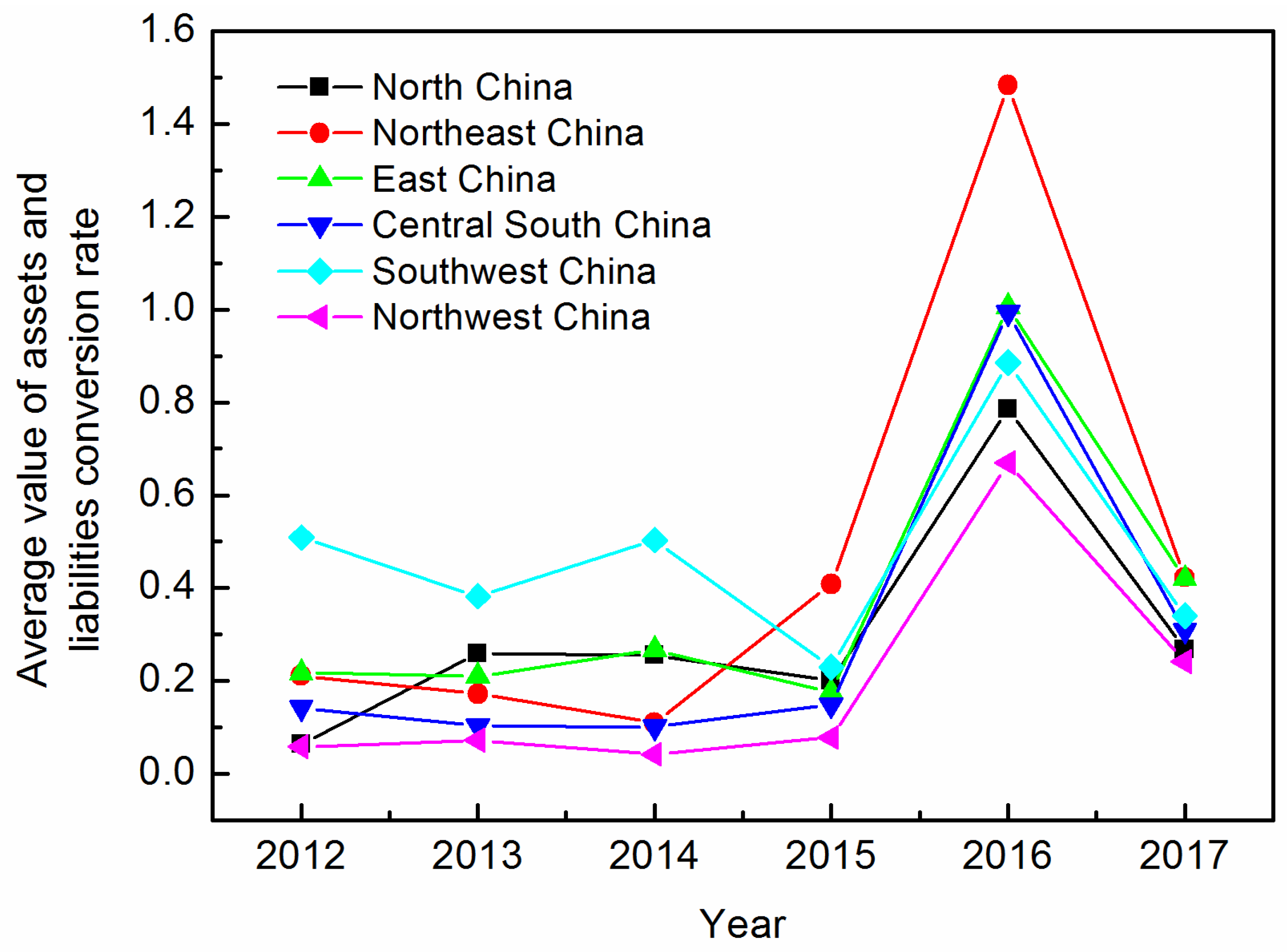
4.1. Calculation of Conversion Rates of Assets and Environmental Liabilities

Based on the panel data of 31 provinces in China from 2012 to 2017, this study used the Super-SBM model with undesirable outputs to measure the conversion efficiency between economic assets, resource assets, and environmental liabilities of China’s provincial local governments, as shown in

Table 2. Conversion efficiency of economic and resource assets and environmental liabilities by province.

DMU	2012	2013	2014	2015	2016	2017	Average	Rank
Beijing	0.0249	0.0258	0.0284	0.0301	0.0627	0.0235	0.0326	29
Tianjin	0.0193	0.0249	0.0248	0.0496	1.1646	0.0497	0.2222	22
Hebei	0.1288	1.0493	1.0079	0.2027	0.7319	0.1340	0.5424	8
Shanxi	0.1095	0.1337	0.1614	0.6824	1.1338	1.0636	0.5474	7
Inner Mongolia	0.0349	0.0639	0.0536	0.0387	0.8382	0.0697	0.1832	24
Liaoning	0.5094	0.3425	0.2047	1.0678	1.4383	0.0301	0.5988	5
Jilin	0.0966	0.1014	0.0656	0.0736	1.9820	1.0592	0.5631	6
Heilongjiang	0.0283	0.0727	0.0597	0.0852	1.0304	0.1800	0.2427	19
Shanghai	0.4909	0.6587	1.1444	0.4386	1.8587	1.0857	0.9462	1
Jiangsu	0.1963	0.1681	0.1495	0.1870	0.6566	0.0224	0.2300	20
Zhejiang	0.3275	0.2314	0.2086	0.2643	1.5961	0.3602	0.4980	9
Anhui	0.0702	0.0842	0.0562	0.0626	0.5967	0.0042	0.1457	27
Fujian	0.1971	0.1676	0.0960	0.1742	0.9426	1.0789	0.4427	10
Jiangxi	0.1381	0.0565	0.1259	0.0488	1.0709	0.3590	0.2999	16
Shandong	0.1049	0.1051	0.0867	0.0550	0.3197	0.0293	0.1168	28
Henan	0.1256	0.0789	0.0978	0.0722	0.6594	0.0671	0.1835	23
Hubei	0.1548	0.1584	0.1326	0.2603	1.0569	0.0071	0.2950	17
Hunan	0.2236	0.0379	0.1040	0.1378	1.0529	0.1673	0.2872	18
Guangdong	0.2245	0.1952	0.1705	0.1457	1.0001	0.0836	0.3033	15
Guangxi	0.0563	0.0738	0.0740	0.2321	1.0005	0.4811	0.3196	14
Hainan	0.0675	0.0779	0.0268	0.0430	1.1883	1.0466	0.4083	11
Chongqing	0.2260	0.2073	0.1445	0.1681	1.2488	0.0896	0.3474	13
Sichuan	1.0020	0.4470	1.0091	0.2486	1.0799	0.0151	0.6336	4
Guizhou	1.1708	0.2522	1.0506	0.2519	1.0457	0.3401	0.6852	3
Yunnan	0.1339	1.0037	0.3096	0.4203	1.0496	1.2370	0.6923	2
Xizang	0.0111	0.0023	0.0032	0.0605	0.0035	0.0168	0.0162	31
Shanxi	0.1117	0.0917	0.0811	0.0822	0.5190	0.0528	0.1564	26
Gansu	0.0573	0.0583	0.0436	0.0413	1.0152	0.1375	0.2255	21
Qinghai	0.0184	0.0141	0.0081	0.0094	0.0055	0.0631	0.0198	30
Ningxia	0.0650	0.1559	0.0626	0.1992	1.2223	0.6030	0.3847	12
Xinjiang	0.0384	0.0393	0.0137	0.0580	0.5891	0.3534	0.1820	25
Average	0.1988	0.1994	0.2195	0.1900	0.9406	0.3326

.

On the whole, during 2012–2017, the average conversion efficiency of the assets and environmental liabilities of the 31 provinces was 0.1988, 0.1994, 0.2195, 0.1900, 0.9406, and 0.3326 each year, respectively. Shanghai, Yunnan, Sichuan, and Guizhou had the greatest efficiency, followed by Liaoning, Jilin, Shanxi, Hebei, Zhejiang, Fujian, and Hainan, where the average conversion efficiency was greater than 0.4; the average in other provinces was less than 0.4. Over time, except for Yunnan and Fujian Province, the conversion efficiency generally increased first and then decreased, with 2016 as an inflection point of the change. Compared with 2012–2015, the number of provinces and cities that were found to be efficient increased significantly in 2016; those not found to be efficient increased in 2014 and increased slightly in 2017 after decreasing in 2015. The conversion efficiency of a few provinces improved from non-efficient to efficient; for example, the conversion efficiency of Shanxi Province increased from 0.109488 in 2012 to 0.68237220 in 2015 and increased again to 1.06355 in 2017. It is worth noting that for three consecutive years, from 2015 to 2017, the conversion efficiencies in Shanghai, Shanxi, and Yunnan were greater than 0.4, and in 2016 and 2017, they were greater than 1.

It can be seen from Table 2 that there were regional differences in conversion efficiencies between local government assets and environmental liabilities. Overall, the conversion efficiencies of assets and environmental liabilities in Southwest and North China were relatively close, with an average over five years of about 0.68. However, the conversion efficiencies in Xinjiang, Xizang, Inner Mongolia, Beijing, and Tianjin were significantly lower at 0.4. The conversion efficiencies of economic and resource assets and environmental liabilities of local governments in China showed significant differences across regions and had obvious regional characteristics.

According to the administrative regions, China’s provinces are divided into six regions: North China (including Beijing, Tianjin, Hebei, Shanxi, and Inner Mongolia), Northeast China (including Liaoning, Jilin, and Heilongjiang), East China (including Shandong, Jiangsu, Anhui, Zhejiang, Jiangxi, Fujian, and Shanghai), Central South China (including Henan, Hubei, Hunan, Guangdong, Guangxi, and Hainan), Southwest China (including Sichuan, Chongqing, Yunnan, Guizhou, and Xizang), and Northwest China (including Shanxi, Gansu, Qinghai, Ningxia, and Xinjiang). The average asset and environmental liability conversion rates of each region from 2012 to 2017 are shown in Figure 1.

Among the top 10 provinces in 2016–2017, most were in Southwest and North China, and only Shanghai, Zhejiang, and Fujian Provinces, with the highest level of economic development, were in the top 10. The main reason for this may have been the differences in regional development and the uneven distribution of resources in different regions. As can be seen from Figure 1, the trends of asset conversion rates in the regions from 2015 to 2017 were similar. From 2012 to 2013, only North and Northwest China showed upward trends. From 2013 to 2014, the regions generally decreased, except for East and Southwest China. From 2014 to 2015, Northeast, Northwest, and Central South China showed upward trends, while other regions showed downward trends.

When we explored the reasons, on the one hand, the echelon differences in the degree of industrialization in the eastern, central, and western provinces determined the stock differences in pollution emissions, which inevitably affected the conversion efficiencies of the economic and resource assets and environmental liabilities when the funds for local environmental protection were relatively scarce. On the other hand, almost all the provinces that focused on the development of western provinces and the rise of central provinces were considered effective. What they had in common was that, compared with the eastern region, the total economic volume was not very large, but the resource assets were relatively rich. Although the central and western regions were economically underdeveloped with a low economic aggregate, the state attached great importance to pollution control in these regions while implementing the China’s Western Development Strategy. The pressure to provide environmental protection funds was relatively low. In addition, the central and western regions were rich in resource assets, which could provide more ecological benefits for environmental governance.

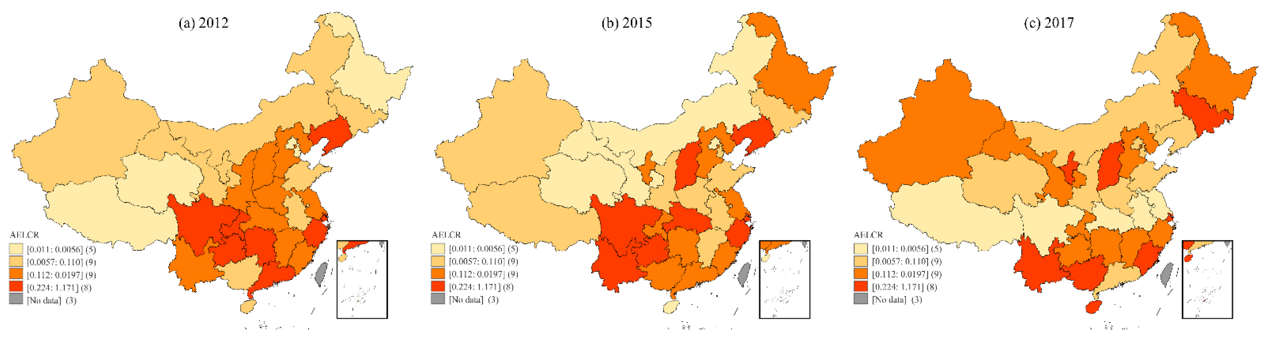
4.2. Analysis of the Spatial Evolution Characteristics of the Conversion Rates of Assets and Environmental Liabilities

In the test of the spatial autocorrelation effect, Moran’s I was used to test the spatial correlations or differences of the whole study area, while local spatial autocorrelation (LISA) was used to reflect the correlation degrees between certain geographical phenomena or attribute values in adjacent geographical units.

The spatial measurement analysis needs a certain connection between spatial units; therefore, Hong Kong, Macao, Taiwan, and Hainan Province were not included in the research sample because of the difficulty of data acquisition and their geographical locations. The data were from the China Statistical Yearbook and Wind Database. Since there is a common boundary between adjacent provinces and municipalities, the K-nearest neighbor spatial weights matrix was selected, and the weight between each geographical unit and adjacent provinces is the reciprocal of their geometric distance, that is, the nearest neighbor spatial weights matrix, $\frac{1}{d_{ij}}$.

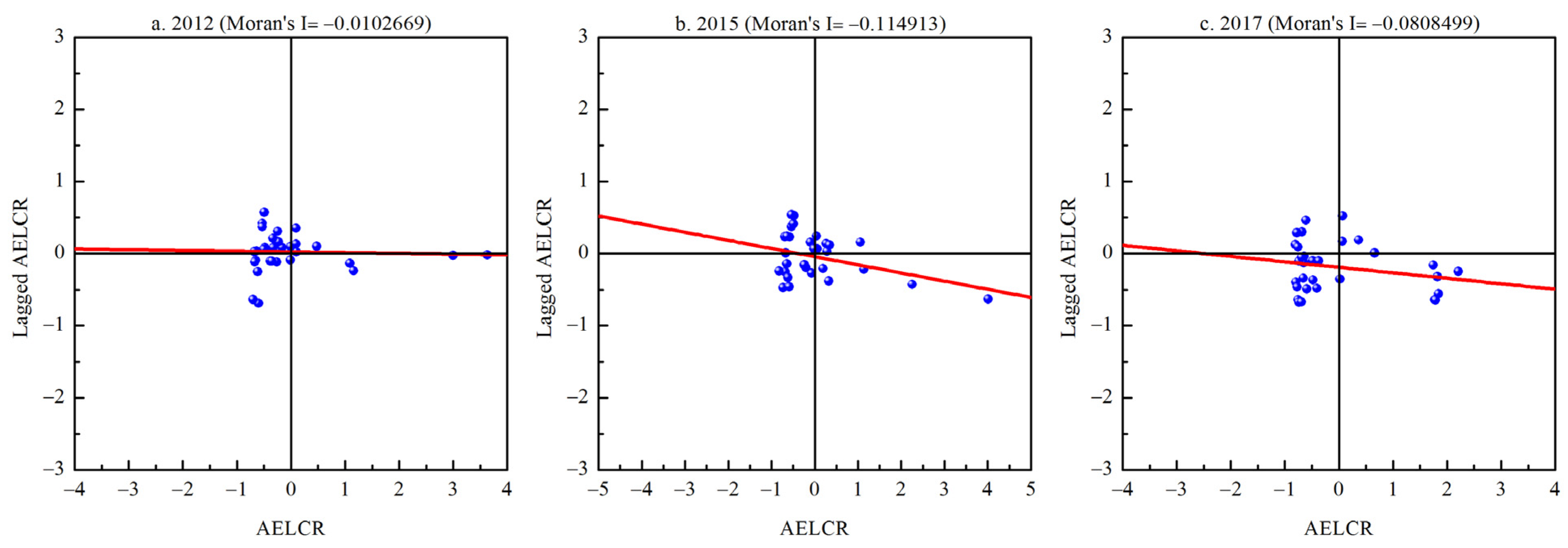
4.2.1. Analysis of Global Spatial Autocorrelations

This study used the P index to explore the spatial correlations. Based on the statistical analysis of the conversion rates of assets and environmental liabilities of each province in 2012, 2015, and 2017, a spatial quartile distribution map was created. The darker the color, the higher the assets and environmental liabilities conversion rate (AELCR) of the province, as shown in Figure 2.

Looking at Figure 2a–c, regarding 2012, the brownish-red areas include Sichuan, Chongqing, Guizhou, Hunan, Guangdong, Zhejiang, Liaoning, and Shanghai; orange areas include Yunnan, Fujian, Jiangxi, Hubei, Jiangsu, Henan, Shaanxi, Shanxi, and Hebei; light orange areas include Xinjiang, Gansu, Inner Mongolia, Ningxia, Shandong, Anhui, Jilin, and Guangxi; and Xizang, Heilongjiang, Qinghai, Beijing, and Tianjin are white.

Regarding 2015, the brownish-red areas include Liaoning, Shanxi, Sichuan, Hubei, Zhejiang, Shanghai, Guizhou, and Yunnan; orange areas include Ningxia, Heilongjiang, Hebei, Jiangsu, Chongqing, Hunan, Guangxi, Guangdong, and Fujian; light orange areas include Xinjiang, Xizang, Shaanxi, Henan, Shandong, Anhui, Jiangxi, Jilin, Tianjin, and Inner Mongolia; and white areas include Gansu, Qinghai, Anhui, and Beijing. From 2012 to 2015, the assets and environmental liabilities conversion rates of Chongqing, Hunan, Guangdong, Inner Mongolia, Fujian, Jiangxi, Henan, and Shaanxi decreased, while those of Yunnan, Hubei, Shanxi, Xizang, Ningxia, Heilongjiang, and Tianjin increased.

Regarding 2017, the brownish-red areas include Ningxia, Yunnan, Guangxi, Fujian, Shanxi, Shanghai, and Jilin; the orange areas include Xinjiang, Gansu, Heilongjiang, Hebei, Chongqing, Guizhou, Hunan, Jiangxi, and Zhejiang; the light orange areas include Inner Mongolia, Qinghai, Shaanxi, Henan, Shandong, Guangdong, Liaoning, Beijing, and Tianjin; and the white areas include Xizang, Sichuan, Hubei, Anhui, and Jiangsu. From 2015 to 2017, the conversion rates of Ningxia, Guangxi, Fujian, Jilin, Xinjiang, Gansu, Jiangxi, Inner Mongolia, Qinghai, and Beijing increased, while those of Jiangsu, Guizhou, Zhejiang, Guangdong, Liaoning, Sichuan, Hubei, Anhui, and Jiangsu decreased; among them, Sichuan and Hubei decreased by a large margin, while Shanghai showed a relatively low level in those three years.

The global spatial autocorrelation test was carried out using GeoDa software, and Moran’s I scatter charts of the AELCR of each province in 2012, 2015, and 2017 were drawn. In Figure 3, the horizontal axis is AELCR, and the vertical axis is lagged AELCR, which is the weighted average value of adjacent values. As shown in the figure, Moran’s I values of China’s provincial AELCRs in 2012, 2015, and 2017 were all negative at −0.0102669, −0.114913, and −0.0808499, respectively, indicating that the conversion rate had negative spatial correlations and heterogeneity.

Table 3. Spatial correlation pattern division and meaning of Moran’s I scatter diagram.

Quadrant	Aggregate Type	Meaning	Spatial Correlation
First quadrant	(H,H)	Area with a high assets and environmental liabilities conversion rate surrounded by areas with high conversion rates	Positive correlation
Second quadrant	(L,H)	Area with a low assets and environmental liabilities conversion rate surrounded by areas with high conversion rates	Negative correlation
Third quadrant	(L,L)	Area with a low assets and environmental liabilities conversion rate surrounded by areas with low conversion rates	Negative correlation
Fourth quadrant	(H,L)	Area with a high assets and environmental liabilities conversion rate surrounded by areas with low conversion rates	Positive correlation

shows the spatial correlation pattern division and meaning of the Moran’s I scatter diagram.

The spatial correlation in the first and third quadrants is positive, which indicates dependence between similar geographical observation units. The spatial correlation in the second and fourth quadrants is negative, which indicates heterogeneity between geographical observation units.

As shown in Figure 3, most provinces in 2012 and 2015 were in the second and third quadrants, which shows that in those years, the AELCRs of China’s provinces mainly showed (L,H) and (L,L) agglomerations, that is, in areas with a low asset and environmental liability conversion rate, there were areas with a high conversion rate and areas with a low conversion rate. However, in 2017, the AELCRs of most provinces were in the second and fourth quadrants, and a few regions were in the first and third quadrants, which indicates that the asset–liability conversion rate of each province gradually showed the characteristics of (L,H) and (H,L) agglomerations, and the evolution process more clearly reflected the heterogeneity of the conversion rate of different provinces. It can be concluded that the AELCRs among different regions in China had the characteristics of spatial agglomeration and heterogeneity, gradually changing to heterogeneity.

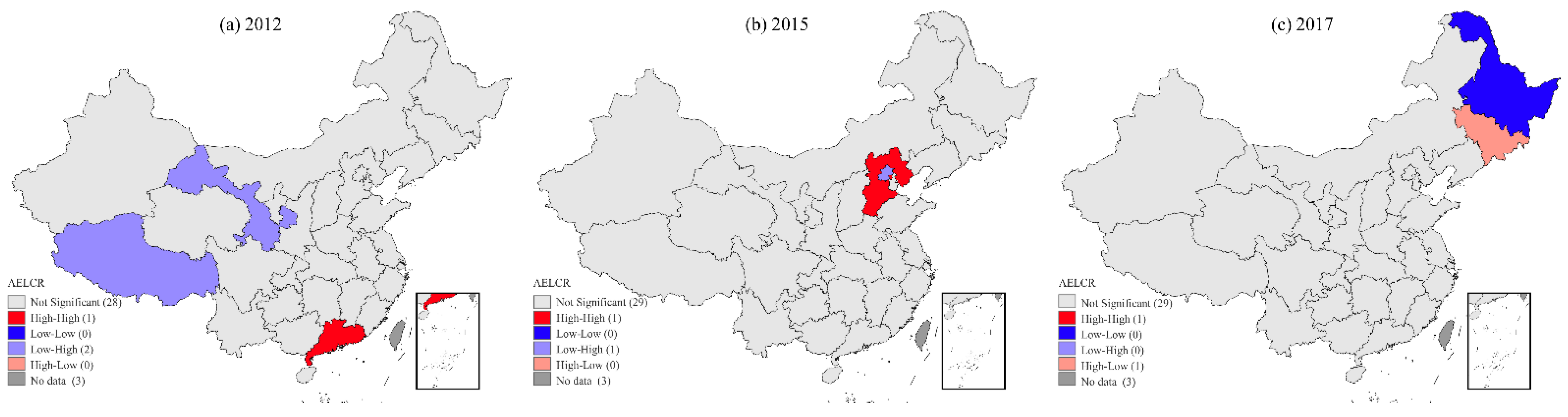
4.2.2. Analysis of Local Spatial Autocorrelations

Based on the LISA cluster analysis of the asset and environmental liability conversion rates in 2012, 2015, and 2017, the spatial dependence and heterogeneity can be observed directly from the aggregation or dispersion of different colors in the local spatial effect map.

Figure 4 shows the LISA spatial clustering distribution maps with the local spatial clustering characteristics of each province. Figure 5 shows the p-value of the significance level of the LISA index. The green part of the figure shows the area of the local spatial clustering feature that passed the 5% significance test. The features were more obvious in this area.

As can be seen from Figure 4, the spatial clustering distribution of the conversion rates changed significantly between 2012, 2015, and 2017. In 2012, Guangdong Province showed (H,H) clustering (red), while Gansu and Xizang showed (L,H) clustering (blue-purple), indicating that the conversion rate in 2012 was low for Gansu and Xizang but was high for their surrounding provinces, and the three regions were significant at a level of 0.05.

In 2015, Hebei showed (H,H) clustering (red), and Beijing and Tianjin showed (L,H) clustering (blue-purple), indicating that the conversion rates for the two regions were low, but those of the surrounding regions were high. Hebei Province was significant at the level of 0.01, while Beijing and Tianjin were significant at the level of 0.5.

In 2017, Heilongjiang showed (L,L) clustering (blue), and Jilin showed (H,L) clustering (pink), and the three regions were significant at the 0.05 level. Most of the regions in the figure are gray, which shows that the conversion rates in most regions of China did not have a significant local correlation with neighboring regions. This indicates that the provinces had not yet formed linked environmental governance; therefore, it is still necessary to enhance the linkage mechanism to promote environmentally friendly and coordinated development.

5. Analysis of Factors Influencing the Spatial Evolution of the Conversion Rates of Assets and Environmental Liabilities

5.1. Index Selection and Data Preprocessing

This study selected data from 2012 to 2017 for 31 provinces in China to examine the asset and environmental liability conversion rate (AELCR), urban population proportion (URB), resource tax (TY), urban environmental infrastructure construction investment (INE), per capita GDP, and provincial R&D investment factors, and obtained a total of 1260 samples. Hong Kong, Macao, Taiwan, and Hainan were not included in the empirical study due to their geographical location. The data were from the China Statistical Yearbook and Wind Database.

Urbanization has an important impact on urban meteorology, which can change the atmospheric diffusion capacity of urban areas, thus affecting the concentration of pollutants [51]. The impact of urbanization on the efficiency of environmental remediation mainly comes from the increased population, because when the population increases, the “three wastes” and other pollutants from urban production and life will increase, which is likely to aggravate urban pollution. Therefore, this study used the proportion of non-agricultural population in the total population to express the urbanization level [52].

In view of the negative externality of pollution, resource tax has gradually become an important means to control environmental pollution, which can obtain the double dividend of environmental protection and economic growth. Urban infrastructure is a public service system that is used to ensure the normal social and economic activities of a country or region. Its social benefits are far greater than its economic benefits and are of great significance to social development [53]. Constructing an environmental infrastructure will affect urban environmental governance, and improving the environmental infrastructure will help to form a positive environmental governance cycle. Therefore, this study selected the amount of investment amount of urban environmental infrastructure construction to represent the level of urban environmental infrastructure construction.

At the same time, according to the theory of the environmental Kuznets curve, per capita income is related to environmental quality. After studying the relationship between environmental quality and per capita income, Grossman et al. and Panayotou [54,55] pointed out that pollution increased with increased per capita GDP in low-income areas and decreased in high-income areas. Therefore, this study selected the per capita GDP of all provinces in China to represent the economic development level of this region. The technology effect is introduced into the expanded research of the environmental Kuznets curve, and progress in innovation technology is conducive to environmental improvement [56,57,58]. Therefore, this study selected R&D investment to represent the technical level of each province, and the detail indexes are shown in

Table 4. Variable definitions.

Variable	Index	Description
Regional economic development	AGDP	Per capita GDP
Urban environment infrastructure	INE	Urban environmental infrastructure construction investment
Provincial technological innovation	ARD	Provincial R&D investment
Urbanization	URB	Urban population proportion
Resource tax	TY	Resource tax amount

.

5.2. Spatial Econometric Modeling and Analysis of Panel Data

5.2.1. Spatial Lag Model (SLM)

In the spatial lag model (SLM), the spatial correlation of explanatory variables was represented using the spatial lag term of the explained variables, where the following model is established:

$$\begin{array}{l}LnAELCR={\gamma }_{1}LnURB+{\gamma }_{2}LnTY+{\gamma }_{3}LnINE+{\gamma }_{4}LnAGDP+{\gamma }_{5}LnARD\\ +\rho WLnV+{\epsilon }_1\end{array}$$

(16)

In this model, WLnV represents the explained variable of spatial lag, ρ represents the spatial autoregressive coefficient, and its estimated value and positive and negative values indicate the size and direction (positive or negative) of the geospatial correlation, respectively. W is the n-dimensional spatial weight matrix, which is generated by using the proximity relation. The set matrix was imported into the .shp file of the map with GeoDa software.

In this study, maximum likelihood (ML) estimation was used for regression analysis of the SLM model with a spatial lag term, and the estimation result was obtained using MATLAB software. From the results, the per capita GDP coefficient was 0.002469 and p = 0.8796, which did not pass the significance level test of p = 0.1, indicating that the index had little impact on the provincial asset and environmental liability conversion rates; therefore, the per capita GDP index was excluded. After sorting out the indicators,

Table 5. ML estimation results of factors affecting the conversion rates of assets and environmental liabilities (AELCRs) in the SLM model.

Variable	Regression Coefficient	p-Value
ρ	0.167968	0.000000 ***
LnURB	1.003195	0.000000 ***
LnTY	−1.177954	0.092769 *
LnINE	−0.057654	0.035989 **
LnAGDP	0.002469	0.8796
LnARD	0.016775	0.086342 *
R2	0.8993
LogL	164.36316
LM-Test	50.5341	0.000 ***
Robust LM-Test	10.7978	0.001 ***

Note: p is significance at *** p < 0.01, ** p < 0.05, * p < 0.1.

was obtained.

5.2.2. Spatial Error Model (SEM)

When the spatial correlation is explained by other variables that are not estimated by the explanatory variables, it can be determined that the spatial error is the cause of the spatial correlation. As such, the spatial error model (SEM) was used to measure the spatial correlation. The set model was as follows:

$$\begin{array}{l}LnAELCR={\alpha }_{1}LnURB+{\alpha }_{2}LnTY+{\alpha }_{3}LnINE+{\alpha }_{4}LnAGDP+{\alpha }_{5}LnARD\\ +\lambda LnW\times \mu +{\epsilon }_2\end{array}$$

(17)

In this model, λ is the autocorrelation coefficient of spatial error, which represents the spatial correlation degree between regression residuals, and LnW×μ represents the spatial lag error term. Maximum likelihood (ML) was used to regress the SEM model considering the spatial lag term, and the ML estimation results were obtained by using MATLAB software, as shown in

Table 6. ML estimation results of factors affecting conversion rates of assets and environmental liabilities (AELCRs) in the SEM model.

Variable	Regression Coefficient	p-Value
λ	0.552995	0.000000 ***
LnURB	1.002554	0.000000 ***
LnTY	−1.239060	0.111760
LnINE	0.033583	0.268458
LnAGDP	0.005421	0.7538
LnARD	0.004629	0.625861
R2	0.8764
LogL	178.67727
LM-Test	123.4819	0.000 ***
Robust LM-Test	83.7456	0.000 ***

Note: p is significance at *** p < 0.01.

.

5.2.3. Analysis of SLM and SEM Model Results

To explore the factors that influenced the asset and environmental liability conversion rates, a spatial econometric model and MATLAB were used to estimate the SLM and SEM models, and then the results of the two models were compared.

According to the estimation results given in Table 5 and Table 6, the goodness of fit R² values of the SLM and SEM were 0.8993 and 0.8764, respectively. The results show that the SLM and SEM had better fits, and the SLM was slightly better. After considering the spatial effect, the model using maximum likelihood estimation can effectively avoid the result bias of the traditional least square estimation method. As can be seen from Table 5, the log-likelihood value of the SLM was 164.36316, the LM value was 50.5341, and the p-value was 0.000, which was less than 0.01, passing the significance test of the 99% confidence interval. The value of the robust LM was 10.7978, and the p-value was 0.001, which also passed the 99% significance test, indicating that both were very significant. The log-likelihood value of the SEM was 178.67727, which was greater than that of the SLM model. The LM value was 123.4819, and its p-value was 0.000; it passed the 99% significance test. The robust LM value was 83.7456, and its p-value was 0.000, which also passed the 99% significance test.

Comparing the SLM and SEM, it can be seen from the regression results that the SLM had a better goodness of fit, but the LM value, robust LM value, and the corresponding parameters of the two models were better; therefore, the SLM was better than the SEM. The SLM should be chosen to study the factors that influence the spatial evolution of the asset and environmental liability conversion rate in China.

The spatial lag model was determined to be the following:

$$\begin{array}{l}LnAELCR=1.003195LnURB+1.177954LnTY+0.057654LnINE\\ +0.016775LnARD+0.167968WLnV+{\epsilon }_1\end{array}$$

(18)

The p-values of the spatial autoregressive coefficient and LnURB coefficient passed the 99% confidence interval test, the p-value of the LnINE coefficient passed the 95% confidence interval test, and the p-values of the coefficients corresponding to LnTY and LnRD passed the 90% confidence interval test, but the coefficient of LnAGDP did not pass the significance test; therefore, the per capita GDP index was eliminated.

The urbanization rate (URB) and provincial R&D investment were positively correlated with the asset and environmental liability conversion rate, which shows that these two indicators had a positive effect on the conversion rate, and the coefficient of urbanization rate was relatively large at a significance level of 0.01, which shows that it had a significant driving effect on the conversion rate, verifying hypotheses H1c and H1d. The coefficients of resource tax revenue and urban environmental infrastructure construction investment were negative, which indicates that the two indicators had a negative effect on the conversion rate, where the former was larger, which indicates that the index had a more obvious negative impact on the conversion rate of assets and environmental liabilities; therefore, hypothesis H1e was verified, but H1a and H1b were not.

6. Conclusions and Implications

6.1. Conclusions

Focusing on the indexes of the asset and environmental liability conversion rate, this study first used the Super-SBM model with undesirable outputs to measure its efficiency value and then used GeoDa software to analyze its spatial characteristics. Finally, the spatial econometric model was used to explore the influencing factors, where the model was estimated with MATLAB.

The results demonstrate that China’s provincial economy had the characteristics of unbalanced development and large gaps in development levels. At the same time, there were significant differences in the efficiencies of environmental protection fiscal expenditures between regions. From the local point of view, most provinces had not formed a significant spatial correlation; at the same time, from 2012 to 2017, local similarities in the national asset and environmental liability conversion rates decreased, and heterogeneity gradually increased.

Our findings also indicate that promoting urbanization and provincial R&D investment was conducive to improving the asset and environmental liability conversion rate, but resource tax and urban environmental infrastructure investment were negatively correlated with the conversion rate. With the advancement of urbanization processes and the development of industry, the traditional processes were replaced by the tertiary industry (that is service sector), with its low pollution and low energy consumption, which improved the environmental quality and the efficiency of government fiscal expenditure on environmental protection. Urbanization improves labor productivity, changes the economic structure of the region, alleviates the growth trend of industrial pollution emissions, and helps to improve the efficiency of government expenditure [33,34]. The higher the provincial R&D investment, the higher the level of innovation and technology of the associated cities, which reduces traditional high-energy-consumption technology use, reduces environmental pollution, and improves the reuse efficiency of pollutants [30], which are also conducive to improving the efficiency of government fiscal expenditure on environmental protection. Regions with higher resource taxes are more likely to bear higher environmental liabilities, and at the same time, such taxes could increase the economic cost of enterprises and lessen the enthusiasm for environmental protection [35], which will hinder the improvement of the conversion rate of assets and environmental liabilities to a certain extent. There are two possible explanations for the negative correlation between the investment in urban environmental infrastructure and the conversion rate of assets and environmental liabilities for a given region: on the one hand, the higher the investment in infrastructure, the more likely it is to show that the current environmental liabilities are higher and the environmental base is poorer; on the other hand, higher investment in infrastructure shows that the current environmental infrastructure is under construction and has not yet shown its environmental governance effect.

6.2. Managerial and Policy Implications

Under the premise of limited financial funds for environmental protection, the government should deeply integrate the concept of performance into the process of using financial funds for environmental governance and protection in various regions, improve the performance management mechanism of such financial expenditure, optimize the level of environmental performance in various regions, pay attention to balancing economic development and environmental protection, and seek sustainable and efficient economic development based on environmental friendliness.

The central and western regions are rich in natural resources, which can provide more ecological benefits for environmental governance. Affected by western regional development and central prosperity policies, these regions should improve the efficiency of environmental governance by increasing the protection of natural resources rather than blindly investing in environmental protection. For the eastern region, with its relatively high economic prosperity but fewer natural resources, the government should increase the funds for environmental protection and address the environmental liabilities by increasing pollution control. The results indicate that the provinces in China still have not formed linked environmental governance, and the conversion rate of assets and environmental liabilities shows more regional heterogeneity. It is necessary to strengthen the linkage mechanisms of environmental governance between the provinces, promote the coordinated development of environmentally friendly policies, and make strong use of the positive environmental spillover effect.

7. Limitations and Outlook

In this study, the Super-SBM model with undesirable outputs was used to measure the assets and environmental liabilities conversion rates (AELCRs) of China’s provinces, and the spatial measurement model was used to explore its spatial evolution characteristics and influencing factors, which expanded the methodology used to evaluate the efficiency of the government’s fiscal expenditure for environmental protection. Different from the traditional method of using the Malmquist index to explore dynamic changes in the conversion rate, this study analyzed the transformation rate from the perspective of geographical space. However, there were some limitations:

(1) Given the difficulty regarding data acquisition, this study made some trade-offs in the selection of input and output indicators for measuring the AELCRs. In the future, the number of indexes of economic and resource assets can be increased to enhance their representativeness as much as possible.

(2) The data sample was limited. Due to the incompleteness of the statistical yearbook and other reasons, only six years’ worth of data was used; therefore, long-term data should be added for a more complete view of the dynamic changes. The desirable output indicators can be described in more detail, and the air pollutants can be subdivided into common international statistical diameters, such as PM10 and PM2.5. The research results would be more comparable if international monitoring indicators were used.

(3) The influencing factors could have been more comprehensive. From the empirical results of this study, we can see that the goodness of fit of the two models did not reach 0.90, indicating that some significant factors may not have been included in the empirical study, such as education; therefore, the explanation of some models still needs to be improved. For example, the air-quality improvement index can show increased smoke and dust pollutants, and at the same time, the research can be expanded to distinguish and explore the reactions of the asset and environmental liability conversion rate to different factors.

References

1. Abraham, K.S. Environmental liability and the limits of insurance. Colum. L. Rev. 1988, 88, 942–988. [Google Scholar] [CrossRef] [Green Version]
2. Rauscher, M. Economic Growth and Tax-competition Leviathans. Int. Tax Public Finan. 2005, 12, 457–474. [Google Scholar] [CrossRef] [Green Version]
3. Wang, H. Review on the development of resource assets appraisal. China Manag. Inf. 2012, 15, 14–16. [Google Scholar]
4. Beltrán-Esteve, M.; Gómez-Limón, J.A.; Picazo-Tadeo, A.J.; Reig-Martínez, E. A metafrontier directional distance function approach to assessing eco-efficiency. J. Prod. Anal. 2014, 41, 69–83. [Google Scholar] [CrossRef]
5. Färe, R.; Grosskopf, S.; Lovell, C.A.K.; Pasurka, C. Multilateral productivity comparisons when some outputs are undesirable: A nonparametric approach. Rev. Econ. Stat. 1989, 71, 90–98. [Google Scholar] [CrossRef]
6. Chung, Y.H.; Färe, R.; Grosskopf, S. Productivity and undesirable outputs: A directional distance function approach. Environ. Manag. 1997, 51, 229–240. [Google Scholar] [CrossRef] [Green Version]
7. Wang, Y.; Wen, Z.; Cao, X.; Zheng, Z.; Xu, J. Environmental efficiency evaluation of China’s iron and steel industry: A process-level data envelopment analysis. Sci. Total Environ. 2020, 707, 135903. [Google Scholar] [CrossRef]
8. Chen, L.M.; Wang, W.P.; Wang, B. Economic efficiency, environmental efficiency and ecological efficiency of “two horizontal and three vertical” urbanized areas—An Empirical Analysis Based on mixed directional distance function and composite graph method. Chin. Soft. Sci. 2015, 2, 96–109. [Google Scholar]
9. Zhu, H.; Fu, Q.; Wei, Q. Empirical Study on efficiency accounting and influencing factors of local government’s environmental protection expenditure. Chin. J. Popul. Resour. Environ. 2014, 24, 91–96. [Google Scholar]
10. Yin, K.; Wang, S.R.; Yao, L.; Liang, J. Ecological efficiency evaluation of environmental protection model cities in China. Acta Ecol. Sin. 2011, 31, 5588–5598. [Google Scholar]
11. Huang, Y.P.; Shi, Q.P. Research on regional environmental efficiency and environmental total factors in China—Based on SBM model with R & D input. China Popul. Resour. Environ. 2015, 25, 25–34. [Google Scholar]
12. Becerra-Ornelas, A.U.; Nuñez, H.M. The technical efficiency of local economies in Mexico: A failure of decentralized public spending. Ann. Reg. Sci. 2019, 62, 247–264. [Google Scholar] [CrossRef]
13. Flick, W.A. Environmental repercussions and the economic structure: An input-output approach: A comment. Rev. Econ. Stat. 1974, 56, 107–109. [Google Scholar] [CrossRef]
14. De Borger, B.; Kerstens, K.; Moesen, W.; Vanneste, J. Explaining differences in productive efficiency: An application to Belgian municipalities. Public Choice 1994, 80, 339–358. [Google Scholar] [CrossRef]
15. Li, J.; Li, X.M.; Liu, Z.Q. Evaluation and analysis of urban ecological environment based on urbanization development system. China Popul. Resour. Environ. 2009, 19, 156–161. [Google Scholar]
16. Liu, B.X.; Wang, B.S.; Xue, G. Efficiency evaluation of local government environmental pollution control in China—Based on three-stage bootstrapped DEA method. J. Zhongnan Univ. Econ. Law 2016, 1, 89–95, 160. [Google Scholar]
17. Zeng, X.G. Regional environmental efficiency and its influencing factors in China. Econ. Theor. Bus. Manag. 2011, 10, 103–110. [Google Scholar]
18. Chen, M. Does fiscal decentralization increase the efficiency of government environmental governance—Evidence from 31 provinces in China. Contemp. Econ. Manag. 2014, 36, 66–71. [Google Scholar]
19. Luo, L.Q.; Guo, X.L.A. study on the win-win balance between provincial environmental protection and economic development in China—Based on the perspective of environmental efficiency. Sci. Technol. Prog. Policy 2016, 33, 40–47. [Google Scholar]
20. Rong, J.B.; Yan, L.J.; Huang, S.R.; Zhang, G. Environmental efficiency assessment of Western China under carbon emission constraints. Chin. J. Appl. Ecol. 2015, 26, 1821–1830. [Google Scholar]
21. Yuan, H.; Xiu, F.D.; Zhu, C.N.; Jin, N.; Bai, L.Y. Spatial temporal pattern and influencing factors of industrial environmental efficiency in Jiangsu Province. Geogr. Geo-Inf. Sci. 2017, 33, 112–118. [Google Scholar]
22. Han, J.; Meng, D.A. Spatial effect of fiscal decentralization on ecological environment: Empirical data from provincial panel. Publ. Fin. Res. 2018, 3, 71–77. [Google Scholar]
23. Tone, K. A slacks-based measure of super-efficiency in data envelopment analysis. Eur. J. Oper. Res. 2002, 143, 32–41. [Google Scholar] [CrossRef] [Green Version]
24. Gao, J.; Qiao, G.M. Performance evaluation of environmental protection expenditure of provincial local governments Window-SBM three stages model based on pm2.5 bad output. J. Soochow Univ. 2019, 40, 103–111. [Google Scholar]
25. Zhang, Y.B.; Ma, C.; Jin, P.Z. The environmental regulation investment efficiency evaluation and its influencing factors analysis of china based on the SBM—TOBIT model of panel data. Econ. Manag. 2014, 36, 171–180. [Google Scholar]
26. Niu, T.; Zhao, S.G. An empirical study of the relationship between urban environmental infrastructure investment and economic growth. Urban Stud. 2010, 17, 128–131. [Google Scholar]
27. Sun, Y.; Wang, Y.K.; Yao, X.D. Study on environmental benefits evaluation of urban public infrastructure. China Popul. Resour. Environ. 2015, 25, 92–100. [Google Scholar]
28. He, X.G.; Wang, Z.L. Energy biased technology progress and green growth transformation: An empirical analysis based on 33 industries of China. China Ind. Econ. 2015, 32, 50–62. [Google Scholar]
29. Meng, W.S.; Zhang, Y. Natural resource endowment, path selection of technological progress, and green economic growth: An empirical research based on China’s provincial panel data. Resour. Sci. 2020, 42, 2314–2327. [Google Scholar]
30. Wang, P.; Xie, L.W. Pollution control investment, enterprise technical innovation and pollution control efficiency. China Popul. Resour. Environ. 2014, 24, 51–58. [Google Scholar]
31. York, R.; Rosa, E.A.; Dietz, T. STIRPAT, IPAT and IMPACT: Analytic Tools for Unpacking the Driving Forces of Environmental Impacts. Ecol. Econ. 2003, 46, 351–365. [Google Scholar] [CrossRef]
32. Ge, X.; Zhou, Z.; Zhou, Y.; Ye, X.; Liu, S. A Spatial Panel Data Analysis of Economic Growth, Urbanization and NOx Emissions in China. Int. J. Environ. Res. Public Health 2018, 15, 725. [Google Scholar] [CrossRef] [Green Version]
33. Chen, H.; Jia, B.; Lau, S.S.Y. Sustainable urban form for Chinese compact cities: Challenges of a rapid urbanized economy. Habitat Int. 2008, 32, 28–40. [Google Scholar] [CrossRef]
34. Liddle, B. Demographic dynamics and per capita environmental impact: Using panel regressions and household decompositions to examine population and transport. Popul. Environ. 2004, 26, 23–39. [Google Scholar] [CrossRef]
35. Chen, S.M.; He, L.Y. Environment, Health, and Economic Growth: Optimal Allocation of Energy Tax Revenue. Econ. Res. 2017, 52, 120–134. [Google Scholar]
36. Schwartz, J.; Repetto, R. Nonseparable Utility and the Double Dividend Debate: Reconsidering the Tax-Interaction Effect. Environ. Res. Econom. 2000, 15, 149–157. [Google Scholar] [CrossRef]
37. Pautrel, X. Pollution and life expectancy: How environmental policy can promote growth. Ecol. Econ. 2009, 68, 1040–1051. [Google Scholar] [CrossRef] [Green Version]
38. Marlin, J.T. Accounting for pollution. J. Account 1973, 2, 41–46. [Google Scholar]
39. Hoehn, J.P.; Randall, A. A satisfactory benefit cost indicator from contingent valuation. J. Environ. Econ. Manag. 1987, 14, 1226–1247. [Google Scholar] [CrossRef]
40. Freeman, A.M., III. The Measurement of Environmental and Resource Values: Theory and Methods; Resources for the Future Press: Washington, DC, USA, 2003. [Google Scholar]
41. Xu, J.L. On the problems of resource assets management. Macroeconomics 2005, 1, 34–37. [Google Scholar]
42. Beams, F.A.; Fertig, P.E. Pollution control through social cost conversion. J. Account. 1971, 132, 37–42. [Google Scholar]
43. Xu, L.; Liu, N.; Zhang, K. Study on the Efficiency of Converting Local Government Economics and Resource Assets to Environmental Liabilities under the Fiscal Restraint: An Empirical Analysis Based on Panel Data of the Sample of Chinese 29 Provinces from 2009 to 2013. Chin. Soft Sci. 2016, 30, 36–42. [Google Scholar]
44. Wan, J.X. Performance analysis of China’s budget expenditure on economic growth, resource consumption and environmental protection. Publ. Fin. Res. 2015, 3, 6–10. [Google Scholar]
45. Anselin, L. Spatial Econometrics: Methods and Models; Springer: Dordrecht, The Netherlands, 1988. [Google Scholar]
46. Getis, A.; Ord, J.K. The Analysis of Spatial Association by Use of Distance Statistics. Geog. Anal. 2010, 24, 127–145. [Google Scholar]
47. Anselin, L. Local indicators of spatial association—LISA. Geog. Anal. 1995, 27, 93–115. [Google Scholar] [CrossRef]
48. Mátyás, L.; Sevestre, P. (Eds.) The Econometrics of Panel Data: Fundamentals and Recent Developments in Theory and Practice; Advanced Studies in Theoretical and Applied Econometrics; Springer: Berlin/Heidelberg, Germany, 2008; Volume 46. [Google Scholar]
49. Huang, J.H.; Yang, X.G.; Hu, Y. Coordination degree and uncoordinated sources of resources, environment and economy—Based on CREE-EIE analysis framework. Chin. Ind. Econ. 2014, 7, 17–30. [Google Scholar]
50. Bai, X.J.; Wang, H.F.; Yan, W.K. Resource recession, science and education support and urban transformation—Research on the transformation efficiency of resource-based cities based on the bad output dynamic SBM model. Chin. Ind. Econ. 2014, 11, 30–43. [Google Scholar]
51. Liu, H.; Ma, W.; Qian, J.; Cai, J.; Ye, X.; Li, J.; Wang, X. Effect of urbanization on the urban meteorology and air pollution in Hangzhou. J. Meteorol. Res. 2015, 29, 950–965. [Google Scholar] [CrossRef]
52. Chen, S.M.; He, L.Y. Environment, health and economic growth: Optimal energy tax income distribution. Econ. Res. J. 2017, 52, 120–134. [Google Scholar]
53. Jiang, Y.; Zhu, X. Economic growth and infrastructure construction in China. Bus Rev. 2004, 9, 57–62, 64. [Google Scholar]
54. Grossman, G.M.; Krueger, A.B. Environmental Impacts of a North American Free Trade Agreement; National Bureau of Economic Research: Cambridge, MA, USA, 1991; Available online: https://www.nber.org/papers/w3914 (accessed on 28 August 2019).
55. Panayotou, T. Empirical Tests and Policy Analysis of Environmental Degradation at Different Stages of Economic Development; No. 992927783402676; International Labour Organization: Geneva, Switzerland, 1993. [Google Scholar]
56. Yin, J.; Zheng, M.; Chen, J. The effects of environmental regulation and technical progress on CO2 Kuznets curve: An evidence from China. Energy Policy 2015, 77, 97–108. [Google Scholar] [CrossRef]
57. Shao, L. Empirical Analysis on the Impact of Population, Economic Output, Economic Structure and Technological Progress on China’s SO_2 Emissions: Based on Extension of the Grossman Pollution Equation. Stat. Inf. Forum 2011, 26, 45–51. [Google Scholar]
58. Davis, I.S. Explaining changes in global sulfur emissions: An econometric decomposition approach. Ecol. Econ. 2002, 42, 201–220. [Google Scholar]
Figure 1. Line chart of average values of asset and liability conversion rates in China’s six regions, 2012–2017.
Sustainability 13 09164 g001
Figure 2. AELCR distributions in China’s provincial regions in 2012, 2015, and 2017.
Sustainability 13 09164 g002
Figure 3. Moran’s I scatter plots of AELCR in 2012, 2015, and 2017.
Sustainability 13 09164 g003
Figure 4. LISA clustering distribution of AELCRs in China’s provinces in 2012, 2015, and 2017.
Sustainability 13 09164 g004
Figure 5. Distribution of significant values of LISA indexes in China’s provinces in 2012, 2015, and 2017.
Sustainability 13 09164 g005